Dynamical Transitions in a Pollination
–
Herbivory Interaction: A Conflict between
Mutualism and Antagonism
Tomás A. Revilla1¤a
*, Francisco Encinas–Viso2¤b
1Centre for Biodiversity Theory and Modelling, Station d’Ecologie Expérimentale du Centre National de la Recherche ScientifiqueàMoulis, Moulis, France,2Community and Conservation Ecology Group, Centre for
Ecological and Evolutionary Studies, University of Groningen, Groningen, The Netherlands
¤a Current address: Biology Centre, Academy of Sciences of the Czech Republic,České Budějovice, Czech
Republic
¤b Current address: Centre for Australian National Biodiversity Research, Commonwealth Scientific and
Industrial Research Organisation, National Facilities and Collections, Canberra, Australia
Abstract
Plant-pollinator associations are often seen as purely mutualistic, while in reality they can be more complex. Indeed they may also display a diverse array of antagonistic interactions, such as competition and victim–exploiter interactions. In some cases mutualistic and antag-onistic interactions are carried-out by the same species but at different life-stages. As a con-sequence, population structure affects the balance of inter-specific associations, a topic that is receiving increased attention. In this paper, we developed a model that captures the basic features of the interaction between a flowering plant and an insect with a larval stage that feeds on the plant’s vegetative tissues (e.g. leaves) and an adult pollinator stage. Our model is able to display a rich set of dynamics, the most remarkable of which involves vic-tim–exploiter oscillations that allow plants to attain abundances above their carrying capaci-ties and the periodic alternation between states dominated by mutualism or antagonism. Our study indicates that changes in the insect’s life cycle can modify the balance between mutualism and antagonism, causing important qualitative changes in the interaction dynam-ics. These changes in the life cycle could be caused by a variety of external drivers, such as temperature, plant nutrients, pesticides and changes in the diet of adult pollinators.
Introduction
Il faut bien que je supporte deux ou trois chenilles si je veux connaître les papillons
Le Petit Prince, Chapitre IX–Antoine de Saint-Exupéry
Mutualism can be broadly defined as cooperation between different species [1]. In mutualistic interactions typically there are benefits and costs, in terms of resources, energy and time
a11111
OPEN ACCESS
Citation:Revilla TA, Encinas–Viso F (2015)
Dynamical Transitions in a Pollination–Herbivory Interaction: A Conflict between Mutualism and Antagonism. PLoS ONE 10(2): e0117964. doi:10.1371/journal.pone.0117964
Academic Editor:Jordi Garcia-Ojalvo, Universitat Pompeu Fabra, SPAIN
Received:October 14, 2014
Accepted:January 6, 2015
Published:February 20, 2015
Copyright:© 2015 Revilla, Encinas–Viso. This is an
open access article distributed under the terms of the
Creative Commons Attribution License, which permits unrestricted use, distribution, and reproduction in any medium, provided the original author and source are credited.
Data Availability Statement:All relevant data consists of graphs generated by computer scripts provided in the supplementary information file.
Funding:TAR was supported by the TULIP Laboratory of Excellence (ANR-10-LABX-41). FEV was supported by the OCE postdoctoral fellowship at CSIRO. The funders had no role in study design, data collection and analysis, decision to publish, or preparation of the manuscript.
devoted to them, but the net outcome is (+,+) in the final balance. However, there can be other kinds of costs, concerning detrimental interactions that run in parallel with mutualism, such as predation, parasitism or competition, involving the same parties. Moreover, some of these an-tagonistic interactions (e.g. competition) seem to be important for the evolution and stability of mutualism [2]. In general, these costs have important consequences at the population and community level because the net outcome of an interspecific association can turn out beneficial or detrimental and more interestingly, variable [3]. Variable interactions challenge the view that ecological communities are structured by well defined interactions at the species level such as competition (−,−), victim-exploiter (−,+) or mutualism (+,+).
Pollination is one of the most important mutualisms occurring between plants and animals. This form of trading resources for services greatly explains the evolutionary success of flower-ing plants in almost all terrestrial systems. It is responsible for the well beflower-ing of ecosystem ser-vices. During the larval stage of many insect pollinators, such as Lepidopterans (butterflies and moths), the larvae feed on plant leaves to mature and become adult pollinators [4–7]. These ontogenetic diet shifts [8] are very common and important in understanding the ecological and evolutionary dynamics of plant–animal mutualisms. Interestingly, in some cases larvae feed on the same plant species that they will pollinate as adults [6,9]. This shows that in several cases mutualistic and antagonistic interactions are exerted by the same species, and a potential conflict arises for the plant, between the benefits of mutualism and the costs of herbivory. One of the best known examples is the interaction between tobacco plants (Nicotiana attenuata) and the hawkmoth (Manduca sexta) [10,11], whose larva is commonly called the tobacco hornworm. There are other examples of this type of interaction in the genusManduca (Sphin-gidae), such as between the tomato plant (Lycopersicon esculentum) and the five-spotted hawk-moth (Manduca quinquemaculata) [12]. These larvae have received a lot of attention due to their negative effects on agricultural crops [13].
The interaction betweenManduca sextaandDatura wrightii(Solanacea) [6,14] is another good example illustrating the costs and benefits of pollination mutualisms [6].D. wrightii pro-vides high volumes of nectar and seems to depend heavily on the pollination service byM. sextaadults [14]. However,M. sextalarvae, which feed onD. wrightiivegetative tissue, can have severe negative effects on plant fitness [15,16]. We could assume that the benefits of polli-nation might outweigh the costs of herbivory for this mutualism to be relatively viable. The question is what are the conditions, in terms of benefits (pollination) and costs (herbivory), for this mutualistic interaction to be stable?
In the pollination–herbivory cases mentioned previously the benefits and costs for the plant are clearly differentiated. This is because the role of an insect as a pollinator or herbivore de-pends on the stage in its life cycle [17]. Thus, whether mutualism or herbivory dominates the interaction is dependent on insect abundance and its population structure. In other words the cost:benefitratio must be positively related with the insect’slarva:adultratio. For a hypothetical scenario in which the costs of herbivory (−) and the benefits of pollination (+) are balanced for
the plant (0), an increase in larval abundance relative to adults should bias the relationship to-wards a victim-exploiter one (−,+). Whereas an increase in adult abundance relative to larvae
should bias the relationship towards mutualism (+,+). Under equilibrium conditions, one would expect transitions (bifurcations) from (−,+) to (0,+) to (+,+) and vice-versa as relevant
parameters affecting the plant and the insect life-histories vary, such as flower production, mortalities or larvae maturation rates. However, under dynamic scenarios the outcome may be more complex: a victim–exploiter state (−,+) enhances larva development into pollinating
adults, but this tips the interaction into a mutualism (+,+), which in turn contributes greater production of larva leading back to a victim–exploiter state (−,+). This raises the possibility of
potentially lead to periodic alternation between mutualism and herbivory. Thus, when non-equilibrium dynamics are involved, questions concerning the overall nature (positive, neutral or negative) of mixed interactions may not have simple answers.
In this article we study the feedback between insect population structure, pollination and herbivory. We want to understand how the balance between costs (herbivory) and benefits (pollination) affects the interaction between plants (e.g.D. wrightii) and herbivore–pollinator insects (e.g.M. sexta)? Also what role does insect development have in this balance and on the resulting dynamics? We use a mathematical model which considers two different resources provided by the same plant species, nectar and vegetative tissues. Nectar consumption benefits the plant in the form of fertilized ovules, and consumption of vegetative tissues by larvae causes a cost. Our model predicts that the balance between mutualism and antagonism, and the long term stability of the plant–insect association, can be greatly affected by changes in larval devel-opment rates, as well as by changes in the diet of adult pollinators.
Methods
Our model concerns the dynamics of the interaction between a plant and an insect. The insect life cycle comprises an adult phase that pollinates the flowers and a larval phase that feed on non-reproductive tissues of the same plant. Adults oviposit on the same species that they polli-nate (e.g.D. wrightii–M. sextainteraction). Let denote the biomass densities of the plant, the
larva, and the adult insect withP,LandArespectively. An additional variable, the total bio-mass of flowersF, enables the mutualism by providing resources to the insect (nectar), and by collecting services for the plant (pollination). The relationship isfacultative–obligatory. In the
absence of pollination, plant biomass persists by vegetative growth (e.g. root, stem and leaf bio-mass are being constantly renewed). For the sake of simplicity and because we want to focus on the plant–insect interaction, we describe vegetative growth using a logistic growth rate, a choice that is empirically justified for tobacco plants [18]. In the absence of the plant, however, the in-sect always goes extinct because larval development relies exclusively on herbivory, even if adults pollinate other plant species. This is based on the biology ofM. sexta[6]. The mecha-nism of interaction between these four variables (P,L,A,F), as shown inFig. 1, is described by the following system of ordinary differential equations (ODE):
dP
dt ¼rPð1 cPÞ þsaFA bPL dF
dt ¼sP wF aFA dL
dt ¼aFAþgA gbPL mL dA
dt ¼gbPL nA
ð1Þ
wherer: plant intrinsic growth rate,c: plant intra-specific self-regulation coefficient (also the inverse its carrying capacity),a: pollination rate,b: herbivory rate,s:flower production rate,w:
We now consider the fact that flowers are ephemeral compared with the life cycles of plants and insects. In other words, some variables (P,L,A) have slower dynamics, and others (F) are fast [20]. Given the near constancy of plants and animals in the flower equation of (1), we can predict that flowers will approach a quasi-steady-state (or quasi-equilibrium) biomassFsP/ (w+aA), beforeP,LandAcan vary appreciably. Substituting the quasi-steady-state biomass in system (1) we arrive at:
dP
dt ¼ rPð1 cPÞ þs asA wþaA
P bPL
dL dt ¼
asP wþaA
AþgA gbPL mL
dA
dt ¼ gbPL nA
ð2Þ
In system (2) the quantities in square brackets can be regarded as functional responses. Plant benefits saturate with adult pollinator biomass, i.e. pollination exhibits diminishing re-turns. The functional response for the insects is linear in the plant biomass, but is affected by intraspecific competition [21] for mutualistic resources.
We non-dimensionalized this model to reduce the parameter space from 12 to 9 parameters, by casting biomasses with respect to the plant’s carrying capacity (1/c) and time in units of Fig 1. Interaction mechanism between plants (P), flowers (F), larva (L), adult insects (A) and associated biomass flows.Clipart sources:http://etc.usf. edu/clipart/
plant biomass renewal time (1/r). This results in a PLA (plant, larva, adult) scaled model:
dx
dt ¼ xð1 xÞ þs az
Zþzx bxy
dy dt ¼
ax
Zþzzþz gbxy my
dz
dt ¼ gbxy nz
ð3Þ
Table 1lists the relevant transformations.
There is an important clarification to make concerning the nature and scales of the conver-sion efficiency ratiosσ,εinvolved in pollination, andγfor herbivory and maturation. This has to do with the fact that flowersper seare not resources or services, butorgansthat enable the mutualism to take place, and they mean different things in terms of biomass production for plants and animals. For insects, the yield of pollination is thermodynamically constrained. First of all, a given biomassFof flowers contains an amount of nectar that is necessarily less thanF. More importantly, part of this nectar is devoted to survival, or wasted, leaving even less for re-production. Similarly, not all the biomass consumed by larvae will contribute to their matura-tion to adult.Ergoε<1,γ<1. Regarding the returns from pollination for the plants, the situation is very different. Each flower harbors a large number of ovules, thus a potentially large number of seeds [22], each of which will increase in biomass by consuming resources not considered by our model (e.g. nutrients, light). Consequently, a given biomass of pollinated flowers can produce a larger biomass of mature plants, makingσlarger than 1.
The PLA model (3) has many parameters. However, here we focus on herbivory rates (β) and larvae maturation (γ) because increasingβturns the net balance interaction towards antag-onism, whereas increasingγshifts insect population structure towards the adult phase, turning the net balance towards mutualism. Both parameters also relate to the state variables at equilib-rium (i.e.z/y=βγx/νin (3) fordz/dτ= 0). We studied the joint effects of varyingβandγ nu-merically (parameter values inTable 1) using XPPAUT [23]. ODE were integrated using
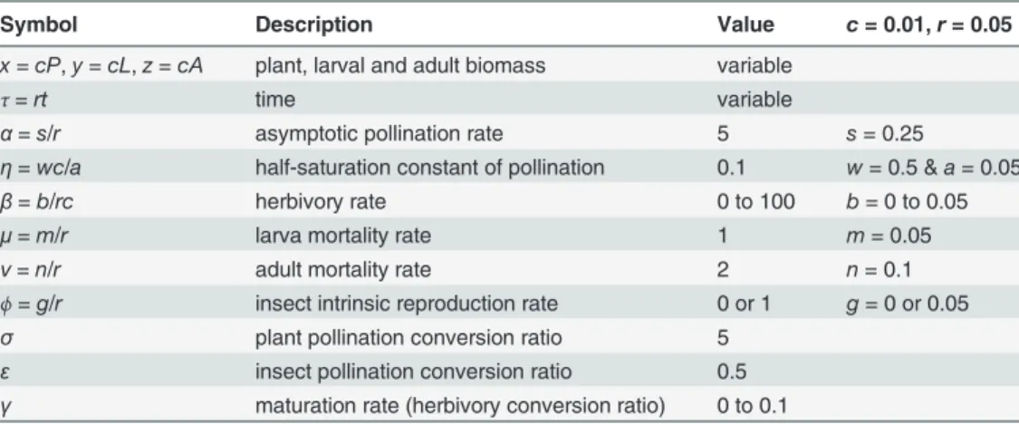
Table 1. Variables and parameters.
Symbol Description Value c= 0.01,r= 0.05
x=cP,y=cL,z=cA plant, larval and adult biomass variable
τ=rt time variable
α=s/r asymptotic pollination rate 5 s= 0.25
η=wc/a half-saturation constant of pollination 0.1 w= 0.5 &a= 0.05
β=b/rc herbivory rate 0 to 100 b= 0 to 0.05
μ=m/r larva mortality rate 1 m= 0.05
ν=n/r adult mortality rate 2 n= 0.1
ϕ=g/r insect intrinsic reproduction rate 0 or 1 g= 0 or 0.05
σ plant pollination conversion ratio 5
ε insect pollination conversion ratio 0.5
γ maturation rate (herbivory conversion ratio) 0 to 0.1
Variables and parameters of the scaled PLA model (3) and values used for numerical analyses. The last column shows a corresponding set of parameter values in the unscaled version of the same model (2), for plant carrying capacities ofc−1= 100 biomass units, andr−1= 20 time units.
Matlab [24] or GNU/Octave [25]. We also present a simplified graphical analysis of our model, in order to explain how different dynamics can arise, by varying other parameters. The source codes supporting these results are provided as supplementary material (S1 File).
Results
Numerical results
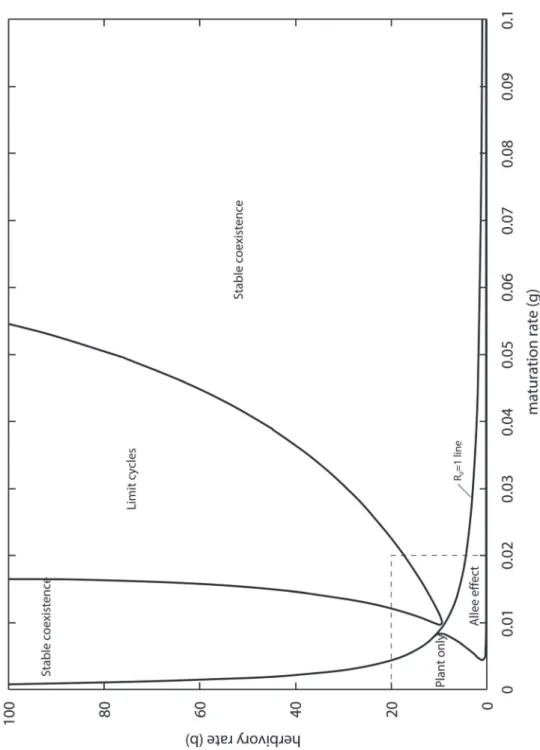
Fig. 2shows interaction outcomes of the PLA model, as a function ofβandγfor specialist pol-linators (ϕ= 0). This parameter space is divided by a decreasingRo= 1 line that indicates
whether or not insects can invade when rare.Rois defined as (see derivation inS1 File):
Ro¼
agb
ZnðmþgbÞ ð4Þ
and we call it thebasic reproductive number, according to the argument that follows. Consider the following in system (3): if the plant is at carrying capacity (x= 1), and is invaded by a very small number of adult insects (z0), the average number of larvae produced by a single adult in a given instant isεαx/(η+z)εα/η, and during its life-time (ν−1) it isεα/ην. Larvae die at the rateμ, or mature with a rate equal toγβx=γβ, per larva. Thus, the probability of larvae be-coming adults rather than dying isγβ/(μ+γβ). Multiplying the life-time contribution of an adult by this probability gives the expected number of new adults replacing one adult per gen-eration during an invasion (Ro). More formally,Rois the expected number of
adult-insect-grams replacing one adult-insect-gram per generation (assuming a constant mass-per-individ-ual ratio).
Below theRo= 1 line, small insect populations cannot replace themselves (Ro<1) and two
outcomes are possible. If the maturation rate is too low, the plant only equilibrium (x= 1,y=z = 0) is globally stable and plant–insect coexistence is impossible for all initial conditions. If the maturation rate is large enough, stable coexistence is possible, but only if the initial plant and insect biomass are large enough. This is expected in models where at least one species, here the insect, is an obligate mutualist. In this region of the space of parameters, the growth of small in-sect populations increases with population size, a phenomenon called the Allee effect [26].
Above theRo= 1 line the plant only equilibrium is always unstable against the invasion of
small insect populations (Ro>1). Plants and insects can coexist in a stable equilibrium or via
limit cycles (stable oscillations). The zone of limit cycles occurs for intermediate values of the maturation rate (γ) and it widens with rate of herbivory (β).
Plant equilibrium when coexisting with insects can be above or below the carrying capacity (x= 1). When above carrying capacity the net result of the interaction is a mutualism (+,+). While in the second case we have antagonism, more specifically net herbivory (−,+). As it
would be expected, increasing herbivory rates (β) shifts this net balance towards antagonism (low plant biomass), while decreasing it shifts the balance towards mutualism (high plant bio-mass). The quantitative response to increases in the maturation rate (γ) is more complex how-ever (see the bifurcation plot inS1 File).
entire plant cycle (maxima and minima) ends above the carrying capacity ifβis low enough (seeS1 File), but further decrease causes damped oscillations. We also found examples in which coexistence can be stable or lead to limit cycles depending on the initial conditions (see example inS1 File), but this happens in a very restrictive region in the space of parameters (see bifurcation plot inS1 File). Limit cycles can also cross the plant’s carrying capacity under the Fig 2. Outcomes of the PLA model as a function of the larval maturation and herbivory rates for specialist pollinators (ϕ= 0).The rectangular region in the bottom left is analyzed with more detail inS1 File.
original interaction mechanism (1), which does not assume the steady–state in the flowers (see S1 File, using parameters in the last column ofTable 1).
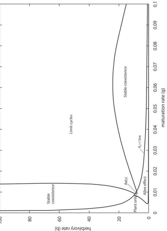
Fig. 4shows theβvsγparameter space of the model when the adults are more generalist. The relative positions of the plant-only, Allee effect, and coexistence regions are similar to the case of specialist pollinators (Fig. 2). However, the region of limit cycles is much larger. TheR0
= 1 line is closer to the origin, because the expression forR0is now (see derivation inS1 File):
R0¼
ðaþZÞgb
ZnðmþgbÞ ð5Þ
In other words, this means that the more generalist the adult pollinators (largerϕ), the more likely they can invade when rare. There is also a small overlap between the Allee effect and limit cycle regions, i.e. parameter combinations for which the long term outcome could be in-sect extinction or plant–insect oscillations, depending on the initial conditions.
Graphical analysis
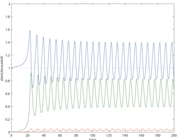
The general features of the interaction can be studied by phase-plane analysis. To make this easier, we collapsed the three-dimensional PLA model into a two-dimensional plant–larva (PL) model, by assuming that adults are extremely short lived compared with plants and larvae (see resulting ODE inS1 File). The closest realization of this assumption could beManduca sexta, Fig 3. Limit cycles in the PLA model (3).Plant biomass alternates above and below the carrying capacity (dotted line). Parameters as inTable 1, withγ= 0.01,β= 10. Blue:plant, green:larva, red:adult.
which has a larval stage of approximately 20–25 days and adult stages of around 7 days [29, 30]. For a given parametrization (Table 1), the PL model has the same equilibria as the PLA model, but not the exact same global dynamics due to the alteration of time scales. Yet, this simplification provides insights about the outcomes displayed in Figs.2and4.
Fig 4. Outcomes of the PLA model as a function of the larval maturation and herbivory rates for generalist pollinators (ϕ= 1).AeLc: intersection of the Allee effect and Limit cycle zones.
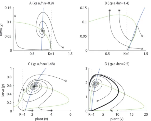
Fig. 5shows representative examples of plant and larva isoclines (i.e. non-trivial nullclines) and coexistence equilibria (intersections). Isocline properties are analytically justified (seeS1 Fileand supplemented [31] worksheet). The local dynamics around equilibria depends on the eigenvalues of the jacobian matrix of the PL model at the equilibrium. However, the highly non-linear nature of the PL model (seeS1 File), makes it pointless to try infer the signs of the eigenvalues by analytical means (except for trivial and plant-only equilibrium). Thus, we pro-pose to use to local geometry of isocline intersections to infer local stability [32]. Plant isoclines take two main forms:
gsa<Zn the isocline lies entirely belowðto the left ofÞthe carrying capacity
gsa>Zn parts of the isocline lie aboveðto the right ofÞthe carrying capacity
(
ð6Þ
In both cases, plants grow between the isocline and the axes, and decrease otherwise. Larva iso-clines are simpler, they start in the plant axis and bend towards the right when insects tend to-wards specialization (ϕ<ν), as shown byFig. 5. When insects tend towards generalism (ϕ>
ν), their isoclines increase rapidly upwards like the letter“J”(not shown here, seeS1 File). In-sects grow below and right of the larva isocline, and decrease otherwise.
Theγσα<ηνcase inFig. 5Aillustrates scenarios in which pollination rates (α), plant bene-fits (σ), adult pollinator lifetimes (1/ν) and larva-to-adult transition rates (γ) are low. The plant’s isocline is a decreasing curve crossing the plant’s axis at its carrying capacity K (x= 1,y = 0). The intersection with the larva isocline creates a globally stable equilibrium, approached by oscillations of decreasing amplitude. The local stability of this equilibrium can be explained partly by the geometry of the intersection:Fig. 5Ashows that if plants increase (decrease) above (below) the intersection point, while keeping the insect density fixed, they enter a zone of negative (positive) growth; and the same behavior holds for the insects while keeping the plants fixed. In ecological terms, both species are self-limited around the equilibrium, a strong indication of stability [32]. Together with the fact that the trivial (x= 0,y= 0) and carrying ca-pacity equilibrium (x= 1,y= 0) are saddle points, we conclude that plants and insects achieve a globally stable equilibrium after a period of transient oscillations (provided that insects are vi-able, e.g.β,γ,εare large enough). This equilibrium is demographically unfavorable for the plant because its biomass lies below the carrying capacity (x<1). Indeed, for extreme scenarios of negligible plant pollination benefits (i.e.αand/orσtend to zero), the plant’s isocline approx-imates a straight line with a negative slope, like the isocline of a logistic prey in a Lotka– Vol-terra model, which is well known to cause damped oscillations [32].
Theγσα>ηνcase inFigs. 5B,C,Dcover scenarios in which pollination rates (α), pollination benefits (σ), adult pollinator lifetimes (1/ν) and larva-to-adult (harm-to-benefit) transition rates (γ) are high. One part of the plant’s isocline lies above the carrying capacity, which means that coexistence equilibria with plant biomass larger than the carrying capacity (x>1) are pos-sible, and this is favorable for the plant.Fig. 5B, shows and example where the larva isocline in-tersects the plant’s isocline twice above the carrying capacity. One intersection is a locally stable coexistence equilibrium, whereas the other intersection is a saddle point. The saddle point belongs to a boundary that separates regions of initial conditions leading to insect persis-tence or extinction. This can explain the Allee effect, i.e. insect growth rates increase (go from negative to positive) with insect density when insect populations are very small.
of the hump (like inFig. 5C,D) are expected to result in reduced stability. This is because a small increase (decrease) along the plant’s axis leaves the plant at the growing (decreasing) side of its isocline, promoting further increase (decrease). This means that plants do not experience self-limitation, which is an indication of instability [32], and we infer that oscillations will not vanish.Fig. 5Dshows an example where an intersection at the left of the hump causes instabili-ty, leading to limit cycles. However,Fig. 5Cshows an exception of this prediction (the intersec-tion is stable). In both examples the intersecintersec-tion occurs above the plants carrying capacity, thus revealing oscillations alternating above and below the plant’s carrying capacity. We want to stress one more time, that these predictions based on isocline intersection configurations (left vs right of the hump) must be taken as“rules of thumb”.
Fig. 5Calso reveals an important consequence of the dual interaction between the plant and the insect. As we can see, the presence of a saddle point leads to the Allee effect explained be-fore. But this figure also shows that large larval densities can lead to insect extinction. This can be explained by the fact that at large initial densities, the larva overexploits the plant, and this is followed by an insect population crash from which it cannot recover due to the Allee effect. Fig 5. Dynamics of the simplified version of the PLA model.Plant isoclines in green and larva isoclines in blue. Several trajectories are shown (starting with*). The dotted line atx= 1 is the plant’s carrying capacity. Whenγσα/ην<1 the plant’s isocline always decreases, whenγσα/ην>1, it bulges above the carrying capacity and displays a hump. (A) Damped oscillations leading to globally stable coexistence dominated by antagonism (victim–exploiter). (B) The isoclines intersect as a locally stable mutualistic equilibrium and as a saddle point. Insects can coexist with the plant or go extinct depending on the initial conditions. (C) This is similar to case (B), however, a stable mutualism occurs only after damped oscillations or the insect go extinct, depending on the initial conditions. (D) Here the system develops oscillations approaching a limit cycle (thick loop), which creates a periodic alternation between mutualism and antagonism. Common parameters in all panels areβ= 10,η= 0.1,μ= 1,ϕ= 0. For the other parameters; in (A):σ= 3,ε= 0.7,α= 3,γ= 0.02,ν= 2; in (B):σ= 2.1,ε= 0.21,α= 2,γ= 0.05,ν= 1.5; in (C):σ= 3.7,ε= 0.2,α= 3,γ= 0.02,ν= 1.5; in (D):σ= 5,ε= 0.3,α= 5,γ= 0.02,ν= 2.
Asγ,σ,αincrease and/orη,νdecrease more and more, the decreasing segment of the plant isocline (the part at the right of the hump) approximates a decreasing line (actually a straight asymptotic line, seeS1 File), while the rest of the isocline is pushed closer and closer to the axes. In other words, when pollination rates (α), benefits (σ), adult lifetimes (1/ν) and larva de-velopment rates (γ) increase, plant isoclines would resemble the isocline of a logistic prey, with a“pseudo”carrying capacity (the rightmost extent of the isocline) larger than the intrinsic car-rying capacity (x= 1).Fig. 5Dis an example of this. These conditions would promote stable co-existence with large plant equilibrium biomasses.
Discussion
We developed a plant–insect model that considers two interaction types, pollination and her-bivory. Ours belongs to a class of models [33,34] in which balances between costs and benefits cause continuous variation in interaction strengths, as well as transitions among interaction types (mutualism, predation, competition). In our particular case, interaction types depend on the stage of the insect’s life cycle, as inspired by the interaction betweenM. sextaandD. wrightii[6,14] or betweenM. sextaandN. attenuata[10]. There are many other examples of pollination–herbivory in Lepidopterans, where adult butterflies pollinate the same plants ex-ploited by their larvae [5,7]. We assign antagonistic and mutualistic roles to larva and adult in-sect stages respectively, which enable us to study the consequences of ontogenetic changes on the dynamics of plant–insect associations, a topic that is receiving increased attention [8,17]. Our model could be generalized to other scenarios, in which drastic ontogenetic niche shifts cause the separation of benefits and costs in time and space. However, it excludes cases like the yucca/yucca moth interaction [35] where adult pollinated ovules face larval predation, i.e. ben-efits themselves are deducted.
Instead of using species biomasses as resource and service proxies [34], we consider a mech-anism (1) that treats resources more explicitly [36]. We use flowers as a direct proxy of resource availability, by assuming a uniform volume of nectar per flower. Nectar consumption by insects is concomitant with service exploitation by the plants (pollination), based on the assumption that flowers contain uniform numbers of ovules. Pollination also leads to flower closure [19], making them limiting resources. Flowers are ephemeral compared with plants and insects, so we consider that they attain a steady-state between production and disappearance. As a result, the dynamics is stated only in terms of plant, larva and adult populations, i.e. the PLA model (3). The feasibility of the results described by our analysis depends on several parameters. The consumption, mortalities and growth rates, and the carrying capacities (e.g.a,b,m,nand r,cin the fourth column ofTable 1), have values close to the ranges considered by other models [34,37]. Oscillations, for example, require large herbivory rates, but this is usual for M. sexta[15].
Mutualism
–
antagonism cycles
The PLA model displays plant–insect coexistence for any combination of (non-trivial) initial conditions where insects can invade when rare (Ro>1). Coexistence is also possible where
in-sects cannot invade when rare (Ro<1), but this requires high initial biomasses of plants and
insects (Allee effect). Coexistence can take the form of a stable equilibrium, but it can also take the form of stable oscillations, i.e. limit cycles.
cycles require herbivory rates (β) to be large enough. Second, given limit cycles, an increase in the maturation rate (γ) causes a transition to stable coexistence, and further increase in herbiv-ory is required to induce limit cycles again (Fig. 2). This makes sense because by speeding up the transition from larva to adult, the total effect of herbivory on the plants is reduced, hence preventing a crash in plant biomass followed by a crash in the insects. Third, when adult polli-nators have alternative food sources (ϕ>1), the zone of limit cycles in the space of parameters becomes larger (Fig. 4). This also makes sense, because the total effect of herbivory increases by an additional supply of larva (which is not limited by the nectar of the plant considered), lead-ing to a plant biomass crash followed by insect decline.
The graphical analysis provides another indication that oscillations are herbivory driven. On the one hand insect isoclines (or rather larva isoclines) are always positively sloped, and in-sects only grow when plant biomass is large enough (how large depends on insect’s population size, due to intra-specific competition). Plant isoclines, on the other hand, can display a hump (Fig. 5B,C,D), and they grow (decrease) below (above) the hump. These two features of insect and plant isoclines are associated with limit cycles in classical victim–exploiter models [27]. If there is no herbivory or another form of antagonism (e.g. competition) but only mutualism, the plant’s isocline would be a positively sloped line, and plants would attain large populations in the presence of large insect populations, without cycles. However, mutualism is still essential for limit cycles: if mutualistic benefits are not large enough (γσα<ην), plant isoclines do not have a hump (Fig. 5A) and oscillations are predicted to vanish. The effect of mutualism on sta-bility is like the effect of enrichment on the stasta-bility in pure victim–exploiter models [28], by al-lowing the plants to overcome the limits imposed by their intrinsic carrying capacity.
There is a minorcaveatregarding our graphical analysis: whereas a hump in the plant’s iso-cline is a requisite for oscillations to evolve into limit cycles, this does not mean that isoiso-cline in-tersections at the left of the hump always lead to limit cycles (Fig. 5C). To our best knowledge, this always happens only for quite specific conditions in pure victim–exploiter models [40]. As long as we cannot prove by analytical means that intersection geometry determines local stabil-ity, the prediction of limit cycles remains a“rule of thumb”, based on extrapolating our knowl-edge about other victim–exploiter models.
Classification of outcomes: mutualism or herbivory?
Interactions can be classified according to the net effect of one species on the abundance (bio-mass, density) of another (but see other schemes [41]). This classification scheme can be prob-lematic in empirical contexts because reference baselines such as carrying capacities are usually not known [42].
Our PLA model illustrates the classification issue when non-equilibrium dynamics are gen-erated endogenously, i.e. not by external perturbations. Since plants are facultative mutualists and insects are obligatory ones, one can say the outcome isnet mutualism(+,+) ornet herbivo-ry(−,+), if the coexistence is stable, and the plant equilibrium ends up respectively above or
below the carrying capacity [33,34]. If coexistence is under non-equilibrium conditions and plant oscillations are entirely below the carrying capacity (e.g. for large herbivory rates), the outcome is detrimental for plants and hence there is net herbivory (−,+); oscillations may in
mutualism due to enlarged plant biomasses, but the oscillations indicates that a victim– exploit-er intexploit-eraction exists. As we can see, deciding upon the net outcome require considexploit-eration of both equilibrium and dynamical aspects.
Factors that could cause dynamical transitions
Environmental factors. The parameters in our analyses can change due to external fac-tors. One of the most important is temperature [43]. It is well known, for example, that climate warming can reduce the number of days needed by larvae to complete their development [44], making larvae maturation rates (γ) higher. For insects that display Allee effects, a cooling of the environment will cause the sudden extinction of the insect and a catastrophic collapse of the mutualism, which cannot be simply reverted by warming. By retarding larva development into adults, cooling would increase the burden of herbivory over the benefits of pollination, making the system less stable by promoting oscillations. Flowering, pollination, herbivory, growth and mortality rates (e.g.s,a,b,r,mandnin equations1) are also temperature-dependent and they can increase or decrease with warming depending on the thermal impacts on insect and plant metabolisms [45]. This makes general predictions more difficult. However, we get the general picture that warming or cooling can change the balance between costs and benefits impacting the stability of the plant–insect association.
Dynamical transitions can also be induced by changes in the chemical environment, often as a consequence of human activity. Some pesticides, for example, are hormone retarding agents [46]. This means that their release can reduce maturation rates, altering the balance of the interaction towards more herbivory and less pollination and finally endangering pollina-tion service [47,48]. In other cases, the chemical changes are initiated by the plants: in response to herbivory, many plants release predator attractants [49], which can increase larval mortality (μ). If the insect does nothing but harm, this is always an advantage. If the insect is also a very effective pollinator, the abuse of this strategy can cost the plant important pollination services because a dead herbivore today is one less pollinator tomorrow.
Another factor that can increase or decrease larvae maturation rates, is the level of nutrients present in the plant’s vegetative tissue [50,51]. On the one hand, the use of fertilizers rich in phosphorus could increase larvae maturation rates [51]. On the other hand, under low protein consumptionM. sextalarvae could decrease maturation rate, althoughM. sextalarvae can compensate this lack of proteins by increasing their herbivory levels (i.e. compensatory con-sumption) [50]. Thus, different external factors related to plant nutrients could indirectly trig-ger different larvae maturation rates that will potentially modify the interaction dynamics.
Pollinator’s diet breadth. An important factor that can affect the balance between mutu-alism and herbivory is the diet breadth of pollinators. Alternative food sources for the adults could lead to apparent competition [52] mediated by pollination, as predicted for the interac-tion betweenD. wrigthii(Solanacea) andM. sexta(Sphingidae) in the presence ofAgave pal-mieri(plant) [6]: visitation ofAgavebyM. sextadoes not affect the pollination benefits received byD. wrightii, but it increases oviposition rates onD.wrightii, increasing herbivory. As discussed before, such an increase in herbivory could explain why oscillations are more widespread when adult insects have alternative food sources (ϕ>0) in our PLA model.
community modules or networks, taking into account that there is a positive correlation be-tween the diet breadths of larval and adult stages [7].
From the perspective of the plant, the lack of alternative pollinators could also lead to in-creased herbivory and loss of stability. The case of the tobacco plant (N. attenuata) andM. sextais illustrative. These moths are nocturnal pollinators, and in response to herbivory by their larvae, the plants can change their phenology by opening flowers during the morning in-stead. Thus, oviposition and subsequent herbivory can be avoided, whereas pollination can still be performed by hummingbirds [11]. Although hummingbirds are thought to be less reliable pollinators than moths for several reasons [9], they are an alternative with negligible costs. Thus, a decline of hummingbird populations will render the herbivore avoidance strategy use-less and plants would have no alternative but to be pollinated by insects with herbivorous lar-vae that promote oscillations.
Conclusions
Many insect pollinators are herbivores during their larval phases. If pollination and herbivory targets the same plant (e.g. as between tobacco plants and hawkmoths), the overall outcome of the association depends on the balance between costs and benefits for the plant. As predicted by our plant-larva-adult (PLA) model, this balance is affected by changes in insect develop-ment: the faster larvae turns into adults the better for the plant and the interaction is more sta-ble; the slower this development the poorer the outcome for the plant and the interaction is less stable (e.g. oscillations). Under plant–insect oscillations, this balance can be dynamically com-plex (e.g. periodic alternation between mutualism and antagonism). Since maturation rates play an essential role in long term stability, we predict important qualitative changes in the dy-namics due to changes in environmental conditions, such as temperature and chemical com-pounds (e.g. toxins, hormones, plant nutrients). The stability of these mixed interactions can also be greatly affected by changes in the diet generalism of the pollinators.
Supporting Information
S1 File. Supplement containing the appendices cited in the main text.
(PDF)
S1 Fig. Detail of theβvsγparameter space for specialist pollinators in the PLA model.The ellipse describes the joint variation ofγandβtaking place in the bifurcation diagram inS2 Fig. (EPS)
S2 Fig. Bifurcation diagram for the PLA model.Parametersγandβvary along the elliptical path drawn inS1 Fig, with reference for each quarter of a rotation. Solid (broken) lines repre-sent stable (unstable) equilibria, black (white) circles reprerepre-sent limit cycle maxima and minima. Thex= 1 line corresponds to the plant carrying capacity.HBsuper: super-critical andHBsub:
sub-critical Hopf bifurcations, BP: branching point (transcritical bifurcation), LP: limit point (fold bifurcation).
(EPS)
S3 Fig. Main configurations of the plant isocline.We only consider the O–K segment in the positive octant (hatched square). In A the isocline lies below the plant’s carrying capacity (i.e. left of K), in B parts of the isocline lie above (i.e. right of K).
(EPS)
form of a mushroom. (B) Asβincreases, O, P, Q and the diagonal asymptote move towards the plant axis and the isocline is compressed vertically.
(EPS)
S5 Fig. Main configurations of the larva isocline.The isocline consists of three black lines, but only the segment in the positive octant (hatched square) is biologically relevant. For A and Bϕ<ν. For C and Dϕ>ν. The green parabolap(x) is the numerator of the isocline and the circles indicate its roots, wherex0: positive root. The red parabolaq(x) is the denominator of
the isocline, which has two rootsx= 0 andx=xv, both of which are also the vertical asymptotes
of the isocline. The isocline also has an horizontal asymptoteyh. The alternative in part D can
be dismissed because it implies a detrimental effect of plants on insects. (EPS)
S6 Fig. Shape of the larva isocline.(A) Forϕ<νthe larva isocline moves closer to the larva axis and becomes more shallow asγandβincrease. (B) Forϕ>νthe larva isocline becomes closer to the larva axis.
(EPS)
S7 Fig. Plant oscillating above their carrying capacity in the PLA model.Blue:plant, green: larva, red:adult. The carrying capacity is indicated by the dotted line.
(EPS)
S8 Fig. Oscillations in the PLA model started with different initial conditions ().The
oscil-lations can dampen out (blue) or converge to a limit cycle (red). (EPS)
S9 Fig. Interaction dynamics when flowers are explicitly considered.Blue:plant, green:larva, red:adult, black:flowers. The dotted line indicates the plant’s carryng capacity.
(EPS)
Acknowledgments
We thank Rampal Etienne for the discussions that inspired us to write this article. We thank the comments and suggestions from our colleagues of the Centre for Biodiversity Theory and Modelling in Moulis, France, the Centre for Australian National Biodiversity and Research at CSIRO in Canberra, Australia, and two anonymous reviewers.
Author Contributions
Conceived and designed the experiments: TAR FEV. Performed the experiments: TAR. Ana-lyzed the data: TAR. Contributed reagents/materials/analysis tools: TAR. Wrote the paper: TAR FEV.
References
1. Bronstein J, Alarcón R, Geber M (2006) Tansley review: evolution of plant-insect mutualisms. New Phy-tologist 172: 412–428. doi:10.1111/j.1469-8137.2006.01864.xPMID:17083673
2. Jones E, Bronstein J, Ferriere R (2012) The fundamental role of competition in the ecology and evolu-tion of mutualisms. Annals of the New York Academy of Sciences 1256: 66–88. doi:
10.1111/j.1749-6632.2012.06552.xPMID:22583047
3. Bronstein JL (1994) Conditional outcomes in mutualistic interactions. Trends in Ecology and Evolution 9: 214–217. doi:10.1016/0169-5347(94)90246-1PMID:21236825
5. Wäckers FL, Romeis J, van Rijn P (2007) Nectar and pollen feeding by insect herbivores and implica-tions for multitrophic interacimplica-tions. Annual Review of Entomology 52: 301–323. doi:10.1146/annurev.
ento.52.110405.091352PMID:16972766
6. Bronstein JL, Huxman T, Horvath B, Farabee M, Davidowitz G (2009) Reproductive biology of Datura wrightii: the benefits of a herbivorous pollinator. Annals of Botany 103: 1435–1443. doi:10.1093/aob/
mcp053PMID:19287014
7. Altermatt F, Pearse IS (2011) Similarity and specialization of the larval versus adult diet of european butterflies and moths. American Naturalist 178: 372–382. doi:10.1086/661248PMID:21828993 8. Rudolf VHW, Lafferty KD (2011) Stage structure alters how complexity affects stability of ecological
net-works. Ecology letters 14: 75–79. doi:10.1111/j.1461-0248.2010.01558.xPMID:21114747 9. Irwin RE (2010) Evolutionary ecology: when pollinators are also herbivores. Current Biology 20: 100–
101. doi:10.1016/j.cub.2009.12.005
10. Baldwin IT (1988) The alkaloidal responses of wild tobacco to real and simulated herbivory. Oecologia 77: 378–381. doi:10.1007/BF00378046
11. Kessler D, Diezel C, Baldwin IT (2010) Changing pollinators as a means of escaping herbivores. Cur-rent Biology 20: 237–242. doi:10.1016/j.cub.2009.11.071PMID:20096581
12. Kennedy G (2003) Tomato, pests, parasitoids, and predators: Tritrophics interactions involving the Genus Lycopersicon. Annual Review of Entomology 48: 51–72. doi:10.1146/annurev.ento.48.
091801.112733PMID:12194909
13. Campbell C, Walgenbach J, Kennedy G (1991) Effect of Parasitoids on Lepidopterous Pests in Insecti-cide-Treated and Untreated Tomatoes in Western North Carolina. Journal of Economic Entomology 84: 1662–1667. doi:10.1093/jee/84.6.1662
14. Alarcon R, Davidowitz G, Bronstein JL (2008) Nectar usage in a southern Arizona hawkmoth communi-ty. Ecological Entomology 33: 503–509. doi:10.1111/j.1365-2311.2008.00996.x
15. McFadden M (1968) Observations on feeding and movement of tobacco hornworm larvae. Journal of Economic Entomology 61: 352–356. doi:10.1093/jee/61.2.352
16. Barron-Gafford G, Rascher U, Bronstein J, Davidowitz G, Chaszar B, et al. (2012) Herbivory of wild Manduca sextacauses fast down-regulation of photosynthetic efficiency inDatura wrightii: an early sig-naling cascade visualized by chlorophyll fluorescence. Photosynthesis Research 113: 249–260. doi:
10.1007/s11120-012-9741-xPMID:22576017
17. Miller TEX, Rudolf VHW (2011) Thinking inside the box: community-level consequences of stage-struc-tured populations. Trends in Ecology and Evolution 26: 457–466. doi:10.1016/j.tree.2011.05.005 PMID:21680049
18. Hunt WF, Loomis RS (1976) Carbohydrate-limited growth kinetics of tobacco (Nicotiana rustica L.) cal-lus. Plant Physiology 57: 802–805. doi:10.1104/pp.57.5.802PMID:16659573
19. Primack RB (1985) Longevity of individual flowers. Annual Review of Ecology and Systematics 16: 15– 37. doi:10.1146/annurev.es.16.110185.000311
20. Rinaldi S, Scheffer M (2000) Geometric analysis of ecological models with slow and fast processes. Ecosystems 3: 507–521. doi:10.1007/s100210000045
21. Schoener TW (1978) Effects of density-restricted food encounter on some singlelevel competition mod-els. Theoretical Population Biology 13: 365–381. doi:10.1016/0040-5809(78)90052-7PMID:734620 22. Fagan WF, Bewick S, Cantrell S, Cosner C, Varassin IG, et al. (2014) Phenologically explicit models for
studying plant-pollinator interactions under climate change. Theoretical Ecology 7: 289–297. doi:10. 1007/s12080-014-0218-8
23. Ermentrout B (2003) XPPAUT 5.41—The differential equations tool. University of Pittsburgh. URL http://www.math.pitt.edu/~bard/xpp/xpp.html
24. MATLAB (2010) version 7.14.0 (R2012a). Natick, Massachusetts: The MathWorks Inc.
25. Eaton JW, Bateman D, Hauberg S (2008) GNU Octave Manual Version 3. Network Theory Ltd. URL https://www.gnu.org/software/octave/
26. Stephens PA, Sutherland WJ, Freckleton RP (1999) What is the Allee effect? Oikos 87: 185–190. doi: 10.2307/3547011
27. Rosenzweig ML, MacArthur RH (1963) Graphical representation and stability conditions of predator-prey interactions. American Naturalist 97: 209–223. doi:10.1086/282272
28. Rosenzweig ML (1971) The paradox of enrichment. Science 171: 385–387. doi:10.1126/science.171.
3969.385PMID:5538935
30. Ziegler R (1991) Changes in lipid and carbohydrate metabolism during starvation in adultManduca sexta. Journal of Comparative Physiology B 161: 125–131. doi:10.1007/BF00262874
31. Mathematica (2010) version 8.0. Champaign, Illinois: Wolfram Research, Inc. 32. Case T (2000) An Illustrated Guide to Theoretical Ecology. Oxford University Press.
33. Hernandez MJ (1998) Dynamics of transitions between population interactions: a nonlinear interaction
α-function defined. Proceedings of the Royal Society B: Biological Sciences 265: 1433–1440. doi:10.
1098/rspb.1998.0454
34. Holland JN, DeAngelis DL (2010) A consumer-resource approach to the densitydependent population dynamics of mutualism. Ecology 91: 1286–1295. doi:10.1890/09-1163.1PMID:20503862
35. Holland JN, DeAngelis DL, Bronstein JL (2002) Population dynamics and mutualism: functional re-sponses of benefits and costs. American Naturalist 159: 231–244. doi:10.1086/338510PMID: 18707376
36. Encinas-Viso F, Revilla TA, Etienne RS (2014) Shifts in pollinator population structure may jeopardize pollination service. Journal of Theoretical Biology 352: 24–30. doi:10.1016/j.jtbi.2014.02.030PMID: 24607744
37. Johnson CA, Amarasekare P (2013) Competition for benefits can promote the persistence of mutualis-tic interactions. Journal of Theoremutualis-tical Biology 328: 54–64. doi:10.1016/j.jtbi.2013.03.016PMID: 23542049
38. Wang Y, Deangelis DL (2012) A mutualism-parasitism system modeling host and parasite with mutual-ism at low density. Mathematical Biosciences and Engineering 9: 431–444. doi:10.3934/mbe.2012.9. 431PMID:22901072
39. Holland JN, Wang Y, Sun S, DeAngelis DL (2013) Consumer-resource dynamics of indirect interactions in a mutualism-parasitism food web module. Theoretical Ecology 6: 475–493. doi: 10.1007/s12080-013-0181-9
40. Freedman HI (1976) Graphical stability, enrichment, and pest control by a natural enemy. Mathematical Biosciences 31: 207–225. doi:10.1016/0025-5564(76)90080-8
41. Abrams PA (1987) On classifying interactions between populations. Oecologia 73: 272–281. doi:10. 1007/BF00377518
42. Hernandez MJ (2009) Disentangling nature, strength and stability issues in the characterization of pop-ulation interactions. Journal of Theoretical Biology 261: 107–119. doi:10.1016/j.jtbi.2009.07.001 PMID:19589344
43. Gillooly JF, Brown JH, West GB, Savage VM, Charnov EL (2001) Effects of size and temperature on metabolic rate. Science 293: 2248–2251. doi:10.1126/science.1061967PMID:11567137
44. Bonhomme R (2000) Bases and limits to using‘degree.day’units. European Journal of Agronomy 13: 1–10. doi:10.1016/S1161-0301(00)00058-7
45. Vasseur DA, McCann KS (2005) Mechanistic approach for modeling temperaturedependent consum-er-resource dynamics. American Naturalist 166: 184–198. doi:10.1086/431285PMID:16032573 46. Dev S (1986) Trends in development of insect growth regulators in plant protection. Proceedings of the
Indian National Science Academy B52: 17–24.
47. Potts S, Biesmeijer J, Kremen C, Neumann P, Schweiger O, et al. (2010) Global pollinator declines: trends, impacts and drivers. Trends in Ecology and Evolution 25: 345–353. doi:10.1016/j.tree.2010.
01.007PMID:20188434
48. Kearns C, Inouye D, Waser N (1998) Endangered mutualims: The conservation of plant-pollinator Inter-actions. Annual Review of Ecology and Systematics 29: 83–112. doi:10.1146/annurev.ecolsys.29.1. 83
49. Allmann S, Baldwin IT (2010) Insects betray themselves in nature to predators by rapid isomerization of green leaf volatiles. Science 329: 1075–1078. doi:10.1126/science.1191634PMID:20798319 50. Woods H (1999) Patterns and Mechanisms of Growth of Fifth-InstarManduca sextaCaterpillars
Follow-ing Exposure to Low- or High-Protein Food durFollow-ing Early Instars. Physiological and Biochemical Zoology 72: 445–454. doi:10.1086/316678PMID:10438682
51. Perkins M, Woods H, Harrison J, Elser J (2004) Dietary Phosphorus Affects the Growth of Larval Man-duca sexta. Archives of Insect Biochemistry and Physiology 53: 153–168. doi:10.1002/arch.10133 52. Holt RD (1977) Predation, apparent competition, and the structure of prey communities. Theoretical