Back to basics: can we improve the OLS CAPM?
Alexandre Serra 152414042
Supervisor: Professor Joni Kokkonen
Dissertation submitted in partial fulfilment of requirements for the degree of Master of Science in Finance, at Universidade Católica Portuguesa, January 2016
i
Back to basics: can we improve the OLS CAPM?
Alexandre Serra Abstract
We provide empirical evidence of negative effects caused by endogeneity, associated with the estimation of the Capital Asset Pricing Model (CAPM) using Ordinary Least Squares (OLS), in 11 equity markets. We propose the implementation of two methods to estimate this model – Instrumental Variables (IV) and Two-Step Least Squares (2SLS). The results show that the betas obtained by using 2SLS can significantly predict future market returns a higher percentage of times than the OLS and IV approach. The 2SLS estimates also show a higher forecasting power over the future returns of the own stock.
Abstrato
Apresentamos provas empíricas de efeitos negativos causados pela endogeneidade, associados à estimação da CAPM utilizando o Método dos Mínimos Quadrados (MMQ), em 11 mercados. Propomos a implementação de dois métodos para a estimação deste modelo – Variáveis Instrumentais (VI) e Mínimos Quadrados em 2 Estágios (MQ2E). Os resultados demonstram que os betas obtidos através de MQ2E conseguem prever significativamente futuros retornos do mercado uma maior percentagem das vezes que a abordagem de MMQ ou VI. As estimativas do MQ2E também mostram um maior poder de previsão sobre os futuros retornos da própria ação.
ii Acknowledgments
First of all, I would like to thank my supervisor Joni Kokkonen for the continuous support over the past five months. His knowledge and experience proved to be essential for me to both successfully complete tasks associated with the realization of this thesis, and to transform some of my ideas into specific financial analyses.
Secondly, I would like to thank Leonor Modesto and Patrícia Cruz for their support and clarifications regarding econometric problems I needed to solve in order to complete my thesis. Thirdly, I would like to thank my Empirical Finance group, Catarina Ribeiro, Filipe Tavares and Rita Carvalho, as well as Professor José Faias, who taught me habits and skills that made the investigation process and writing of this thesis much easier.
I would also like to thank all of my friends who helped and motivated me, not only through the thesis semester, but during my entire Masters at Católica, both in and out of classes. A special thanks to Manel, Miguel, Duarte, Nuno, Mónica, Francisco Conde, Ricardo Santos, and Catarina Oliveira.
Finally, I would like to thank my parents for putting the effort to support me through these two years, and for giving me the opportunity to complete this prestigious program.
iii Table of contents 1. Introduction ... 1 2. Data ... 4 3. Methodology ... 5 3.1. Estimation methods ... 6
3.2. Analysing the estimates ... 11
4. Empirical Analysis ... 14
4.1. In-sample results ... 14
4.2. Out-of-sample results ... 19
5. Conclusion ... 23
1 1. Introduction
The estimation of parameters such as the beta of a given stock or the cost of equity of a company is a step of crucial importance to correctly value financial assets or projects. Despite the evolution of more advanced technical models, which rely heavily on quantitative analysis, a simple CAPM estimated using OLS is still relied upon by a dominant portion of managers and investors as the model responsible for their estimates of expected returns and cost of equity. This fact is confirmed by several authors, who find that, even among prestigious companies as the ones part of Fortune 500 large firms or Forbes 200 best small companies, CAPM is the preferred model to estimate parameters such as the Weighted Average Cost of Capital (WACC) (Bruner, Eades, Harris, and Higgins, 2001). This is understandable given the simplicity of the model. As a single-factor model, it requires few inputs, and its interpretation is very straightforward since it only considers one risk factor. The model states that the return of a company depends on its sensitivity to the return of the market. This parameter is commonly referred to as beta.
Alternatively, multifactor models take into account several risk factors and try to come up with more accurate estimations of expected returns. By considering various dynamics that can influence the price of the asset, the investor is able to better understand the mechanics behind the behaviour of financial markets. For example, the Fama French 3-factor model (Fama and French, 1993) adds to the already existent market risk premium the factors of value and size, while the Carhart 4-factor model (Carhart, 1997) adds to these the momentum factor. These models have allowed for increases in the efficiency of estimations, and, at the same time, created opportunities for different investment strategies to be developed, based on earning the premiums associated with these risk factors. However, the amount of data required for its estimations, along with the associated estimation error, have caused these models to be outperformed by simpler models. In fact, MacKinlay (1995) shows that “multifactor pricing models alone do not entirely resolve CAPM deviations”. This is an interesting result in favour of the CAPM enthusiasts, since it implies that, in an ex-ante scenario, the errors committed by CAPM due to omitted risk factors, like value or momentum, are not actually explained in totality by these multifactor models.
Despite being easy to implement, the theoretical restrictions of the CAPM prevent it from always being applied in the more correct way. Bartholdy and Peare (2003) mention that a common practice found in companies seems to be the estimation of the market risk premium
2 using one index as reference, while beta, whether it is independently obtained or estimated within the company, is based on a different index. The authors find that using two different proxies for the world market portfolio in this way biases the estimations of expected return. This can have numerous consequences regarding asset allocation exercises, for instance, calculating weights for a given exposure or computing a wrong benchmark performance of an asset.
The investigation we propose in this thesis challenges one of the key assumptions of the model. Since the world market portfolio is unobservable, we must use a proxy, which is generally a market index, more specifically, the market where the stock is listed. This proxy is used to estimate the expected return of a given company. What happens then if the return of the company significantly affects the return of the market? If we are in the presence of smaller markets, where companies are not considered to be atomistic, the main consequence is that the proxy that we are using is no longer exogenous, and the model will suffer from endogeneity problems. Given that we are estimating the model using OLS, our estimates will be biased and no longer be consistent nor valid. This can be an explanation for why CAPM estimates tend to struggle in predicting returns or market risk premiums. Lai and Stohs (2015) analyse this property and go as far as saying the model is “dead”. They report that endogeneity is one of the main causes regarding the “difficulties with obtaining reliable betas or costs of capital”. In addition, they discuss the problems related with finding a good proxy for the market portfolio. In another study, Somerville and O’Connell (2002) report that the “location of the mean-variance efficient frontier of risky assets is endogenous”. Once again, this finding invalidates assumptions that make the CAPM such a simple model, and can also explain why the model tends to perform poorly out-of-sample.
With this in mind, we suggest the implementation of two more sophisticated methods, IV and 2SLS, to estimate the CAPM. Contrary to OLS, these methods are able to estimate efficiently in the presence of endogenous regressors. They require more calculations and data than OLS, but, at the same time, are not complex enough to prevent most investors or companies from estimating them. More specifically, they require the use of instruments, which are variables that should be correlated with the endogenous regressor, but, at the same time, be uncorrelated with the error term of the original regression. By using these instruments to estimate values for the endogenous regressor, we are able to eliminate any endogeneity effects, considering that the instruments fulfil the two requirements mentioned above. We opt to use the returns of other market indexes as instruments, given that, with 12 indexes in our sample, we are able to select
3 instruments with high correlations, in order to guarantee more efficient estimations. Previous authors, such as Amano, Kato and Taniguchi (2012), show that OLS estimates become inconsistent due to the dependence of the error term, but, similarly to our approach, suggest the use of 2SLS as an alternative to estimate the model when “the returns of the individual asset and error process are long-memory dependent”.
Despite the advantages in eliminating endogeneity, estimating through IV and 2SLS has its drawbacks, mainly finding appropriate instruments. Hahn and Hausman (2003) approach this issue and find that, in the presence of weak instruments, the 2SLS estimations perform poorly and, even though the OLS estimates continue to be inconsistent and biased, they are still preferable to 2SLS, given the large estimation error of the latter.
Our results show that 2SLS is able to significantly decrease endogeneity effects by providing more efficient estimates of the CAPM. This method is able not only to significantly predict market returns more often than OLS, but also with a higher R-squared, in most of the indexes included in this analysis. 2SLS manages to outperform OLS in most of the measures computed, yielding the best overall results in efficiency and predictability. These results are in accordance with our initial hypothesis and empirically confirm the existence of endogeneity effects regarding the OLS CAPM, which can be overcome by opting for the appropriate estimation methods. Additionally, they support the choice of the returns of other markets as good instruments, given that the estimation error occurred in is low enough to allow for efficiency gains. This methodology is able make our estimations more consistent, by increasing their accuracy and predictive ability.
The remainder of the thesis is organised in the following way. Section 2 presents the data used in this study. Section 3 reports the methodology followed. In section 4 we report the results of our empirical analysis. Conclusions are presented in section 5.
4 2. Data
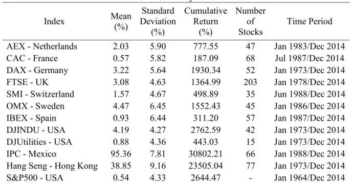
We use Thomson Reuters Datastream to extract monthly prices of companies in eleven indexes – AEX (Netherlands), CAC (France), DAX (Germany), FTSE (United Kingdom), SMI (Switzerland), OMX (Sweden), IBEX (Spain), Dow Jones Industrials and Dow Jones Utilities (USA), IPC (Mexico), and Hang Seng (Hong Kong) – for the longest period available. Additionally, we extract the prices of these indexes, with the addition of the S&P 500. Summary statistics concerning each index used in our sample are presented in Table 1. The table shows the values for the mean return, standard deviation, and cumulative return of each of the 12 indexes. The last two columns report the number of stocks analysed in each index, as well as the time period for which they are available.
Table 1 - Summary Statistics Index Mean (%) Deviation Standard
(%) Cumulative Return (%) Number of
Stocks Time Period
AEX - Netherlands 2.03 5.90 777.55 47 Jan 1983/Dec 2014
CAC - France 0.57 5.82 187.09 68 Jul 1987/Dec 2014
DAX - Germany 3.22 5.64 1930.34 52 Jan 1973/Dec 2014
FTSE - UK 3.08 4.63 1364.99 203 Jan 1978/Dec 2014
SMI - Switzerland 1.57 4.67 498.89 35 Jun 1988/Dec 2014
OMX - Sweden 4.47 6.45 1552.43 45 Jan 1986/Dec 2014
IBEX - Spain 0.93 6.44 311.20 57 Jan 1987/Dec 2014
DJINDU - USA 4.19 4.27 2762.59 42 Jan 1973/Dec 2014
DJUtilities - USA 0.88 4.36 443.03 15 Jan 1973/Dec 2014
IPC - Mexico 95.36 7.81 30802.21 66 Jan 1988/Dec 2014
Hang Seng - Hong Kong 38.85 9.16 23505.04 77 Jan 1973/Dec 2014
S&P500 - USA 0.54 4.33 2644.47 - Jan 1964/Dec 2014
To clean the data, we restrict our sample to companies with a number of observations equal to or larger than 70. This procedure is necessary in order to make sure that the number of observations is sufficient for the estimation methods to be valid, and to guarantee a minimum number of observations in the outputs of the estimations, so that we can properly analyse the results. No restrictions are made regarding the prices of the stocks, given that the goal of this Table 1. Summary Statistics – Reported are summary statistics regarding the 12 indexes included in our sample. We present the mean monthly return, standard deviation and cumulative return relative to each index. We also provide information regarding the number of stocks analysed in each index and the time period for which they are available. Returns and standard deviations are presented in percentage points.
5 thesis is to focus on smaller markets, which normally include many stocks with low prices. After applying the restrictions to our data, our final sample consists of 707 stocks in the 11 indexes.
The time frame and number of companies varies amongst indexes. In order to account for survivorship bias, whenever possible, the sample of each index contains both live companies and companies that are no longer part of the respective index. Regarding the results of these summary statistics, we can spot two indexes as outliers – IPC from Mexico and Hang Seng from Hong Kong. While the mean monthly return for the remainder of the indexes ranges from 0.54% to 4.47%, these two indexes show a mean monthly return of 95.36% and 38.85%, respectively. It is possible that the results of our estimations are different for these two indexes, as well as any general conclusions. Apart from these, the values for cumulative return, mean return and standard deviation are very disperse among all indexes with no other outliers. The number of stocks is also very different for each index, with the highest number being registered by FTSE at 203. Since this sample is much larger than the average, the results obtained by the estimations in this index can be an indicator of to what an extent the gains in efficiency exist regarding the hypothesis of endogeneity and atomicity of a company. On the other hand, if the results are favourable for the majority of the indexes, we can establish that there are efficiency gains which can be obtained by dealing with endogeneity both in these indexes and, likely, on indexes not present in our sample but of similar size.
3. Methodology
This section is divided in two parts. In the first part, we explain the methodology followed regarding the estimation procedures. After that, we provide more details regarding the methods used to evaluate the estimates obtained.
6 3.1. Estimation methods
Regarding the estimation processes, we estimate the following model, for all three estimation methods:
𝑟𝑖,𝑡 = 𝛼𝑖,𝑡+ 𝛽𝑖,𝑡 ∗ 𝑟𝑀,𝑡+ 𝜀𝑖,𝑡 (1)
The model, which is a simple variation of the standard CAPM, states that the return of a stock, at any given time, depends on the sensitivity of this asset to the market return, 𝛽, plus a constant, 𝛼, and an error term, 𝜀. This model was first introduced in the early 1960’s with several authors publishing papers on the matter – Sharpe (1964), Lintner (1965), and Mossin (1966). Since then, it has become a benchmark model used by both companies and investors when assessing issues such as calculating the expected return of an asset, computing the cost of capital of a company, or understanding how the value of a given asset changes with the return of the market. Contrary to CAPM, raw returns are used in this formula. This approach is based on Bartholdy and Peare (2005), who conclude that “either raw or excess returns can be used when estimating beta”, since the correlation coefficient between betas calculated using the two different approaches is 0.999.
This model is estimated using a rolling window with five years of monthly data (60 observations). In this way, for each company i, the final output consists of n-59 values for alpha and beta, where n is the number of observations available. A rolling window method is used given that beta is a parameter that changes over time, so the inclusion of too many past observations can bias the results. Also, according to the results of Bartholdy and Peare (2005), who test different time windows and frequencies, as well as the impact they have on the results of their estimates, five years of monthly data appears to be the combination that yields the best results when estimating beta.
Since OLS is the most common version of the model, given that it is very straightforward to calculate, it is used as a benchmark. The results obtained with the other two methods are compared with the results of OLS to evaluate possible efficiency gains. By estimating with OLS, we are making some assumptions regarding our data and model. We assume that the functional form is correctly specified, that the model is linear in the parameters, and, also, that the errors follow a normal distribution, conditional on the independent variables. This means that, for any given value of the regressors, the expected value of the error term is zero. However,
7 (1) Note that it is not possible to know the limit in size of the market to which this hypothesis will possibly hold. Therefore, we decide to
include in our sample indexes that range from 15 to 203 companies.
the two main assumptions that are taken into account are the following. First, we assume homoscedasticity – the variance of the error term is the same for each observation – and no serial correlation – the error of observation i is uncorrelated with the error of observation j. Secondly, we assume exogeneity of the regressors. This condition is crucial for the OLS estimates to be valid. It means that the conditional average of the errors should be zero, which implies that the average of the errors should be zero, and that the regressors are uncorrelated with the error term. If the model includes endogenous regressors, then the estimates obtained by OLS will not be valid, efficient or unbiased, and we need to find estimation methods that will decrease or completely eliminate the endogeneity problems.
Theoretically, using the return of the market portfolio as a regressor – this is the assumption of the CAPM – would not constitute endogeneity problems. But in reality, the market portfolio is unobservable, and to use CAPM we must proxy it by, for example, using the index where the company is listed. In some cases, using this proxy can have negative impacts on our estimations as we shall now explain.
We establish the hypothesis that, in smaller markets, companies will not be considered atomistic, and therefore will significantly influence the return of the market (1). If this hypothesis is true, the relationship represented by CAPM between the return of a firm and the return of the market is no longer exogenous, meaning that one of the key assumptions of OLS does not hold anymore. Consequently, we need an estimation method that is able to estimate efficiently in the presence of endogenous regressors. We decide to test the performance of IV and 2SLS.
The estimation process of these two methods is very similar. The objective of IV and 2SLS is to use instruments to estimate values for the endogenous variable. After that, the initial regression is computed, but instead of using the true values for the endogenous regressor, the estimated values are used instead. These instruments are variables that should fulfil two requirements. First, they have to be correlated with the endogenous variable, in this case the return of the market. Since we are trying to compute estimated values for the latter, a higher correlation between the instrument and the endogenous variable will generally lead to better results. However, the other condition establishes that the instruments should be uncorrelated with the error term of the model we are trying to estimate. We know that the true error term is unobservable, which means that this choice cannot be achieved through a quantitative procedure. We must instead form a hypothesis from a theoretical point of view. This step is then of crucial importance towards the quality of the instruments, given the fact that, if this
8 correlation is not in fact zero but instead significantly high, our instruments will be correlated with the dependent variable, and therefore not be successful at eliminating our endogeneity problems.
Taking these factors into account, we suggest using as instruments the returns of other markets. Despite the lack of past literature on this subject, we believe that these instruments should be able to yield good estimation results, given that they fulfil the requirements mentioned above. First of all, the correlation between the returns of markets worldwide is known to exist. By using the returns of markets as instruments for other markets, we are testing if this correlation is strong enough to guarantee a good instrument. This conclusion depends on the results of our empirical analysis. Secondly, we believe that the correlation between the index used as instrument and the error term of the initial model should be significantly close to zero. The reason for this is that the returns of a company should not be, in principle, directly affected by the returns of another market index. Instead, the effects should only be indirect, in the sense that we use the instrument to estimate the return of the market, and, afterwards, use the estimated return of the market to estimate the return of the company.
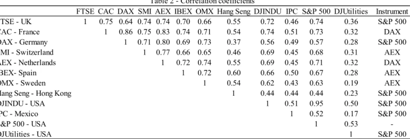
In order to find the best instrument, we build a correlation matrix between the eleven indexes analysed, with the addition of the S&P 500. Table 2 reports the results of this procedure.
As a main criterion, the instrument chosen is the one with the highest correlation coefficient, since a higher correlation coefficient will generally provide better estimates. Still, due to mismatches between the periods of data available for each index, it is possible that the index with the highest correlation is not selected as instrument. In this case, the instrument is the index Table 2. Correlation coefficients – Reported are the correlation coefficients between each index computed for the analysis relative to the Instrumental Variables estimation. The last column of the table reports the instrument chosen for each index. Note that the instrument chosen might not be the index with the highest correlation coefficient if this choice would result in a significant decrease in the number of observations available. Instead, the instrument corresponds to the index with the highest correlation coefficient that allows for the smallest decrease in our data sample.
FTSE CAC DAX SMI AEX IBEX OMX Hang Seng DJINDU IPC S&P 500 DJUtilities Instrument FTSE - UK 1 0.75 0.64 0.74 0.74 0.70 0.66 0.55 0.72 0.46 0.74 0.36 S&P 500 CAC - France 1 0.86 0.75 0.83 0.74 0.71 0.54 0.74 0.51 0.73 0.32 DAX DAX - Germany 1 0.71 0.80 0.69 0.73 0.37 0.56 0.49 0.57 0.28 S&P 500 SMI - Switzerland 1 0.77 0.66 0.65 0.46 0.69 0.45 0.68 0.31 AEX AEX - Netherlands 1 0.72 0.74 0.55 0.69 0.45 0.71 0.32 DAX
IBEX- Spain 1 0.72 0.60 0.66 0.50 0.67 0.28 AEX
OMX - Sweden 1 0.54 0.62 0.43 0.63 0.19 AEX
Hang Seng - Hong Kong 1 0.44 0.44 0.44 0.23 S&P 500
DJINDU - USA 1 0.51 0.95 0.50 S&P 500
IPC - Mexico 1 0.52 0.17 S&P 500
S&P 500 - USA 1 0.53
-DJUtilities - USA 1 S&P 500
9 with a correlation that is among the highest, and that allows for the smallest loss in the number of observations. Taking this into account, an index may be used as an instrument more than once or not at all.
For most cases, this difference in the correlation is not very high. For example, by choosing the S&P 500 as an instrument for FTSE instead of CAC, the loss is less than 2 percentage points. Nonetheless, there are also cases where much larger decreases were necessary in order to avoid losing a very significant amount of observations. This is the case of DAX, where S&P 500 is also chosen as instrument, with a coefficient of 0.57, while the highest correlation coefficient belonged to CAC with 0.86. This change prevents a loss of over 200 observations in a total of nearly 500, a very significant percentage.
Only 3 of the 12 indexes are used as instruments, with S&P 500 being used 5 times. However, it is worth noting that, as concluded by Bartholdy and Peare (2005), “there are large differences in estimated betas depending on the index” chosen for estimation. With this in mind, it is reasonable to assume that, by using different instruments, the results of our estimations will be different. Assume, for example, that we chose Dow Jones Utilities as an instrument for all our estimations. Since it shows the lowest correlation coefficients amongst all indexes, the error resulting from the estimated market returns would be much larger, and our estimations would be less efficient. This is the reason behind choosing instruments with a correlation among the highest.
The previously mentioned authors also show that an equal-weighted index, like CRSP or Dow Jones, can yield better results than a value-weighted index. However, the approach taken by the authors disregards the level of correlation between a stock and the market it is listed in, given that this proxy for the market portfolio generally has the highest correlation coefficient with the stock and is able to explain a higher percentage of the stock’s returns. Still, by using a different index, other than the one where the stock is listed, they also manage to avoid possible endogeneity problems, even though that is not the focus of their assignment. By estimating betas using different estimation methods to eliminate endogeneity, we are able to evaluate if our procedure can produce good results, and, at the same time, compare our results with the ones of the previously mentioned authors.
10 After selecting the appropriate instrument, we estimate the following equation for the IV method using OLS:
𝑟𝑀,𝑡= 𝛾0,𝑡+ 𝛾1,𝑡∗ 𝑟𝑖𝑛𝑠𝑡𝑟𝑢𝑚𝑒𝑛𝑡,𝑡+ 𝜀𝑡 (2) This equation is estimated using five years of monthly data and using a rolling window approach, similar to the estimation of the regular model. The result of this estimation consists on a vector for alpha and beta, with a dimension of (n-59x2), for each market. Regarding the 2SLS, the process is identical, except that eleven instruments are used instead of one. We decide to use all of the instruments to include as much information as possible in our estimations. Using this many instruments can create several problems. One of them is multicollinearity, which will affect the estimated coefficients in this auxiliary regression. A possible improvement to this procedure consists in computing a Sargan-Hansen statistic to test the validity of the instruments, and, in case some of them are not valid, removing them from the estimation process. This should reduce multicollinearity problems by removing insignificant variables from the estimation, and therefore increase the accuracy of our estimations. This is something that is taken into account when analysing the results. Since IV only requires one instrument in the estimation process, only the best one is chosen, and problems like the one described above are not a concern.
By running equation (2) for all the periods of each index we obtain, for each index, a vector of expected returns of the index. A particular detail is that, in the case of IV, the size of this output depends on the number of observations available for each index. However, in the case of 2SLS, the output for all indexes is based on the same time frame, since we are restricted by the index with the least amount of data. These estimates for the market returns are then used as input in the initial model, in place of the true return of the market, which is regressed using OLS, as shown by equation
𝑟𝑖,𝑡 = 𝛼𝑖,𝑡+ 𝛽𝑖,𝑡∗ 𝑟̂ + 𝜀𝑀,𝑡 𝑡 (3) After completing all the estimations for the three methods, we obtain, for each company, three vectors of betas (and alphas) corresponding to each estimation method. These values are the core of all the analysis of the results, which are mostly focused on efficiency gains.
One drawback of these estimation methods is the loss in the number of observations. Since we need to estimate the return of a particular index – using the observations from t=1 to t=60 – we can only estimate the first beta using (1) from t=60 to t=119, meaning that 59 observations are
11 “lost”. In addition, due to discrepancies between the available data across indexes and instruments, the loss of observations may be larger and vary between estimations. In particular, the loss in observations for each index when using IV is around 59, but to estimate using 2SLS, as mentioned before, since we use every index in the sample, we are restricted by the index with the least number of observations - SMI. Therefore, the estimations for 2SLS occur in the period from May 1998 to December 2014. Another problem related to these estimation procedures consists in finding good instruments, since this choice is not entirely dependent of quantitative processes. One possible approach could be trying numerous instruments and using the ones that provide the best results. Unfortunately, that process is considered data mining, since we are analysing which instrument would fit the data in the best way possible, instead of starting from a logical theoretical point of view which would then be applicable to other samples as well.
3.2. Analysing the estimates
We now move on to the processes used regarding the analysis of our results. To evaluate the efficiency of our estimations, we begin by examining our in-sample results, specifically, by computing the average alpha for the entire sample period. This is done for each index, for all the indexes combined, and for the three estimation methods. Next, the percentage of positive and negative alphas is analysed, both at an index level and by pooling all the companies together. Again, the process is repeated for the three estimation methods. These first two steps are taken to check if there are outliers in our sample, but, most importantly, to check for major mistakes in our calculations. We should expect that alpha averages out to zero, and that the distribution of the alphas is slightly biased towards positive alphas.
After this, we check the percentage of companies, in each index, for which the average alpha for the entire sample is significant at a 5% level. This is also an important analysis since, according to the CAPM theory, alpha should be zero. If a method can estimate alphas that are statistically zero a higher percentage of times, then it is likely that the method is able to better fit the data and to represent reality in a more correct way. Considering that we expect to eliminate endogeneity effects, making our estimations more efficient, IV and 2SLS should have less companies with significant alphas. In addition, we run a test to assess whether the difference between the proportions of significant alphas of the three methods is statistically
12 significant. The first step consists on computing a pooled proportion by using the following formula
𝑃𝑜𝑜𝑙𝑒𝑑 𝑃𝑟𝑜𝑝𝑜𝑟𝑡𝑖𝑜𝑛1,2 =(𝑝1∗𝑛1+𝑝2∗𝑛2)
(𝑛1+𝑛2) (4)
where p1 is the proportion of significant alphas in sample 1 and n1 is the size of sample 1. The same reasoning follows for p2 and n2. Secondly, we use the next formula to compute the standard error
𝑆𝑡𝑎𝑛𝑑𝑎𝑟𝑑 𝐸𝑟𝑟𝑜𝑟 = √𝑃𝑃 ∗ (1 − 𝑃𝑃) ∗ (1
𝑛1+
1
𝑛2) (5)
with PP corresponding to the Pooled Proportion calculated in the previous step. Finally, a Z-score is computed using the next equation
𝑍 − 𝑆𝑐𝑜𝑟𝑒1,2 =𝑝1−𝑝2
𝑆𝐸 (6)
where Z follows a normal distribution. The test is performed for all three scenarios – OLS vs IV, OLS vs 2SLS, and IV vs 2SLS.
As a next step, we compare the average R-squared of each index across estimation methods. Here, the reasoning is quite opposite to the general knowledge regarding R-squared. If IV and 2SLS are able to eliminate endogeneity effects, then the R-squared obtained by these estimation methods should be smaller. This should happen because, according to our hypothesis, we assume that the model suffers from endogeneity problems. If this is valid, the independent variable influences the dependent one. The dependent variable then affects the independent one. This circular effects tends to overestimate R-squared.
Lastly, we run an exercise based on the Mean Squared Error (MSE) of the in-sample estimations of the three methods. Starting with an index, for each company, we use the output of equation (1) in order to compute the expected return given by the model. Then, this expected return is compared with the true return by computing a squared error, which assesses the accuracy of the estimation.
𝑆𝑞𝑢𝑎𝑟𝑒𝑑 𝐸𝑟𝑟𝑜𝑟 = (𝑟𝑖,𝑡− 𝐸(𝑟𝑖,𝑡))2 (7) This process is then repeated for every stock in the sample, and for every period available. By averaging all the squared errors, we obtain the MSE of that particular index. The result of this
13 procedure consists of three MSE for each index, relative to each one of the estimation methods. Additionally, another measure is calculated to evaluate possible efficiency gains. This measure can be related with the Goyal Welch R-squared introduced by Welch and Goyal (2008). We apply the formula, supplied by Welch and Goyal (2008), with a few changes
𝐸𝑓𝑓𝑖𝑐𝑖𝑒𝑛𝑐𝑦 𝐺𝑎𝑖𝑛𝑠 = 1 −𝑀𝑆𝐸1
𝑀𝑆𝐸2 (8)
The subscripts 1 and 2 are related with the estimation methods we are comparing(2). In their
paper, Welch and Goyal try to find equity premium predictors that are able to consistently beat the historical average, by comparing the mean squared error of the supposed predictor with the mean squared error of the historical average. Since our study is focused on the three estimation methods, we replace the historical average and the predictors with the results of our methods. Finally, we develop an out-of-sample analysis very similar to the approach taken by Bartholdy and Peare (2005). For each index, and for each time period (month), we run the following cross-section regression using every stock available in the sample:
𝑟𝑖,𝑡+1 = 𝛼𝑖,𝑡+1+ 𝜆 ∗ 𝛽𝑖,𝑡+ 𝜀𝑖,𝑡+1 (9)
In this regression, β is actually the regressor, and 𝜆 is the coefficient to be estimated, which corresponds to the market return of the following period. The objective of this analysis is to see whether the beta calculated in one period can significantly predict the market return (or risk premium in case of raw returns) of the following period. It is important to highlight that the significance of this parameter is essential for the model to be valid. We also look at the
R-squaredof the regression to assess how much of the returns of the following period can be
predicted by beta.
In our analysis across estimation methods, we compare the average R-squared, and the percentage of times that the model is able to predict the market return significantly. Since this factor is of critical importance for the model to be valid, instead of just comparing these percentages across methods, we decide to run the test composed of equations (4), (5) and (6). The results allow us to conclude if there are significant differences between the methods relative to their predictive accuracy.
Lastly, we look at the values for the average R-squared when the predicted market return is positive and significant. This last measure is not presented by the authors but is, in our opinion, (2) Consider, for example, that the result is 0.05. Then, by using method 1 to compute the returns of a company, the mean squared error would be 5% smaller.
14 important to include, especially to make comparisons between the IV and 2SLS, since we expect that they are able to predict market returns more often. This exercise is done at an index level but also for all the indexes together. The main expectation is that both IV and 2SLS outperform OLS in most of these indicators and indexes, since the estimations using these methods ought to be more efficient according to our main hypothesis. However, we also consider the possibility that these methods yield worse results as we increase the size of the index, considering that as the size of the index increases, the effects of endogeneity tend to disappear as companies become atomistic.
4. Empirical Analysis
This section is divided in two parts. In the first part, we analyse the results of our in-sample estimations. After that, we provide more details regarding the out-of-sample analysis.
4.1. In-sample results
Table 3.1 and 3.2 provide statistics regarding the alpha parameter obtained from equation (1) for the three estimation methods.
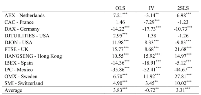
Table 3.1 - In-sample alphas: mean
OLS IV 2SLS AEX - Netherlands 7.21*** -3.14** -6.98*** CAC - France 1.46 -7.29*** -1.23 DAX - Germany -14.22*** -17.73*** -10.73*** DJTUILITIES - USA 2.95*** 1.38 -1.26 DJON - USA 11.98*** 8.33*** -9.83*** FTSE - UK 15.77*** 8.68*** 21.68***
HANGSENG - Hong Kong 10.55*** 15.92*** 14.97***
IBEX - Spain -14.36*** -18.91*** -5.12***
IPC - Mexico -35.86*** -52.41*** -44.67***
OMX - Sweden 6.70*** 11.92*** 27.81***
SMI - Switzerland 4.90*** 3.45** 10.02***
Average 3.83*** -0.72** 3.31***
Table 3.1. In-sample alphas: mean – Reported are the results of the alpha parameter obtained from equation (1), ri,t= αi,t+
βi,t∗ rM,t+ εi,t, for the 11 indexes in our sample, and for the three estimation methods tested. The stars next to each value
correspond to the level of significance - *** at a 1% level, ** at a 5% level, and * at a 10% level. In addition, the last row of the table reports the average value for the alpha statistic obtained by pooling all the companies of the 11 indexes together. All the values are presented in basis points.
15 The objective of this analysis is to assess the presence of outliers and possible mistakes in our calculations. According to CAPM theory, the alpha in the market should average out to zero. The values of alpha for each index display a wide range, from -52.41 b.p. to 27.81 b.p. However, when we look at the average of the entire sample, which would theoretically be closer to the market portfolio, alpha is closer to 0, registering 3.83 basis points for OLS, significant at a 1% level. IV and 2SLS register smaller values for the average alpha. Particularly, IV shows a value of -0.72 basis points, with a t-stat of -1.98, which is not significant at a 1% level and barely significant at a 5% level. We would like to point out the values obtained for Dow Jones Utilities, the smallest index in the sample, for which the gains in efficiency should be more evident. In this case, alpha goes from 2.95 basis points when using OLS, to statistically 0 for IV and 2SLS. As expected, IPC and Hang Seng, the outliers in our sample, report the most extreme values for alpha, with values ranging from -52.41b.p. to 15.92b.p.
Despite 2SLS and IV reporting lower values for the average alpha, there is no clear pattern regarding index size. Since alpha is still significant for almost all estimations, we decide to undergo another test. Table 3.2 reports the result of this analysis, where we evaluate the percentage of positive and negative alphas, both at an index level, and by averaging all the indexes together.
The expected result of this exercise is a slight bias towards the positive alphas, and that is exactly what we find. For OLS and IV, 9 out of the 11 indexes report this bias, whereas 2SLS
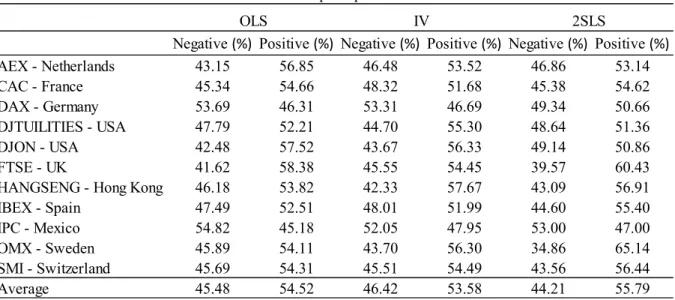
Negative (%) Positive (%) Negative (%) Positive (%) Negative (%) Positive (%)
AEX - Netherlands 43.15 56.85 46.48 53.52 46.86 53.14 CAC - France 45.34 54.66 48.32 51.68 45.38 54.62 DAX - Germany 53.69 46.31 53.31 46.69 49.34 50.66 DJTUILITIES - USA 47.79 52.21 44.70 55.30 48.64 51.36 DJON - USA 42.48 57.52 43.67 56.33 49.14 50.86 FTSE - UK 41.62 58.38 45.55 54.45 39.57 60.43
HANGSENG - Hong Kong 46.18 53.82 42.33 57.67 43.09 56.91
IBEX - Spain 47.49 52.51 48.01 51.99 44.60 55.40 IPC - Mexico 54.82 45.18 52.05 47.95 53.00 47.00 OMX - Sweden 45.89 54.11 43.70 56.30 34.86 65.14 SMI - Switzerland 45.69 54.31 45.51 54.49 43.56 56.44 Average 45.48 54.52 46.42 53.58 44.21 55.79 IV OLS 2SLS
Table 3.2 - In-sample alphas: distribution
Table 3.2. In-sample alphas: distribution – Reported are the percentages of positive and negative alphas resulting from equation (1), ri,t= αi,t+ βi,t∗ rM,t+ εi,t, for the 11 indexes in our sample, and for the three estimation methods tested. The last row
reports the average values for the indicators obtained by pooling all indexes together. All the values are presented in percentage points.
16 reports 10 indexes with more positive than negative alphas. The average values for this parameter, for all estimation methods, are very close, ranging from 53.58% to 55.79%.
The results of these two tests allow us to continue with our analysis, knowing that there are should be no major mistakes in our calculations. However, some improvements could be made. More specifically, since we are using a rolling window approach, each estimation will be composed of 59 observations that are included in the previous estimation, and only 1 new observation. This can create problems related with autocorrelation that will affect the standard deviations of our parameters.
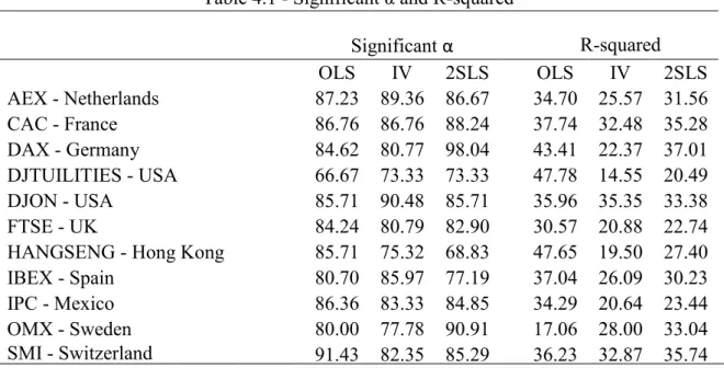
Table 4.1 - Significant α and R-squared
Significant α R-squared OLS IV 2SLS OLS IV 2SLS AEX - Netherlands 87.23 89.36 86.67 34.70 25.57 31.56 CAC - France 86.76 86.76 88.24 37.74 32.48 35.28 DAX - Germany 84.62 80.77 98.04 43.41 22.37 37.01 DJTUILITIES - USA 66.67 73.33 73.33 47.78 14.55 20.49 DJON - USA 85.71 90.48 85.71 35.96 35.35 33.38 FTSE - UK 84.24 80.79 82.90 30.57 20.88 22.74
HANGSENG - Hong Kong 85.71 75.32 68.83 47.65 19.50 27.40
IBEX - Spain 80.70 85.97 77.19 37.04 26.09 30.23
IPC - Mexico 86.36 83.33 84.85 34.29 20.64 23.44
OMX - Sweden 80.00 77.78 90.91 17.06 28.00 33.04
SMI - Switzerland 91.43 82.35 85.29 36.23 32.87 35.74
Table 4.1 is divided in two main components. The first three columns correspond to the percentage of companies in each index for which the average value of the alpha estimated is significantly different from 0 at a 5% significance level. According to CAPM theory, the alpha in the regression should be zero in order to avoid any arbitrage opportunities. Despite the fact that this does not apply entirely to the real world, by checking if the constant is significant a lower amount of times, we can evaluate if beta is more able to explain the dependent variable. This is in fact linked to the other statistic provided in the table, the average R-squared of the Table 4.1 Significant alpha and R-squared – The first three columns present the percentage of companies for which the output of equation (1) reported alphas significant at a 5% level. This analysis is displayed for all the 11 indexes as well as for the 3 estimation methods. The last three columns show the average value of the R-squared for all the companies in each index. The values for both measures are presented in percentage points.
17 regressions for the entire index. Generally speaking, the higher the R-squared, the better the model fits the data.
As expected, given our previous analysis, the amount of alphas that are significant is very high. Nonetheless, we still run this analysis to see if there are significant differences between estimation methods. By looking at the table, we can see that for only 1 out of the 11 indexes – Dow Jones Utilities – does OLS show the smallest percentage of significant alphas. For all the other indexes, there is at least one of the other two methods that outperforms OLS in this measure. Moreover, in 4 indexes – FTSE, Hang Seng, IPC, and SMI – both IV and 2SLS manage to get lower percentages of significant alphas than the OLS. Additionally, the average value of this measure is higher for OLS than for the other two estimation methods, despite the lack of a pattern when analysing the results index by index. To see whether this difference is significant, we run a test to evaluate differences in proportions, using equations (4), (5) and (6), reported in Table 4.2.
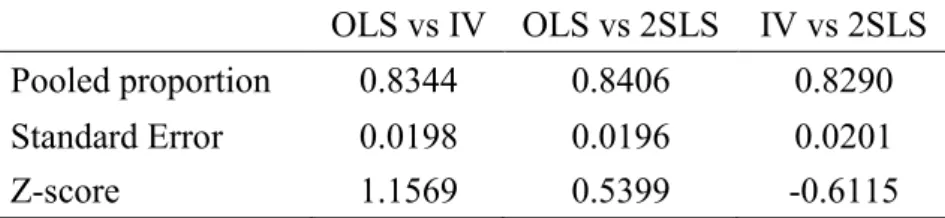
Table 4.2 - Testing difference in proportions
OLS vs IV OLS vs 2SLS IV vs 2SLS
Pooled proportion 0.8344 0.8406 0.8290
Standard Error 0.0198 0.0196 0.0201
Z-score 1.1569 0.5399 -0.6115
By looking at the Z-scores of the test, we can see that the difference in proportions of significant alphas regarding the three estimation methods is not significant. This result is expected since, when analysing table 4.1, we are unable to see a clear pattern regarding index size or estimation method. We are therefore unable to conclude anything regarding efficiency gains at this point.
Moving back to Table 4.1, and analysing the results relative to the R-squaredobtained, the
results are practically opposite. For all but one index in the sample – OMX – OLS reports values that are higher than the other two estimation methods. The conclusion then seems to be that OLS is the model that is most able to explain the returns of the companies. However, we should expect a higher R-squared for the regressions that use OLS, since these regressions are still affected by endogeneity. With endogenous regressors, the regressor affects the dependent Table 4.2. Testing difference in proportions – Reported are the results of equations (4), (5) and (6), relative to the pooled proportion, the standard error, and the Z-score of the test. Both the pooled proportion and the standard error values are reported in percentage points.
18 variable, which in turn affects the regressor, and so on. This “circular” behaviour is bound to overestimate the percentage of the variation of the dependent variable that is explained by the regressor. Therefore, the R-squared that they report is not actually accurate.
Overall, these results are still not very conclusive. The differences in alphas are not significant, and we are still unable to conclude if the lower values for R-squared are indeed due to the elimination of the endogeneity effects, or simply because the model is a worse fit for the data. We need to continue with the additional tests before we can make more general conclusions. Table 5 reports the results regarding the analysis of the MSE obtained through equations (7) and (8).
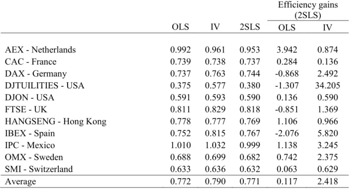
Table 5 - Mean Squared Error
Efficiency gains (2SLS) OLS IV 2SLS OLS IV AEX - Netherlands 0.992 0.961 0.953 3.942 0.874 CAC - France 0.739 0.738 0.737 0.284 0.136 DAX - Germany 0.737 0.763 0.744 -0.868 2.492 DJTUILITIES - USA 0.375 0.577 0.380 -1.307 34.205 DJON - USA 0.591 0.593 0.590 0.136 0.590 FTSE - UK 0.811 0.829 0.818 -0.851 1.369
HANGSENG - Hong Kong 0.778 0.777 0.769 1.106 0.966
IBEX - Spain 0.752 0.815 0.767 -2.076 5.820
IPC - Mexico 1.010 1.032 0.999 1.138 3.245
OMX - Sweden 0.688 0.699 0.682 0.742 2.375
SMI - Switzerland 0.633 0.636 0.632 0.063 0.629
Average 0.772 0.790 0.771 0.117 2.418
In the first three columns of the table, we can see the monthly mean squared errors, in percentage points. These are the average estimation errors occurred in when estimating the expected return using the CAPM, regardless of the estimation method. Several conclusions can be drawn from this table. First, 2SLS is the method that reports the lower average MSE, 0.771%, immediately followed by OLS, with 0.772%. IV reports the highest values for this measure, 0.790%, not only on average, but also for the majority of the indexes tested. In fact, its MSE is Table 5. Mean Squared Error – Reported are the results relative to equation (7), 𝑆𝐸 = (𝑟𝑖,𝑡− 𝐸(𝑟𝑖,𝑡))2,regarding the calculation
of the Mean Squared Error. Also, in the last two columns, we report the values for the efficiency gains calculated, using as benchmark the performance of the 2SLS estimates. The last row of the table reports the average values for the measures obtained by pooling all the companies and indexes together. All the values are presented in percentage points.
19 the biggest in 8 of the 11 markets, and is never the lowest among the three estimation methods. Secondly, 2SLS outperforms OLS in 7 of the 11 markets, but, similarly to the analysis of the significance in alphas, there is not a consistent pattern, regarding, for example, the index size. Additionally, the difference in the average MSE for all the indexes is extremely low - close to 0.001%. A value this small may not be sufficiently large to overcome the estimation errors in out-of-sample performance.
We also report, in the last two columns of the table, the results of equation (8). The values correspond to the efficiency gains relative to using 2SLS instead of the other two estimation methods. The interpretation is that, for instance, by using the estimates of beta provided by 2SLS to estimate the returns of a company in AEX, as opposed to OLS, the estimation error is reduced by 3.942% on a monthly basis. The conclusions are in accordance with the first part of the table. By estimating with 2SLS instead of IV, taking into account all the indexes, our monthly MSE is reduced by 2.418%, a very significant amount if we extrapolate this result to an annual equivalent. Alternatively, by replacing our OLS estimates with 2SLS, the monthly decrease in our error is only 0.117%, which is expected given the extremely small difference in the average MSE of these two methods.
These in-sample analyses suggest a difference between the results of IV and 2SLS, with the latter yielding the most efficient estimates. However, the differences between OLS and 2SLS results are still not significant nor strong enough to justify the use of 2SLS as opposed to the simpler OLS. We must test the performance of these methods in an out-of-sample analysis to evaluate whether these markets can, in fact, benefit from more complex estimation methods, when taking into account estimation error.
4.2. Out-of-sample results
It is very common for complex models to work well in-sample, but be outperformed by more simplistic models in an out-of-sample analysis, since the efficiency gains are usually not sufficient to overcome the estimation error. DeMiguel, Garlappi and Uppal (2009) test 14 models regarding asset allocation in several datasets and conclude that no model is able to consistently beat the naive diversification of 1/n. Taking this into account, and considering our in-sample results are not very conclusive, we decide to perform an out-of-sample analysis to
20 assess if 2SLS and IV are able to capture efficiency gains that can overcome the estimation errors.
To do this, we follow a procedure similar to Bartholdy and Peare (2005) as shown by equation (9). Table 6 reports the results of this exercise.
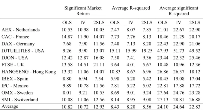
Table 6.1 - Out-of-Sample results
Significant Market Return Average R-squared Average significant R-squared
OLS IV 2SLS OLS IV 2SLS OLS IV 2SLS
AEX - Netherlands 10.53 10.98 10.05 7.47 8.07 7.85 21.01 22.67 22.90 CAC - France 14.87 11.90 14.07 7.73 7.76 8.13 18.46 21.29 20.17 DAX - Germany 7.68 7.90 11.56 7.40 7.13 8.20 22.43 22.90 21.06 DJTUILITIES - USA 9.26 9.90 13.07 15.11 15.99 19.25 47.93 51.73 49.52 DJON - USA 12.42 12.87 16.08 7.50 7.41 9.36 23.44 22.32 25.46 FTSE - UK 13.58 14.51 21.11 3.64 4.01 5.67 10.48 10.96 12.36 HANGSENG - Hong Kong 13.32 11.06 14.07 10.83 8.67 6.96 26.86 26.37 18.12 IBEX - Spain 8.80 6.94 7.54 5.98 5.28 5.42 18.45 19.08 17.04 IPC - Mexico 9.89 10.78 11.56 7.81 5.22 5.02 22.81 17.88 17.72 OMX - Sweden 8.01 9.21 10.55 8.69 9.01 9.24 27.64 24.76 23.28 SMI - Switzerland 10.08 11.06 12.56 8.14 8.95 9.08 27.13 28.81 26.88 Average 10.82 10.72 12.93 8.43 8.20 8.56 24.10 24.64 22.83
The objective of this analysis is to evaluate the predictive power of beta. More specifically, we are interested in assessing whether beta can significantly predict the return of the market, and if this predictive power is influenced by the method through which we estimate beta. In
addition, we also look at the R-squaredof the regression to see how much of the next period’s
returns can be predicted by the beta calculated in the previous month. Note that, if beta is unable to estimate the market return significantly, the evaluation of the R-squared is negligible, since according to Bartholdy and Peare (2005), “significance of this value is a necessary condition for the model to be of any use”. Because of this, we find it logical to begin our analysis by looking at the percentage in significance of the market return, the first three columns of the table.
Table 6.1. Out-of-sample results – Reported are three statistics relative to the output of equation (9),𝑟𝑖,𝑡+1= 𝛼𝑖,𝑡+1+ 𝜆 ∗ 𝛽𝑖,𝑡+
𝜀𝑖,𝑡+1. The first three columns provide, for each index and for each estimation method, the percentage of periods for which the
estimate of the market return of the following period, obtained from equation (9), is positive and significant at a 5% level. The middle three columns report the average value of the R-squared for the entire sample period. The last three columns report the average of the R-squared only for the periods in which the market return estimated is positive and significant at a 5% level. The last row reports average values for the three indicators obtained by pooling the results of all the indexes together instead of analysing them one by one. All the values in the table are reported in percentage points.
21 The percentage of times OLS is able to predict the return of the market significantly is only higher for 2 indexes – CAC and IBEX. For all the other indexes, there is at least one estimation method that outperforms OLS considering this measure. In fact, in 7 of the remaining indexes, both IV and 2SLS are able to significantly predict the market return more times than OLS. This result implies that the betas obtained by estimating through IV or 2SLS can predict future market returns more often than the standard OLS betas. If we look at the average values for the entire sample though, only 2SLS is able to outperform OLS, with an accuracy of 12.93%. An important conclusion to retain is that each of the alternative estimation methods proposed outperformed OLS in 8 of the 11 indexes tested. Once again, as a particular detail, we would like to point out the results of the estimations for Dow Jones Utilities. By using 2SLS to estimate the market return, the predictability of beta increases by 3.81 percentage points, which is equivalent to an increase of over 40%. This is one of the best improvements of the entire sample, which can be justified by the size of the index that allows for more efficiency gains obtained by eliminating endogeneity effects.
To evaluate if the differences between the percentages shown by the three estimation methods are significant, we run a difference in proportions test, similarly to the one presented Table 4.2. The results are shown in Table 6.2.
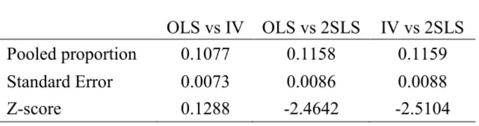
Table 6.2 - Testing differences in proportions
OLS vs IV OLS vs 2SLS IV vs 2SLS
Pooled proportion 0.1077 0.1158 0.1159
Standard Error 0.0073 0.0086 0.0088
Z-score 0.1288 -2.4642 -2.5104
The Table reports the values for the pooled proportions and standard errors required to compute the Z-score relative to the test. By looking at the results, we can see that the difference between the percentage of times 2SLS is able to predict the market return, relative to both OLS and IV, is significant at a 5% level. This result supports our previous conclusion which states that estimates obtained with 2SLS are able to more frequently predict market returns significantly. Additionally, we also conclude that there is no statistical difference between IV and OLS in Table 6.2. Testing difference in proportions – Reported are the results of equations (4), (5) and (6), relative to the pooled proportion, the standard error, and the Z-score of the test. Both the pooled proportion and the standard error values are reported in percentage points
22 terms of this measure. This result is in line with our previous tests, given the fact that IV and OLS reported very similar values on this measure, 10.72% and 10.82%, respectively, and that IV is the model that reported less efficiency gains in our in-sample estimations.
Focusing now on the middle three columns of the Table 6.1, related to the average R-squared of the model, the conclusions are similar. 2SLS is again the only model to beat OLS, in 8 out of the 11 indexes, despite the difference being smaller, with an average value of 8.56%. This demonstrates a higher predictive power of the returns that follow the estimation period. These two results – lower percentage of significant market returns and a lower R-squared – suggest a poorer out-of-sample performance of OLS, related with 2SLS, which can be explained by the known inconsistency of OLS. Amano, Kato and Taniguchi (2012) find that, in the presence of long-memory dependence between the error term and the independent variable, OLS estimates become inconsistent, and their suggestion is also the use of 2SLS. Similarly to the previous indicator, we also compare the results by index. The results are similar, with OLS scoring a higher R-squared in only 3 of the 11 indexes – HangSeng, IBEX and IPC. This model is then outperformed in the remaining of the indexes, reporting the lowest value among the three estimation methods for 6 indexes. The results concerning the IV estimator remain weaker. In addition to reporting a similar percentage in the predictability of market returns, it is outperformed by OLS in the R-squared measure in 5 of the 11 indexes and, in fact, exhibits a lower average than OLS.
Like in previous analyses, if we consider an approach index by index, we are unable to detect any sort of pattern regarding index size. Also, the difference in the average value of the R-squared is not large, only 0.13% when considering OLS and 2SLS.
By combining the results obtained when analysing the market return and the R-squared, we conclude that the three estimation methods are able to predict similar percentages of the return of the stock. However, 2SLS is the model that is able to make these predictions more frequently, thus being the most efficient estimator in our sample.
Finally, the last three columns of Table 6.1 relate to the average R-squared of the regression when the market return is positive and significant at a 5% level. Once again, OLS underperforms to at least 1 of the other methods in 8 of the 11 indexes. However, when we look at the average values in this case, IV is the method that outperforms OLS, instead of 2SLS. In fact, 2SLS performed poorly on this analysis, given that it only displays higher values than OLS in 5 indexes. One possible reason for 2SLS to perform worse in this measure, compared with
23 the other ones where it seemed to always surpass IV, is that the model may contain too many variables. Some of the instruments may not be good enough to be included in the estimation process, and therefore they might be decreasing the performance of the model in both this test and all the other measures evaluated. A further improvement could then consist on computing the test mentioned in the methodology section – Sargan-Hansen statistic – to enhance the model and remove any unnecessary instruments. Considering that 2SLS already seems to be the best model amongst the three, any improvements in the estimation process would only support this conclusion.
Summing up, the conclusions of this exercise are the following. First, the betas estimated through 2SLS are able to predict the market return a higher percentage of times than OLS and IV. Secondly, the estimates provided by 2SLS also manage to better forecast the returns of the period that follows the estimation of beta. The results seem to indicate that 2SLS might be the model that delivers the most robust results and is therefore better to use when estimating beta. This is based on the fact that IV only delivered better results in 1 index on the significance of the market return, and on 2 indexes in the R-squared approach. A possible explanation for this could be that 2SLS uses a lot more information on its estimation than IV, given that it includes 11 instruments in the process of estimating the endogenous variable. This model is therefore closer to the reality of financial markets. For example, the recent crash of the Chinese stock market had a huge negative impact both in European and American stock markets. By including information such as this in our estimations, we believe that the coefficients estimated should be closer to the real ones.
Additionally, since 2SLS is able to outperform OLS in the out-of-sample analysis, we can conclude that the decrease in the R-squared in the in-sample estimations is, in fact, due to the elimination of the endogeneity effects, and that the returns of other markets are a good instrument, considering that they were able to generate efficiency gains.
5. Conclusion
In this thesis, we investigate the hypothesis of endogeneity in the CAPM. More specifically, we analyse 11 markets that should be more susceptible to endogeneity effects due to their size. We find evidence of these effects by comparing the estimates obtained through OLS with two models that estimate efficiently in the presence of endogenous regressors, IV and 2SLS. The
24 results obtained demonstrate that estimates obtained through 2SLS can significantly predict market returns more often than the regular OLS estimates. Moreover, the R-squared on this analysis is also higher for 2SLS, for the majority of the indexes analysed. This means that not only is 2SLS able to predict market returns with more frequency, but the percentage of future returns that it is able to predict is also higher. 2SLS is the model that provides the most efficient results. However, the IV estimates, in most of the measures analysed, prove unable to beat the OLS estimates.
By using the formulations proposed throughout this thesis, the estimation errors incurred in when opting for these more complex estimation methods are small enough to justify their estimation instead of OLS. This is translated by the gains in efficiency we obtain by eliminating or reducing the endogeneity effects and finding a consistent estimator. Considering the major importance of estimating consistently in financial markets, whether the sensitivity of an asset to the variation of a market or the expected return of a given company, we recommend replacing the traditional OLS CAPM with 2SLS to any investor or manager working in these markets or one with similar conditions, since it should improve their predictive power and accuracy. As a topic for further research, we suggest adjusting the performance of the 2SLS estimator by testing the adequacy of all the instruments used. Given that it already outperformed the other two estimators, possible improvements coming from this adjustment would only enhance this result. Additionally, we propose replicating the analysis of this thesis in bigger markets, to test at what point the hypothesis of atomicity of companies starts to be true, and the endogeneity effects become insignificant.
6. References
Amano, Kato and Taniguchi (2012). Statistical Estimation for CAPM with Long-Memory Dependence. Advances in Decision Sciences, 1-12.
Bartholdy and Peare (2003). Unbiased estimation of expected return using CAPM. International Review of Financial Analysis, 12, 69-81.
Bartholdy and Peare (2005). Estimation of expected return: CAPM vs Fama and French. International Review of Financial Analysis, 14, 407-427.
25 Bruner, Eades, Harris, Higgins (1998). Best practices in estimating the cost of capital: survey and synthesis. Financial Practice and Education, 13-28.
Carhart (1997). On Persistence in Mutual Fund Performance. The Journal of Finance, 52, 57-82.
DeMiguel, Garlappi and Uppal (2009). Optimal Versus Naïve Diversification: How Inefficient is the 1/N Portfolio Strategy? The Review of Financial Studies, 22 no.5, 1915-1953
Fama and French (1993). Common Risk Factors in the Returns on Stocks and Bonds. Journal of Financial Economics, 33, 3-56.
Hahn and Hausman (2003). IV Estimation with Valid and Invalid Instruments. MIT Working Paper.
Lai and Stohs (2015). Yes, CAPM is dead. International Journal of Business, 20(2), 144-158. Lintner (1965). The Valuation of Risk Assets and the Selection of Risky Investments in Stock Portfolios and Capital Budgets. The Review of Economics and Statistics, 47, 13-37.
MacKinlay (1995). Multifactor models do not explain deviations from the CAPM. Journal of Financial Economics, 38, 3-28.
Mossin (1966). Equilibrium in a Capital Asset Market. Econometrica, 34, 768-783.
Sharpe (1964). Capital Asset Prices: a Theory of Market Equilibrium under Conditions of Risk. The Journal of Finance, 19, 425-442.
Somerville and O’Connell (2002). On the Endogeneity of the Mean-Variance Efficient Frontier. The Journal of Economic Education, 33:4, 357-366.
Welch and Goyal (2008). A Comprehensive Look at the Empirical Performance of Equity Premium Prediction. The Review of Financial Studies, v 21 n 4, 1455-1508