0 NEW UNIVERSITY OF LISBON
Faculty of Science and Technology
Integrated Masters Degree in Electrical Engineering and Computers
SEGMENTATION OF STRIATAL BRAIN STRUCTURES FROM HIGH RESOLUTION PET IMAGES
by
Ricardo Jorge Pires Correia Farinha
Dissertation presented at the Faculty of Science and Technology of the New University of Lisbon in fulfillment of the requirements for the Masters degree in Electrical Engineering and Computers
Supervisors: Prof. José Manuel Fonseca Prof. Ulla Ruotsalainen
Lisbon 2008
1
Preface
This thesis was carried out during the 2007-08 academic year in the Methods and Models for Biological Signals and Images (M2oBSI) research group, at the Institute of Signal Processing, Tampere University of Technology, Finland.
First, I want to express my deepest gratitude to my parents and family for all the support and encouraging given during my studies. Without them none of this would be possible.
I want to thank my supervisors, Professor Ulla Ruotsalainen (TUT), Professor José Fonseca (FCT-UNL) and senior researcher Jussi Tohka, PhD (TUT) for this opportunity, for their guidance, and for all the support given to me during the elaboration of this thesis.
I thank senior researcher André Ribeiro, PhD. for the patience to read through the thesis and pointing out many useful improvements.
I thank to all my colleagues in M2oBSI research group for always finding time to help and advise me when needed. I specially thank to Antonietta Pepe and Uygar Tuna, my office colleagues, for all the help and friendship.
I wish to thank to Marika Kovanen, in particular, and all my friends for their endless help and encouragement whenever needed.
Lastly, I would like to thank the collaborators in Turku PET Center, University of Turku/Turku University Central Hospital for the outstanding collaboration, for providing useful information on the physical principles behind HRRT scanners and for providing the PET data.
Tampere, May 2008. Ricardo Farinha Kärkikuja 2C 76 33720 Tampere, FINLAND +358 44 94 54 397 [email protected]
2
Abstract
We propose and evaluate fully automatic segmentation methods for the extraction of striatal brain surfaces (caudate, putamen, ventral striatum and white matter), from high resolution positron emission tomography (PET) images. In the preprocessing steps, both the right and the left striata were segmented from the high resolution PET images. This segmentation was achieved by delineating the brain surface, finding the plane that maximizes the reflective symmetry of the brain (mid-sagittal plane) and, finally, extracting the right and left striata from both hemisphere images. The delineation of the brain surface and the extraction of the striata were achieved using the DSM-OS (Surface Minimization – Outer Surface) algorithm. The segmentation of striatal brain surfaces from the striatal images can be separated into two sub-processes: the construction of a graph (named “voxel affinity matrix”) and the graph clustering. The voxel affinity matrix was built using a set of image features that accurately informs the clustering method on the relationship between image voxels. The features defining the similarity of pairwise voxels were spatial connectivity, intensity values, and Euclidean distances. The clustering process is treated as a graph partition problem using two methods, a spectral (multiway normalized cuts) and a non-spectral (weighted kernel k-means). The normalized cuts algorithm relies on the computation of the graph eigenvalues to partition the graph into connected regions. However, this method fails when applied to high resolution PET images due to the high computational requirements arising from the image size. On the other hand, the weighted kernel k-means classifies iteratively, with the aid of the image features, a given data set into a predefined number of clusters. The weighted kernel k-means and the normalized cuts algorithm are mathematically similar. After finding the optimal initial parameters for the weighted kernel k-means for this type of images, no further tuning is necessary for subsequent images. Our results showed that the putamen and ventral striatum were accurately segmented, while the caudate and white matter appeared to be merged in the same cluster. The putamen was divided in anterior and posterior areas. All the experiments resulted in the same type of segmentation, validating the reproducibility of our results.
3
Table of contents
1. Introduction …...6
2. Human striatal neuroanatomy ……….…………...…….11
2.1. Striatum ...11
2.2. Dorsal striatum ………...…12
2.2.1. Caudate nucleus ………..…12
2.2.2. Putamen ……….……..…...12
2.3. Ventral striatum………...………...13
3. Positron Emission Tomography (PET) ………...…...….15
3.1. Tracer technology ………...………...16
3.2. Distribution of the intensity values in a PET image ………..………..17
3.3. ECAT HRRT PET scanner ………...18
4. Deformable models ………...19
4.1. Medical Image Analysis using Deformable Models ………...20
4.2. Deformable Curves………....21
4.3. Deformable Surfaces ………...23
4.3.1. DSM (Dual Surface Minimization) algorithm ………...…….……….23
4.3.2. DSM-OS (Dual Surface Minimization-Outer Surface) algorithm ………...…25
4.4. Incorporating “A priori” knowledge ………...26
5. Graph-Based Image Segmentation ………..27
5.1. Spectral methods for clustering ……….…..28
5.2. Normalized cuts ………...28
5.3. Non – spectral methods ……….……...31
4
6. Segmentation of striatal structures ……….…….34
6.1. Pre-processing steps ……….……...34
6.2. Segmentation of the striatum into four structures ……….………..36
6.2.1. Affinity matrix construction methods ..……….….…...37
6.2.2. Clustering methods ………...….39 6.3. Implementation ……….………...41 7. Experiments ………...…………..….42 7.1. Material ………....42 7.2. Results ……….………43 7.2.1. Phantoms ………...………..43 7.2.2. Real HRRT images ……….………..47
8. Discussion and conclusion ……….…...51
References ………53
Appendix 1: Eigenvectors and Eigenvalues ……….……….…59
Appendix 2: Segmentation results ………..……...60
Appendix 3: Putamen subdivision ………...64
5
Abbreviations
AP – Anterior putamen BGO – Bismuth germinate BP – Binding potential CD – Caudate
CT – Computer tomography DOI – Depth-of-interaction DSM – Dual surface minimization
DSM-OS – Dual surface minimization - outer surface
FCT-UNL – Faculty of Science and Technology-New University of Lisbon (Portugal) FDG – Fluorodeoxyglucose
FMRI – Functional magnetic resonance imaging FOV– Field of view
H – Hydrogen
HRRT – High resolution research tomograph IC – Internal capsule
LSO – Lutetium orthosilicate LV – Left ventricle
MRI – Magnetic resonance imaging N – Nitrogen
NCUT – Normalized cut O – Oxygen
OP-OSEM-3D – Ordinary poisson-ordered subsets expectation maximization in full 3D PET – Positron emission tomography
PP – Posterior putamen ROI – Region of interest
TUT – Tampere University of Technology (Finland) 2D – Two dimensional
6
1. Introduction
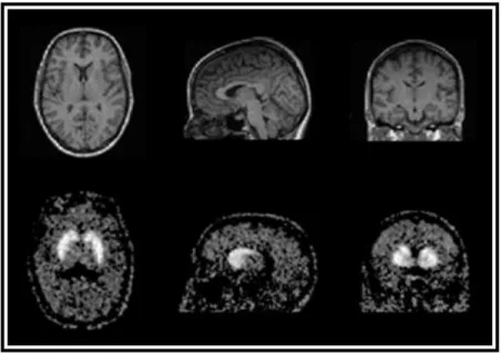
The development and proliferation of medical imaging technologies is revolutionizing medicine [1]. Medical imaging can extract clinical information on anatomic structures through computed tomography (CT), magnetic resonance imaging (MRI). Medical imaging also allows obtaining functional information using positron emission tomography (PET), and others, with almost no harmful effects to the body and noninvasively. Besides visualization of anatomic structures, medical imaging is now also used to do surgical planning and simulation, intra-operative navigation, radiotherapy planning, and to track the progress of diseases [1]. E.g., radiotherapy can subject a tumor to a specific dose of radiation with minimal collateral damage to healthy tissue. Each imaging modality was developed to provide information on particular aspects of the imaged object. X-ray based computed tomography (CT) produces images based on the photon attenuation as the X-rays goes through the tissue. Magnetic resonance imaging (MRI) imaging measures the proton or water density. MRI and CT images are used to visualize the anatomical structure of the subject, since they allow distinguishing between different tissues. Positron emission tomography, presented in more detail in chapter 3, and functional MRI imaging (fMRI) inform on the functional properties of the tissue. In figure 1.1 are shown cross-sections acquired with MRI and PET.
Figure 1.1. Examples of medical images from the head, transaxial,sagittal and coronal views. (top) A T1-weighted MRI image, (bottom) PET image. The images are from diferent subjects. The images were provided by Turku PET Center.
7
Although modern imaging devices attain high quality anatomical views, the analysis of the image data via computational methods is still very limited, and requires human intervention. The development of more advanced computational methods will allow extracting and interpreting quantitative data efficiently and in a repeatable way, which can then be used to support a wide range of tasks, from diagnosis to clinical interventions.
One aspect in which computational methods can contribute is in image segmentation. For this to be possible, it is necessary to accurately determine the boundaries of each structure. This has been shown to be unattainable by traditional low-level image processing techniques since they only account for local information, giving rise to incorrect assumptions during the integration process, which leads to generating unrealistic object boundaries.
Most clinical segmentation is currently done by manual slice editing, that is, a human operator manually delineates the region of interest on each 2D slice of the 3D image. This process has several disadvantages, for example, the results will be dependent on any bias of the operator, when viewing each 2D slice and deducing the spatial shape of 3D structures. Also relevant to the results is the fatigue of the operator, due to the enormous amount of data that must be manually or semi-automatically extracted. This makes the process expensive, if feasible, and, more importantly, the final result might not be easily reproducible by another operator, hampering the comparability between the segmentation results.
Automation of medical image analysis is a highly complex, not only due to the complexity of the shapes one wants to extract but also due to the variability within and across individuals. The noise in medical images results from a complex combination of noise from several sources, e.g. measurement noise, natural intensity variation within structures of interest, and modality dependent imaging artefacts [2]. This makes the task of suppressing noise and artificially correcting its effects a difficult task. Since different imaging modalities use different measurement devices, they are subject to different sources of noise and differ in noise levels. Importantly, the effects of noise can vary in different structures of interest which causes additional difficulties in their discrimination, since discrimination is done calculating the differences in intensity values rather than intensity values themselves [2].
The aim of this thesis is to improve and extend the methods presented in [3]. There, the authors proposed an automatic method to extract striatal structures, namely, caudate and putamen, from binding potential PET images. The data acquisition was done using the (ECAT EXACT HR+, Siemens CTI, Knoxville, TN) scanner and on the dedicated GE Advance PET scanner (GE Medical Systems, Waukesha, WI). The methodology in [3] can be divided in the following steps: 1. Extract the brain surface using a deformable model.
2. Extract hemisphere images from the extracted brain surface. 1. INTRODUCTION
8
3. Extract the left and right striatum from the left and right hemisphere images using a deformable model.
4. Extract putamen and caudate from both right and left striata.
The deformable models have been used to segment, visualize, track, and quantify a variety of anatomical structures (see chapter 4 for a more detailed description) and a general overview on deformable models. The methods used to extract the information from the images in steps one to three are explained in chapters 4 and 6. The extraction of the putamen and the caudate in step four is done using a 2-way normalized cut algorithm [3]. In chapter 5 is presented an overview on the Graph-Based image segmentation, and more specifically, on the normalized cuts algorithm. The development of the new brain-dedicated, high-resolution PET scanner (ECAT HRRT, Siemens Medical Solutions, Knoxville, TN) that provides images with enhanced resolution, step four in [3] fails to segment the striatal structures. The lack of success was due to the excessive computational complexity of the segmentation algorithm. This excessive computational complexity became prohibitive due to the enhancement of the resolution of the new HRRT scanner. This resolution enhancement allows distinguishing more than two structures in the PET data. Therefore, the method used in [3] to extract the striatal structures (2-way normalized cut algorithm) became obsolete since it can only manage the separation into two structures. In this study, we aim to overcome this limitation and develop an algorithm capable of separating the striatum into four structures (caudate, putamen, ventral striatum, and white matter). Due to the limited success of the previous method, this thesis proposes the use of a mathematically identical method, but that is able to dwell with the increased complexity of the new type of high resolution images.
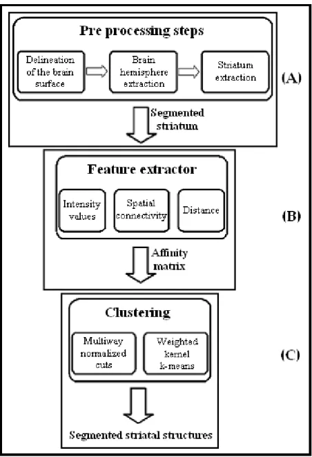
In short, this thesis presents new automatic techniques to successfully extract striatal brain structures, namely putamen, caudate, and ventral striatum, from PET HRRT binding potential images. In chapter 2, information is given about the structures that the proposed method aims to extract. The automatic method consists of a series of consecutive steps shown in the hierarchy graph below (figure 1.2).
9
Figure 1.2 Steps of the segmentation of caudate, putamen, ventral striatum. (A) Preprocessing steps, (B) affinity matrix construction method, (C) clustering process.
The preprocessing step (figure 1.2 (A)) consists on the extraction of the striatum, from HRRT PET binding potential images. This extraction method is the same as the one used in [3] and is described above. However, some tuning of the initial parameters was necessary.
Once the striatum was extracted, several features of the striatal voxels are computed (figure 1.2 (B)). This information is then stored in an affinity matrix and provided to the clustering algorithm. The image features used are Euclidean distances between voxels, spatial connectivity and intensity values. The affinity matrix contains the similarity values between all pairs of voxels. That is, in position i, j is written the similarity value between voxels i and j, thus, this 1. INTRODUCTION
Intensity values
10
matrix is symmetric and all values in the diagonal are equal to 1, see section “affinity matrix construction methods” for the methodology and an example. Determining the affinity matrix is a crucial step to guarantee enough smoothness so that the clustering process can provide a good segmentation.
Finally, the clustering algorithm segments the image (figure 1.2 (C)). The clustering procedure is treated in this thesis as a graph partition problem. Two approaches were developed that are capable of partitioning the graph: the multiway normalized cuts and the weighted kernel k-means. In both methods, the affinity matrix represents the graph that one wants to partition into different regions. The strategy used in the multiway normalized cut algorithm is to apply the k-means clustering algorithm to the computed graph eigenvalues in order to partition the image into connected regions. On the other hand, the weighted kernel k-means classifies, iteratively, each voxel as belonging to a cluster. This classification is done using the information contained in the affinity matrix (graph) of the image. Although this procedure allows successively extracting the desired structures of interest, it has some subtleties. Namely, a careful initialization is required in each step, to obtain maximum accuracy, i.e., the final result depends on the number of desired clusters, initial estimative for the clustering result, maximum distances and spatial connectivity allowed between voxels and, number of iterations. These parameters have to be carefully tuned to provide the most accurate result. The same values were found to be the optimal for all tested HRRT PET image, thus no further tuning was required. Chapters 6 and 7 give, respectively, a detailed description of the methodology and results. In chapter 8, the discussion and conclusions of the results are presented.
11
2. Human striatal neuroanatomy
The aim of this thesis is to develop efficient automated methods to extract striatal brain structures from high resolution PET images. To this aim, in this chapter, the structures of interest are introduced.
The brain is the center of the human nervous system and the main regulator of the ongoing processes in the human body. The human brain is composed of white and gray matter and is surrounded by three layers of special soft tissue. The white matter is the area of the brain whose nerve fibers are involved in myelin responsible for the coloration [4]. The gray matter consists mainly of nerve cell bodies (neurons). Its gray brown color is due to the neuronal capillary blood vessels and the neuronal cell bodies [4].
The human brain is centrally divided into two hemispheres that are connected by bridges of white matter. The brain structure is usually characterized by dividing it six lobes, depending on the function to which they have been associated to. Four lobes are visible from the outside, namely, the frontal, the parietal, the occipital and, the temporal lobe, while the other two are internal: the insula and limbic lobes. The frontal lobe is mainly associated with reasoning, planning, parts of speech, movement, emotions, and problem solving. The parietal lobe is associated with movement, orientation, recognition, perception of stimuli. The occipital lobe is associated to visual processing and the temporal lobe is associated to perception and recognition of auditory stimuli, memory, and speech [5].
2.1. Striatum
The striatum is an individual entity with a toric topology. There is one striatum in each brain hemisphere. The striatum is composed by several structures (figure 2.2): the caudate, the putamen and the ventral striatum. The caudate is the closest to the center of the brain, the putamen the furthest away and the ventral striatum is beneath them. The putamen and caudate are separated by the anterior limb of the internal capsule [5], however there are some bridges of white matter connecting these structures. These structures are all contiguous, making difficult the delimitation of the ventral striatum. A debate is still ongoing within the medical community to delimitate its boundaries.
The striatum is best known for its role in the planning and modulation of movement pathways but is also involved in a variety of other cognitive processes involving executive functions. In humans, the striatum is activated by stimuli associated with reward, but also by aversive, novel, unexpected or intense stimuli [5].
12
2.2 Dorsal striatum
2.2.1. Caudate nucleus
The caudate nucleus has an arched geometry that can be separated into two main structures, namely, the head and the tail also referred to as the body of the caudate. The head is located in the anterior portion of the caudate and it is an enlarged area when compared to the tail. The head of the caudate nucleus and the putamen are horizontally separated with a tract of white matter and, the bottom of each of these structures is vertically connected by the nucleus accumbens. The tail is connected to the head of the caudate and it elongates circularly, passing through the back of the brain. The tail forms the roof of the inferior horn of the lateral ventricle.
Recently, it was demonstrated that the caudate is highly involved in learning and memory, particularly regarding feedback processing [6]. It is known that neural activity occurs, in general, in the caudate while an individual is receiving feedback. The left caudate has been suggested to be related with the thalamus, which governs the comprehension and articulation of words as they are translated between different languages [7].
2.2.2. Putamen
The putamen is the largest striatal structure. This structure is cytologically uniform, but is not uniform in terms of the functional behavior of its components. The putamen complex is divided into discrete striosomes, embedded in a background matrix, the extrastriosomal matrix [5]. The matrix and striosome have several chemical differences, e.g. if the putamen is stained immunocytochemically with enkephalin one can observe that this compound will be concentrated in the areas where the striosomes are, which is around the striosomes periphery [8]. The putamen has various types of connections and neurotransmitters. It receives most of its inputs from the motor and somatosensory areas of the cortex. The putamen outputs are delivered mainly to the globus pallidus and thalamus. This information will then be delivered to the motor, premotor and supplementary motor areas. Therefore, the putamen is considered to be a major player in most of the striatal motor functions [5].
The putamen can be divided into two sub regions, the anterior and posterior putamen (figure 2.1), as defined respectively as ventral and dorsal putamen [9]. The anterior putamen is composed by gray matter which is bounded by the anterior and posterior limbs of the internal capsule, and, laterally, is bounded by the external capsule in the first three planes ventral to the plane containing the dorsum of the putamen. The posterior putamen is bounded by the pallidum, by an external capsule, and by the internal capsule [9].
13
Figure 2.1 Striatum subdivisions, (CD) caudate, (AP) anterior putamen, (PP) posterior putamen. The image is from [10].
2. 3. Ventral striatum
In the literature, the striatum is usually divided into two areas, the ventral striatum and the dorsal striatum [11]. The dorsal striatum is the sensorimotor-related part of the striatum and it is composed by the putamen-caudate complex. The ventral striatum is related with emotional and motivational aspects of behavior [12]. Dysfunctions of the ventral striatum have been associated among individuals with schizophrenia [13], obsessive-compulsive disorder [13], depression, and drug addiction [14].
So far, no structural or functional marker has been identified that allows an accurate distinction between ventral and dorsal striatum. Commonly, this separation is assumed to be between the caudate-putamen complex and the core and shell structures of the nucleus accumbens (figure 2.2). However, the ventral striatum is not composed only by the nucleus accumbens, but it extends ventrally through the caudate and putamen [11], [15].
The nucleus accumbens is divided into two areas (shell and core structures) according to their specific function [16]. The shell is the structure located at the lower bottom of the nucleus accumbens (figure 2.2). The shell is known to be involved in the expression of certain innate, unconditioned behaviors, such as feeding and defensive behavior [17]. The core is located above the shell and it is responsible for response-reinforcement learning. The shell and core subregions play important but distinct roles in instrumental conditioned learning that may be potentiated with psychostimulants [16].
14
In short, the ventral striatum, a specific region of the striatum, is the structure responsible for connecting the limbic, cognitive, and motor systems within the striatum. Experimental studies in animals have shown that the ventral striatum plays an important role in several forms of behavioral learning [18].
Figure 2.2 Right striatum, Core and Shell belonging to the nucleus accumbens we can consider the nucleus accumbens as the ventral striatum, Put (putamen) and Caud (caudate), IC (internal capsule). The image is from [18].
15
3. Positron Emission Tomography (PET)
Positron Emission Tomography (PET) is the medical imaging technology used to acquire the images to which the proposed methods are applied. In this chapter a theoretical introduction to its principles is given.
Positron emission tomography (PET) is a widely used medical imaging technology. Within the several categories of medical images, PET is categorized as a functional imaging modality. This means that PET imaging devices have the ability to observe physiological functions in vivo, and from these create three dimensional dynamic models. This functional information provides the enhancement of the understanding that the medical community has of the biochemical basis of normal and abnormal bodily functions [19]. PET can be used to explore the functioning of the internal organs of both animals and humans.
PET imaging integrates two technologies: the tracer kinetic assay method and computed tomography (CT). The tracer kinetic assay method consists of introducing a radio labeled biologically active compound (tracer) into the subject blood flow, and in using a mathematical model to describe the kinetics of the tracer as it participates in a biological process. The tracer kinetic model requires information about the tissue tracer concentration, measured by the PET scanner [20].
During PET acquisition, one administrates into the patient, by injection or inhalation, a positron-emitting compound containing a radioactive isotope. This compound will concentrate in specific regions of the body, with a given (unknown) density. When one emitted positron encounters an electron, they annihilate each other and produce two photons of 511 keV. The photons will move in opposite (180°) directions, to conserve momentum. The energy of these photons is usually sufficient to allow the photons to “escape” the subject body, being then detected by the detector rings that surround the subject (figure 3.1 (B)).
For an emission event to be counted, both photons must be registered nearly simultaneously (within a time window τ) at two opposite detectors (scintillation crystals composed of e.g. bismuth germanate (BGO)), i.e. they must occur on the same coincidence line (figure 3.1 (A)) [19]. The absolute value of the counts in a PET scan results from the counts of true coincidences plus the counts of random coincidences. True coincidences are coincident events that originate from a single annihilation process, while random coincidence events occur when, accidentally, a pair of detectors located in opposite positions record an uncorrelated signal within a time window τ.
The detectors of the PET scanner are arranged in cylindrical shaped rings. This property allows the scanner to register the events in three dimensions. From this set of data, the spatial
16
distribution of the radioactivity in the body can be reconstructed by using appropriate reconstruction algorithms [21]. All measured coincidence events (valid events detected by a pairs of detectors) are stored into sinograms. A sinogram is a two–dimensional matrix where the columns store each image projection angle and the rows store the spatial positions within the (measured) projections, i.e. they are projection views at different angles [22]. The reconstruction algorithms take into account all the coincidence events stored in the sinogram, at all angular and linear positions, when reconstructing the image.
The image quality in PET is strictly related with the applied image reconstruction method. The positron emission data acquisition is not free from noise, namely, there is a substantial amount of statistical noise that arises from the statistical nature of the decay of the positron emitted by radio-labeled isotope [23].
Figure 3.1. (A) [18F] annihilation and the positron emission tomography (PET) coincidence principle, (B) interior of the HRRT scanner chamber. The images are from [21] and (from presentations of J. Johansson).
3.1. Tracer technology
The tracer technology is one of the fundamental keys in PET imaging. The main idea behind this technology is that before the compound is injected into the subject’s blood flow, an artificial isotope has to replace an atom of the compound. This isotope is a radio-labeled tracer artificially engineered that, when injected in the blood flow, can be detected from outside the body. The 3. POSITRON EMISSION TOMOGRAPHY (PET)
17
tracer does not change the chemical properties of the compound, ensuring that the biochemical process to be studied is not altered.
The atoms that are usually artificially replaced by their isotopic forms are carbon (C), hydrogen (H), nitrogen (N), and/or oxygen (O). These stable molecules are replaced respectively by C, N11 13 or O 15 . These radiolabeled isotopes, whose decay results is the emission of a
positron, are ideal for this purpose due to their short half-life, respectively (11C half-life is 20 min; 13N, is 10 min; O15 , is 2 min) [21]. However, their short life expectancy requires their production to be quickly followed by their introduction in the patient, a difficult and rigorous task. For this reason, the production of these compounds by the cyclotron is usually performed near the place of application into the patient.
Raclopride labeled with 11C is used as a PET tracer to study the function of dopaminergic synapses. Raclopride binds to dopamine D2 receptors and is a selective, reversible inhibitor of dopaminergic D2 receptor function [20].
The radiation generated by the injected compound is absorbed by the subject tissue according to its mass. This absorption can be quantified by the PET scanner or by computer tomography (CT). The resulting dynamic data can be collected from specific biological structures (regions of interest) by recording its radioactivity over time [21]. This recording is done in predefined time frames in which the analyzed targets are scanned.
To analyze the results from the scans, one needs an estimation of how the tracer binds to the region of interest receptors. This information is stored in the so called parametric binding potential (BP) images. By definition, the binding potential is a measure of the ratio of concentration of specific binding and is a reference concentration at equilibrium [24]. These images are obtained from the recorded dynamic data, through the use of a predefined model, e.g., the “simplified reference tissue model” [25].
3.2. Distribution of the intensity values in a PET image
The spatial distribution of intensity values within an image depends on the radiopharmaceutical applied [23], that is, on the uptake areas defined by the tracer. The uptake area of a receptor-like tracers is the one with the highest concentration of the tracer type receptors. For example, if the tracer used is 11C raclopride, the higher uptakes will be found in the striatal area because it is the region with the highest densities of dopamine D2 receptors in the human brain, and therefore it will have the highest intensity values. In short, image volumes with higher intensity values than its surroundings are classified as the functional region for the applied tracer [23].
18
3.3. ECAT HRRT PET scanner
The ECAT HRRT (High Resolution Research Tomograph) is a dedicated 3D-only brain scanner. This tomography device is imbued with the new LSO scintillators. It uses depth of interaction (DOI) information to achieve uniform isotropic resolution across a 20cm diameter volume [26]. In Positron Emission Tomography there is a continuous effort to increase the sensitivity and to improve spatial resolution up to its physical limits. For high sensitivity a compact geometry is needed. Also good spatial resolution requires a small diameter of the detector arrangement to reduce the effect of the angular deviation from 180 degrees of the two annihilation photons. A compact geometry entails an increase in scatter and random coincidences. Random rates can be reduced by a shorter coincidence window, which requires a fast crystal. The other prerequisite for improved resolution is a reduction in crystal size, which necessitates a crystal material with high luminosity. If good resolution shall be preserved over a large volume in a scanner with a compact geometry and a small crystal size, depth of interaction (DOI) needs to be measured additionally. The High Resolution Research Tomograph scanner was designed to meet all these challenges. It employs the new scintillator LSO (Lutetium Oxy Orthosilicate). Its high light yield allows a reduction in crystal size and its short scintillation rise and decay time a short coincidence time window and a reduction of the dead time.
The single crystal layer in HRRT scanner consists of eight flat panel detector heads, arranged in an octagon. The distance between two opposing heads equals 46,9cm. Each head contains 9x13 LSO crystal blocks of 7.5mm thickness, which are cut into 8x8 crystals, resulting in 7488 individual crystal elements per head and 59 904 crystals for the entire gantry. The size of one crystal equals 2.1x2.1x7.5mm. The HRRT scanner has a 31.2cm transaxial and 25.5cm axial FOV and a gantry port diameter of 35cm.
In [3], one of the scanners used for the acquisition was the Exat Ecat HR+. This scanner was running in 3D mode during acquisition. From the scan, 13 frames were obtained, with dimensions of 128x128x63 slices and voxel size of 2.11x2.11x2.11 mm3. In comparison, the HRRT scanner
extracted images whose size is 200x200x150 slices with an isotropic voxel dimension of 1.22x1.22x1.22 mm3, making the automatic analysis of this data a more defying task when using
the HRRT scanner due to the size of the images to extract. 3. POSITRON EMISSION TOMOGRAPHY (PET)
19
4. Deformable models
In this chapter an overview is presented on deformable models. These models are used in the striatum extraction from the high resolution images.
The development of digital imaging technologies made possible the use of automated techniques of imaging processing, which have an increasingly crucial role in medical imaging. Image segmentation is now used at a daily base in medical environment. There are many different applications for image segmentation, e.g. quantification of tissue volumes, diagnosis, localization of pathology, study of anatomical structures, treatment planning, and computer-integrated surgery [27].
There is no standard approach to a segmentation problem. The adequate segmentation procedure varies according to the data and the application in use. One possible definition for image segmentation is: “Image segmentation refers to a process of dividing the image data into regions whose voxels have some common property such as uniform gray-level. A region is a group of voxels with similar properties. Regions often correspond to or have a link to objects” [28].
The characteristics of the data and the inexistence of a method to assess the validity of the result of the segmentation requires the use different segmentation algorithms. As a consequence, new segmentation problems require experimental validation of the segmentation algorithms used for that particular problem. Moreover, image segmentation is not yet an easy task in terms of computational complexity. Although the increasing computation power continuously improves the state of the art, several problems remain whose solution is still very challenging, namely, removal of intrinsic noise of the images, removal of image artifacts, improvements of image resolution, etc. These problems arise due to the object shape and image quality variability and the limited resolution allowed by the scanners. Therefore, when applying classical segmentation techniques, for example, edge detection or “thresholding”, they have a high probability of failure. When using these classical techniques, one has to apply sophisticated image preprocessing or postprocessing techniques to obtain good segmentation results, decreasing the failure rate [27].
The most popular image segmentation methods used for intensity images (image represented by point-wise intensity levels) are: thresholding, edge-based methods, region-based methods, and deformable models. The threshold techniques base their decisions on local voxel information and are suitable to segment objects that fall outside the range of intensity levels of the background. Spatial information is ignored in these methods, decreasing their robustness. Some examples of the application of these methods can be found in [29], [30]. The edge-based methods were developed to detect contours. These methods are “fragile” when the images have broken contour lines. Moreover, their robustness is also highly reduced if there are blurred regions. Some
20
examples can be found in [31]. Region-based methods rely on grouping neighboring voxels of similar intensity levels to segment the image, thus, the image is partitioned into connected regions e.g. [32]. Deformable models usually start with some given boundary shape formed by spline curves, and iteratively modifies its topology by applying various shrink/expansion operations according to a predefined energy function e.g. [3; 33]. There is a risk that the computation of the energy minimization becomes trapped in some local minimum of the energy function. Fortunately, optimization algorithms can be added that solve this problem.
Deformable models are a successful approach to image analysis, by combining geometry, physics, and approximation theory concepts, and have proven to be effective in segmenting, matching, and tracking anatomic structures, being capable of coping with the diversity of biological structures [1].
Deformable models can be subdivided into two subcategories, deformable curves and deformable surfaces, respectively, to solve two dimensional or three dimensional image segmentation problems. These curves or surfaces are defined inside the image plane or volume, and will be deformed until the desired segmentation result is reached. To obtain the deformations, internal and external forces are applied. The internal forces are defined within the curve or surface and are designed to smooth the model during deformation. The external forces depend on the image data and are applied to move the curve or surface toward an object boundary or other desired features within an image.
By introducing a priori knowledge about the shape of the object of interest, deformable models become more robust to noise and boundary gaps. This initialization makes deformable models very suitable for being applied in medical imaging, because the human anatomy is well known. Deformable models have a low sensitivity to their initialization, e.g. assumed initial surfaces or curves, initial anatomic information, etc. This quality allows using automatic methods without the need of human intervention, thus making them suitable to analyze large sets of data. On essence, this is an iterative method whose goal is, at each step, to find the global minimization of the surface energy function [23].
4.1. Medical Image Analysis using Deformable Models
Deformable models were first developed for computer vision and computer graphics problems. However, their potential when applied to medical image analysis was soon discovered. Deformable models show increased accuracy, precision, reproducibility when compared with the limited manual slice editing and traditional image processing techniques. These models can be used in a variety of medical imaging technologies such as X-ray, computed tomography (CT), angiography, magnetic resonance imaging (MRI), ultrasound and, PET. Deformable models have 4. DEFORMABLE MODELS
21
been used to segment, visualize, track and quantify a variety of anatomical structures. These include the brain, heart, face, cerebral, coronary and retinal arteries, kidney, lungs, stomach, liver, skull, vertebra, brain tumors, fetus, and even cellular structures such as neurons and chromosomes [1].
Deformable models consider the object boundaries as a whole and can make use of “a priori” information about the object shape to aid in the segmentation problem. The inherent continuity and smoothness of the models can compensate for noise, gaps and other irregularities in object boundaries. Furthermore, the parametric representations of the models provide a compact, analytical description of object shape. These properties make this technique robust and elegant in linking sparse or noisy local image features into a coherent and consistent representation of the object.
4.2. Deformable curves
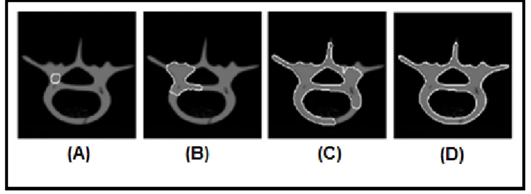
The first deformable models were used to segment two dimensional structures. One of the first of these deformable models to be used was snakes [34] (figure 4.1). These algorithms are usually initialized by the user. A deformable contour (figure 4.1 (C)) is first defined. Next, this contour expands until it reaches the boundaries of the region of interest (figure 4.1 (d), (e), (f)). The final result of the segmentation procedure can still be tuned by the user. This tuning is done by changing the models parameters until a smoother segmentation result is obtained. The final segmentation consists in a single two dimensional slice that can be used as a first guess in neighbouring image slices, sparing the user the burden of initializing manually the contour of each image slice. If there is a sequence of two dimensional image scans, one can analyze them individually. After segmenting all the image slices, the information accumulated can then be aggregated into a continuous three dimensional surface model.
Figure 4.1. (A) Intensity CT image of LV. (B) Edge detected image. (C) Initial snake. (D)-(F) Snake deforming towards LV boundary, driven by “inflation” force . The images are from [33]. 4. DEFORMABLE MODELS
22
However, these two dimensional segmentation approaches have some limitations. As mentioned, they are designed to be interactive methods; however in most medical applications it is necessary to initialize the contours automatically near the regions of interest limiting their applicability. Another limitation is that the objective function, used to allow these methods to expand automatically, can constrain their geometric flexibility and prevent the curves/contours from representing long tube-like shapes or shapes with significant protrusions or bifurcations (figure 4.2) [1]. Classic methods are topology dependent, i.e. they are parametric models and one must provide in advance topological information about the structure of interest.
Figure 4.2 Image sequence of clipped angiogram of retina showing automatically subdividing snake flowing and branching along a vessel. The images are from [33].
Due to these limitations, more advanced methods that can automatically cope with topological changes were developed. These shape modelling schemes, topology independent, can be deformable contours or deformable surface models. They can extract long tube-like shapes or shapes with bifurcations (figure 4.2), and also sense changes in the topology (figure 4.3).
Figure 4.3. Segmentation of a cross sectional image of a human vertebra phantom using a topology-adaptable snake. The snake begins as a single closed curve and becomes three closed curves. The images are from [33].
23
4.3. Deformable surfaces
Segmenting 3D image volumes slice by slice, both manually or applying 2D contour models, is a laborious process and requires a post-processing step to connect the sequence of 2D contours into a continuous surface [35]. There are several problems associated with the use of this technique. The most important one arises due to the lack of contextual slice-to-slice information, when analyzing sequences of adjacent 2D images. This lack of information results in inconsistencies in the reconstructed surfaces, such as the appearance of bands or rings.
However, the use of fully three dimensional deformable models instead of using a set of individual contours is a faster and more robust segmentation technique, whose results do not suffer from lack of contextual information, which ensures smoothness and coherent surfaces between image slices.
4.3.1. DSM (Dual Surface Minimization)
The DSM (Dual Surface Minimization) algorithm is a deformable surface model. This algorithm is initialized with two meshes, respectively, the inner and outer meshes. A mesh is defined as a volume composed by a set of edges and vertexes. The inner mesh is located inside the region that one wants to extract and the outer surfaces are placed outside the regions of interest.
Figure 4.4 HRRT PET Scan, Sagittal, Coronal and Transverse views, image provided by Turku PET Center.
A two dimensional representation of the initial meshes is shown in figure 4.4 as a red outline. The volume that lies inside both initial surfaces (meshes) is called “search volume” and is the area to which the minimization process will be applied to, i.e. where the initial meshes will shrink or expand.
24
This algorithm is an iterative method that in each iterative step calculates the energy of the current mesh. The algorithm strives to minimize the energy, giving as output the surface with lower energy, thus it is a typical energy minimization problem. The energy term on the DSM algorithm is divided in two terms, the external and the internal energies. The external energy depends on the underlying image, and its minimization is achieved by drawing the smallest surface that still contains all the salient features of the image while the internal energy controls the shape of the surface [23].
The global energy of the surface informs us of how well the mesh approximates the surface of interest and it is defined as:
E M =N1 λEN int mi mi1, mi2, mi3 + 1 − λ Eext(mi)
i=1 (1)
In (1), Eint is the internal energy, Eext the external energy, the parameter λ is a regularization
parameter that controls the trade off between the internal and external energies. M is a simplex mesh and its denoted by M = m1, … , mN , where mi ∈ ℝ3 are coordinates of the meshes vertex,
and N is the number of vertexes in the mesh. In a simple mesh each vertex mi has exactly three neighbours, whose coordinates are denoted by mij.
Figure 4.5 Simplex mesh with 320 vertexes. The image is from [23]. The internal energy is defined as:
Eint mi mi1, mi2, mi3 = mi −
1 3 3j=1mij
2
A(M) (2)
In (2), A(M) is the average area of the faces of the mesh M. The normalization using the area is required for scale invariance of the internal energy.
The external energy is defined as: 4. DEFORMABLE MODELS
25
Eext mi = 1 − (IT(mi)) ∇IT(mi)
maxxIT(x) ∇IT(x) (3)
In (3), IT is an intensity image, built from the analyzed binding potential image, by applying a
threshold method. If T is the threshold, all voxels from the binding potential image having a higher value than T, will be replaced by that same threshold value. The voxel with smaller value will maintain the original intensity value. The threshold T is automatically determined for each image based on the expected volume of the striatum [3]. This threshold technique is required to correct the high inhomogeneous intensity values within the striatum caused by the partial volume effect, noise, and other image artifacts. The edge image ∇IT(wi) is a discreate approximation of
the gradient, and it is computed using a 3-D Sobel operator [3].
The external energy defined by eq. 3 is application dependent. Therefore, any new segmentation problem requires finding a suitable equation to express the external energy. Equation 3 is used to extract the striatum surface from brain hemisphere images in [3].
For more information about the DSM algorithm see [2].
4.3.2. DSM-OS (Dual Surface Minimization-Outer Surface)
The DSM-OS algorithm (Dual Surface Minimization – Outer Surface) is a variant of the DSM (Dual Surface Minimization) algorithm. It is also initialized with two surfaces meshes: the inner surface, located inside the brain surface and outer surface, outside the brain surface (figure 4.4). The main difference between these two deformable surface methods is that, in the DSM-OS algorithm, only the outer surface moves towards the region of interest. This is, in some cases, advantageous. For example, when extracting the brain surface from positron emission tomography (PET) images, it is preferable to approach the surface of interest from outside due to noise. Outside the brain volume there is no relevant radioactivity and therefore the noise level is lower in that region. Consequently, it is appropriate to use only one surface mesh when approaching the target surface from the outside. The algorithm optimization cycle terminates when it fulfills a condition, namely, when the outer surface reaches the inner surface. Afterwards, the algorithm remembers the mesh of the lowest energy found, and the mesh used to compute that energy is assigned as the desired segmented structure.
26
4.4. Incorporating “A Priori” Knowledge
In medical images, the general shape, location and, orientation of objects are often known and this knowledge may be incorporated into the deformable model as initial conditions, data constraints, constraints on the model shape parameters or, into the model fitting procedure, increasing the accuracy of the final result. The use of implicit or explicit anatomical knowledge to guide shape recovery is especially important for a robust automatic interpretation of medical images. For automatic interpretation, it is essential to have a model that not only describes the size, shape, location, and orientation of the target object but that also can cope with unexpected variations in these characteristics. Automatic interpretation of medical images spares clinicians from the laborious aspects of their work and still provides increased accuracy, consistency, and reproducibility of the interpretations [1].
27
5. Graph-Based Image Segmentation
This chapter describes principles of graph based image segmentation theory that are later on applied. Two types of graph image segmentation approaches are presented, namely, normalized cuts and weighted kernel k-means. The first is a spectral method and the latest a non-spectral graph based approach.
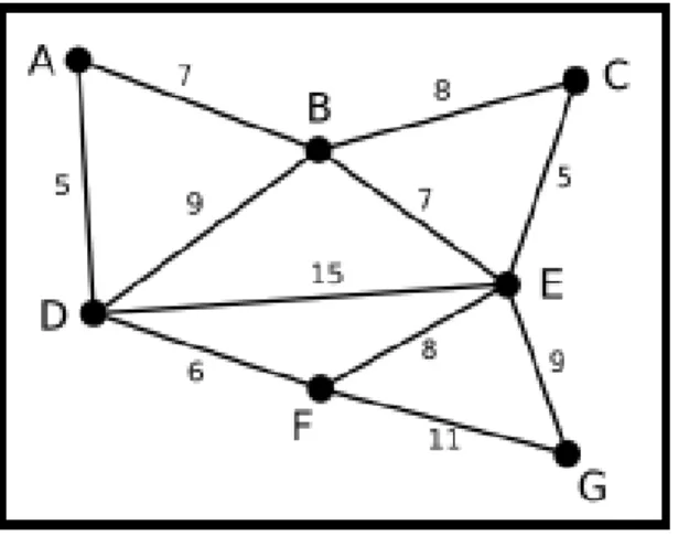
Graph-Based techniques are commonly categorized as region-based image segmentation techniques. To pose image segmentation as a graph partitioning problem, one has to represent how the chosen image features affect the relationship between voxels. This information is represented as weights of the connections between the nodes, i.e., by a weighted graph (figure 5.1) G = N, E with node set N and edge set E [35]. The nodes n ∈ N correspond, for example, to pixels (or voxels) intensity values or position, while the edges connect the nodes ni, nj according to the neighborhood definition in use. Every edge ni, nj ∈ E has a weight. Depending on the problem such weights might represent, for example, costs, lengths or capacities, etc.
Figure 5.1 Weighted graph, where the letters are the set of nodes N, and the numbers the set of edges E.
The constructed image graphs can be directed or undirected. A directed graph is one whose edges are ordered pairs of nodes. In contrast, undirected graphs connect the nodes but the directionality of the connections is not defined. A directed graph may be thought of as a neighborhood of one-way streets. A regular two-one-way street may be thought of as an undirected graph [36].
Minimum spanning trees [37], shortest paths [38] and graph-cuts [39] are some of the used graph algorithms to solve image segmentation problems. Among these methods, graph-cuts is the one
28
that distinguishes itself, due to its computational efficiency and flexibility as a global optimization tool [35].
5.1. Spectral methods for clustering
Spectral clustering methods are region-based image segmentation methods. This approach segments different structures into distinct fragments. One variant of these methods uses the top eigenvectors of a matrix. These eigenvectors are derived from the distance between points. Such methods have been successfully used in many applications including computer vision and VLSI design [39; 40]. However, there are still debates on which eigenvectors to use and how to derive clusters from them.
One method consists in using spectral clustering to partition a spectral graph, such that the second eigenvector of the graph’s Laplacian (matrix representing the image graph, computed by subtracting the degree matrix (D) and the image affinity matrix (A)) is used to define a semi-optimal cut [42]. This method assumes that cuts based on the second eigenvector will attain a good approximation to the optimal graph cut. This analysis can be extended to clustering by building a weighted graph in which nodes correspond to data-points and edges are related to the relative features of the points. Cluster differentiation is done by partitioning the graph, which can be done by a variety of algorithms such as ratio cut [43], Kernighan-Lin Objective [44], and normalized cut [45]. Usually, spectral graph partitioning objectives are used to partition the graph in two. Therefore, when one wants to partition the graph in more than two parts, the partition methods have to be applied recursively to find the k desired clusters. It has experimentally been observed [39; 40] that using more eigenvectors and the direct computation of a k way partitioning improves the results.
5.2. Normalized Cuts
As mentioned above, the normalized cuts algorithm can be used as a criterion to segment a graph. A graph can be partitioned into two disjoint sets by removing the edges connecting the two parts. One can attain the degree of dissimilarity between these two disjoint areas by computing the total weight of the removed edges [42]. This measurement is usually known in graph theory as “cut” and it can be mathematically represented as follows:
cut B, C = u∈B,v∈CA u, v (4) In (4), B and C are two distinct areas, while A u, v is a function of the similarity between nodes u and v, A is also called affinity matrix.
29
To attain the global optimum graph bipartition one has to minimize (4). The number of partitions for a graph with N nodes is 2N. This optimization is a well-studied problem and efficient
algorithms have been developed to solve this problem. However, when there are small sets of isolated nodes in the graph, the minimum cut criteria favors the cut in those areas, even when it is not the optimal cut.
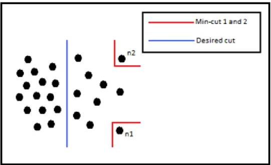
Figure 5.2 Case where the minimum cut criterion fails. The red lines represent the true cuts and the blue line is the ideal cut. The image is from [45].
In figure 5.2 is shown one case where the minimum cut criterion fails, which thereby justifies the need of more sophisticated methods to partition the graph. In this figure it is assumed that the edge weights decrease with the increase of the distance between two nodes. Therefore, when one applies the minimum cut criterion to the image, the nodes n1 and n2will have the minimum cut because they are the ones furthest away from their neighbors. In fact, all the nodes on the right side of the desired cut will have smaller cut value when compared to the nodes to the left.
However, if one uses a method that, instead of relying only on the total edge weight value of the connecting partitions, it also accounts for all connections to all nodes in the graph, the problem described above can be avoided.
This new disassociation measure between two groups, named “normalized cut” (Ncut), was first introduced in [45] and is defined as:
Ncut B, C =assoc (B,V)cut (B,C) +assoc (C,V)cut (C,B) , assoc B, V = u∈B,t∈VA(u, t) (5) 5. GRAPH-BASED IMAGE SEGMENTATION
30
In (5), assoc B, V is the sum of the weights of the connections from nodes belonging to B to all nodes in the graph, and assoc C, V is, similarly, the sum of the weights of the connections from nodes belonging to C to all nodes in the graph [45].
Using this disassociation definition between the groups eliminates the problem that arises when the minimum cut criterion tried to partition small isolated points. Therefore, using the normalized cut criterion to partition small isolated points will, in general, have a large cut value due to the denominators in (5). For example, nodes n1 and n2 from figure 5.2 will no longer have the
smaller cut value, as they did when submitted to the minimum cut criterion. Instead, the Ncut value will increase because the association measure will decrease.
It is shown in [45] that the minimization of the Ncut criterion (5) can be converted into a generalized eigenvalue system:
D − A y = λDy (6) In (6), A represents an affinity matrix and D is an N x N diagonal matrix. The diagonal matrix D is attained by summing each value from each line of the image affinity matrix (A).
D i, i = A(i, j)j (7) The generalized eigenvalue system (6) can be transformed into a standard eigenvalue problem: D−12 D − A D−
1
2x = λx (8)
Solving a standard eigenvalue problem is a difficult task since it requires high computational power. These computations take O n3 operations to compute all the eigenvectors, where n is the
number of nodes in the graph. Therefore when one applies this method to a large image, the number of operations is usually too large, due to the high number of voxels. See appendix 1 for a detailed explanation about eigenvectors and eigenvalues.
We can then partition the graph using the following algorithm [45] which goes through the following the steps:
1. Given an image or image sequence, create a weighted graph with the image information. 2. Solve D − A x = λDx for eigenvectors with the smallest eigenvalues.
3. Use the eigenvector with the second smallest eigenvalue to bipartition the graph.
4. Decide if the current partition should be subdivided and recursively repartition the segmented parts if necessary.
31
In the step one, an affinity matrix is built from chosen image features. Some examples of possible features are spatial connectivity, voxel intensity values, Euclidean distance, etc.
Step two solves (8) to determine the eigenvector of the second smallest eigenvalue. The eigenvalues are the solutions of the normalized cuts mapped from a discrete domain to a continuous domain. Each component in an eigenvector corresponds to a node in the graph. Afterwards, the graph is bipartitioned using the computed eigenvector by thresholding the eigenvector components. The search for the best threshold is done using the Ncut criterion. Only the optimum partition of the eigenvector of the second smallest eigenvalue is searched, because trying to find the optimum partition for all the eigenvectors would not be computationally feasible since there is no algorithm that can solve this problem in “polynomial time”.
Finally, in step four, the algorithm decides if the current partition should be subdivided, considering that the graph is being bipartitioned into more than two clusters. If this assumption holds, the algorithm returns to the initial step and repartitions the sub-graphs found in the first iteration.
There is another way of attaining a k-way partition of the graph that uses more than one eigenvector. If we want to partition the graph in, for example, four partitions, one uses three eigenvectors and each component of each eigenvector will correspond to an image feature. Afterwards, these features are fed to a clustering algorithm e.g., k-means, that will cluster the image based on the given features.
5.3. Non – spectral methods
Spectral clustering, after mapping the original space into an eigenspace, uses the information from the eigenvalues and eigenvectors for graph partitioning. These methods are called spectral, because they make use of the data affinity matrix spectrum to cluster the points. Their efficiency arises from not making any assumptions about the final clusters.
On the other hand, non-spectral methods do not rely on the computation of the eigenvalues and eigenvectors of the image affinity matrix.
5.3.1. Weighted Kernel k-means
The weighted kernel k-means algorithm [46] is a generalization of the standard k-means algorithm [47], and maps points to a higher-dimensional space. Therefore weighted kernel k-means has a major advantage over standard k-k-means, since it can discover clusters that are not linearly separable in the input space.
32
Weighted kernel means was first presented in [48]. It was shown that the weighted kernel k-means can also be used to monotonically improve a specific graph partitioning objective. However, in this case the weights and the kernel have to be chosen properly. This property allows the weighted kernel k-means to be mathematically equivalent to general weighted graph partitioning problems, such as, ratio association, ratio cuts, Kernighan-lin objective or normalized cuts [48]. This thesis focuses on the equivalence between weighted kernel k-means and the normalized cuts algorithm.
Therefore, when the eigenvector computation is prohibitive, for example, when one is analyzing large image matrixes, the normalized cuts algorithm can be replaced by the weighted kernel k-means objective.
The weighted kernel k-means tries to find clusters π1, π2, … , πn that minimize the objective function: 𝒟 πc c=1k = W i aiϵπc k c=1 ϕ ai − mc 2 (9) Where mc = aiϵπcWiϕ(ai) Wi aiϵπc , (10)
In (9), W is a diagonal matrix attained by summing each value from each line of the image affinity matrix A, its values are always non-negative. Note that the points ai correspond to the i
voxels belonging to the c-th cluster πc, and mc represents the “best” cluster representative: mc = argminz Wi ϕ ai − z 2
aiϵπc (11)
The kernel function ϕ allows the equivalence between the weighed kernel k-means and a general weighted graph partitioning objective. The kernels usually used are polynomial, gaussian, or sigmoid.
The distances are computed using inner products, since ϕ ai − mc 2 equals
ϕ ai ϕ ai − 2 ajϵπcWjϕ aWi ϕ(aj) j a jϵπc + WjWlϕ ai ϕ(al) aj,alϵπc ( ajϵπcWj)2 (12)
Using the kernel matrix K, where Kij = ϕ ai ϕ aj , (12) can be written as:
33 Kii − 2 WjKij ajϵπc Aj ajϵπc + WjWlKjl a j,alϵπc ( ajϵπcAj)2 (13)
To attain segmentation equivalence between weighted kernel k-means and normalized cuts algorithm, one has to assume W = D and K = D−1AD−1 where W and D are diagonal matrixes attained by summing each value from each line of the image affinity matrix (A), and K is the kernel matrix. Afterwards, the weighted kernel k-means [48] can be computed following the steps below: function πc c=1k = Kernel_Kmeans K, k, W, t max, πc 0 c=1 k
Input → K: Kernel matrix ; k: number of clusters ; W: weights for each point; tmax: maximum number of iterations ; πc 0
c=1 k
: initial cluster. Output → πc c=1k : final clusters.
1. If no initial clustering is given, initialize the k clusters i. e. , randomly . Set t = 0.
2. For each point ai and every cluster c, compute:
d ai , mc = Kii − 2 WjKij ajϵπc t Wj ajϵπc t + aj,alϵπc t WjWlKjl ajϵπc t Wj 2 3. Find c∗ a i = argminc d ai , mc ,
resolving ties arbitrarily. Compute the updated clusters as: πc(t+1) = a ∶ c∗ ai = c .
4. If not converged or tmax > t, set t = t + 1 and go to step 2; Otherwise,
stop and output the final
clusters πc c=1k = π
c t+1 c=1
k
5. GRAPH-BASED IMAGE SEGMENTATION
34
6. Segmentation of striatal structures
In this chapter are described in detail the methods used here to extract the caudate, putamen and ventral striatum from high resolution PET images.
6.1. Pre-processing steps
In the pre-processing steps our purpose is to extract the striatum surface from binding potential HRRT PET (High Resolution Research Tomograph Positron Emission Tomography) images. In the figure below we can see from top to down three different HRRT PET images in the transversal, coronal and sagittal views (left-right). The technique used to achieve the segmentation of the striatum was first implemented in [23] and [3].
Figure 6.1 Transversal, Coronal and Sagittal views (left-right) of the segmented right striatum of three HRRT PET images (top-down), these images were image provided by Turku PET Center visualized using [49].


![Figure 4.5 Simplex mesh with 320 vertexes. The image is from [23].](https://thumb-eu.123doks.com/thumbv2/123dok_br/15734507.1071840/25.918.390.574.596.784/figure-simplex-mesh-vertexes-image.webp)
![Figure 6.1 Transversal, Coronal and Sagittal views (left-right) of the segmented right striatum of three HRRT PET images (top-down), these images were image provided by Turku PET Center visualized using [49]](https://thumb-eu.123doks.com/thumbv2/123dok_br/15734507.1071840/35.918.256.709.440.966/figure-transversal-coronal-sagittal-segmented-striatum-provided-visualized.webp)