Multi-species occupancy modeling of natural and anthropogenic habitats by mediterranean amphibians: grim prospects for conservation in irrigated farmland

U

NIVERSIDADE DE

É

VORA

E

C

T

Mestrado em Biologia da Conservação

Dissertação

“Multi-species occupancy modeling of natural and

anthropogenic habitats by Mediterranean amphibians: grim

prospects for conservation in irrigated farmland”

Orientador:

Dr. Pedro Beja

Co-Orientador:

Dr. Paulo Sá-Sousa

Esta Dissertação não inclui as críticas e sugestões feitas pelo Júri”

Mestrado em Biologia da Conservação

Dissertação

“Multi-species occupancy modeling of natural and

anthropogenic habitats by Mediterranean amphibians: grim

prospects for conservation in irrigated farmland”

Mário Rui Mota Ferreira

Orientador:

Dr. Pedro Beja

Co-Orientador:

Dr. Paulo Sá-Sousa

“Esta Dissertação não inclui as críticas e sugestões feitas pelo Júri”

Index

2.3.2. Multispecies-multiseason model of occupancy ... 14

3. Results ... 19

3.1. Pond persistence ... 19

3.1. Habitat occupancy ... 20

4. Discussion ... 24

4.1. Pond loss due to agriculture pressure ... 24

4.2. Dynamic occupation of aquatic habitats ... 25

4.3. Implication for conservation ... 29

Acknowledgments: ... 31

References: ... 31

Supplementary material ... 38

Appendix 1 – WinBUGS code ... 39

Appendix 2 – Mean detection probability graphics ... 42

List of figures

Figure 1: Study area. ... 11

Figure 2: Causes for the destruction of the temporary ponds. ... 21

Figure 3: Survival function of the ponds of southwest Portugal. ... 23

Figure 4: Mean amphibian richness per habitat. ... 27

Figure 5: Mean occurrence of a) Pelobates cultripes; b) Epidalea calamita and c) Pelophylax perezi and the d) mean richness per habitat. ... 28

List of tables

Table 2: The log likelihood, number of parameters and the akaike information criterion score (AIC) of the Cox partial hazards regression models (PHR). ... 22

Table 3: Number of sites where species were observed. ... 24

Table 4: Community parameters. ... 25

Table 5: Median of dynamic occupation model (hyper) parameters for mean effects of the habitats. ... 26

List of equations

Equation 2: Subsequent occupancy modeling... 15

Equation 3: Partition of initial occupancy probability. ... 16

Equation 4: Partition of colonization probability. ... 16

Equation 5: Partition of persistence probability... 16

Equation 6: Detection probability modeling. ... 17

Equation 7: Partition of detection probability. ... 17

Equation 8: Initial occupancy baseline modeling. ... 17

Equation 9: Habitat effecs in the intial occupancy modeling. ... 17

Equation 10: Specific richness per site. ... 18

Equation 11: Mean specific richness per habitat. ... 18

Equation 12: Mean specifc richness per habitat and period. ... 18

Equation 13: Mean occupancy probability per habitat. ... 19

Foreword

This thesis results from the author’s participation in the FCT research project entitled: “Spatial structure of amphibian (meta)populations in Mediterranean farmland: implications for conservation management” (PTDC/BIABDE/68730/2006 - Ciências Biológicas - Biodiversidade e Ecologia). To participate in this work, the author received a research grant and his tasks consisted in the survey of temporary ponds in aerial photos and in the field; crosschecking with similar surveys in the past; the sampling of a subset of the temporary ponds over three reproductive seasons; the sampling of alternative aquatic habitats; the collection of tissues samples for a PhD study by Mirjam van de Vliet in the population genetics of three amphibian species, also associated with the same project; the development of occupancy models to describe the use of habitats by this amphibian community; among others.

The development of the occupancy models took great part of the last year of the grant, as several models were fitted using several software packages like PRESENCE or UNMARKED (in R). In the end the choice to use WinBUGS allow to model the whole community instead of species by species, but the model had to be coded and “running” the model took three to four days. Because several adjusts had to be made, this extended the process for several months. Coding the entire model had as an upside: a deeper understanding of the model, the markovian process behind it and what each parameter represents.

The choice the article for the dissertation format it’s due to the fact that these findings are being prepared to published in a peer-review journal of the specialty. By submitting this thesis now, the author can incorporate the reviews and suggestions of the jury in the final paper.

"Multi-species occupancy modeling of natural

and anthropogenic habitats by Mediterranean

amphibians: grim prospects for conservation in

irrigated farmland"

Abstract

This study approaches the destruction of temporary ponds in an intensified agricultural landscape and the alternative breeding habitats for the amphibian community. We used several surveys to model the ponds survival since 1991 until 2009. Ponds inside the irrigation perimeter have a significant lower survival probability then those outside. Ponds, agricultural reservoirs, streams, irrigation channels and ditches were sampled for amphibian larvae in four different periods of a breeding season. We used a hierarchical dynamic occupation model that accounts for different detection probabilities to compare the occupation of aquatic habitats during the different periods. Ponds were the habitat with higher specific richness per site followed by streams and reservoirs. Ditches and irrigation channels, usually, only supports one species per site. All habitats, except for ponds, have high incidence of exotic predators (fish and crayfish), that explains, in part, the low specific richness of these sites. There’s no alternative habitat for the disappearing ponds. The conservation of the remaining ponds is essential for conserving the amphibian community. It should seriously be taken into consideration the construction of new clusters of ponds inside of the irrigation perimeter.

Keywords: Agricultural landscape; Agricultural reservoirs; Amphibian breeding habitat; Ditches; Dynamic occupation models; Irrigation channels; Streams; Temporary Ponds.

Resumo

Este estudo aborda a destruição de charcos temporários numa paisagem agrícola em crescente intensificação, bem como possíveis alternativas para habitats de reprodução da comunidade de anfíbios. Cruzámos a informação de vários levantamentos para modelar a sobrevivência dos charcos de 1991 a 2009. Os charcos dentro do perímetro de rega tem a probabilidade de sobrevivência significativamente mais baixa que os charcos fora do perímetro. Foram amostrados as larvas de anfíbios em charcos temporários, charcas de rega, ribeiras, canais de rega e valas de drenagem em quatro períodos distintos de uma época de reprodução. Usámos um modelo hierárquico de ocupação dinâmica, com correcção para a detectabilidade para comparar a ocupação entre os habitats ao longo dos diferentes períodos. Os charcos temporários foram os habitats com maior riqueza específica por local, seguido pelas ribeiras e charcas de rega. Os canais e valas são habitats mais pobres, raramente suportando mais que espécie por local. A elevada incidência de predadores introduzidos (peixe e lagostins) em todos os habitats menos nos charcos pode explicar em parte a diferença de riqueza específica. Esta comunidade de anfíbios não tem uma alternativa viável para os charcos que continuam a desaparecer e a sua conservação passa pela conservação dos charcos que restam. Deverá ser considerado a hipótese da construção de novos complexos de charcos dentro do perímetro de rega.

Palavras-chave: Canais de rega; Charca de rega; Charcos temporários;

Habitat de reprodução de anfíbios; Modelos de ocupação dinâmica; Paisagem agrícola; Ribeiras; Valas de drenagem.

1. Introduction

With about half the European Union covered by farmland and half the species dependent on agricultural related habitats, the agricultural ecosystems of Europe are of critical importance for conservation purposes (Stoate et al. 2009). The agricultural intensification process observed since the second half of the twenty century, using mechanical power and external agro-chemical inputs, has simplified the landscape and it has been associated with a decline in biodiversity (Stoate et al. 2001). In an increasingly homogeneous landscape, the non-productive interstitial landscape elements such as hedgerows, windbreaks, grassy margins or vernal ponds, are of critical importance, as they allow species to survive and/or migrate as well as performing several ecological services as windbreaks, modifying microclimate, assisting in soil retention and water purification (Stoate et al. 2009). These elements are often patches of natural or semi-natural habitats, which are correlated with the species richness of several groups in agricultural landscapes (Billeter et al. 2008).

The amphibian population declines are recognized as global phenomenon since 1991 (Wake 1991) and several factors are advance as causes, though habitat loss is generally recognize as the single most important factor (Alford & Richards 1999; Collins & Storfer 2003; Stuart et al. 2004; Hayes et al. 2010; Blaustein et al. 2011). The agricultural ecosystems supports a high level of amphibian diversity (Beja & Alcazar 2003; Hartel et al. 2010), and although amphibians can occupy several habitat of the agricultural matrix like streams (Crawford & Semlitsch 2007; Ficetola et al. 2008; Barrett & Guyer 2008), agricultural ponds (Knutson et al. 2004), cattle ponds (Ribeiro et al. 2011), stormwater ponds (Brand & Snodgrass 2010), ditches (Maes et al. 2008) and irrigation channels, at least for dispersing (Ficetola et al. 2004); most Palaearctic amphibians are dependent on ponds and other small, stagnant water bodies for their reproduction (Curado et al. 2011).

Temporary ponds are small, shallow water bodies which undergo a periodic cycle of flooding and drought especially in the Mediterranean region (Ruiz

2009) and fauna (Sala et al. 2008; Gómez-Rodríguez et al. 2009). Ponds are habitat for several rare species and contribute to regional diversity (Williams 2004; Davies et al. 2008), and are of critical importance for the Mediterranean amphibian assemblage (Gómez-Rodríguez et al. 2009). These important habitats are in clear regression in Europe (Hull 1997; Curado et al. 2011) and specially in the Mediterranean region (Dimitriou et al. 2006; Ruiz 2008).

In spite of successive reforms to CAP (European Common Agriculture Policy); the efforts to improve environmental sustainability of agricultural systems are compromised by intensification and abandonment. With intensification there is an increasing pressure to convert non-productive areas, like ponds to productive areas (Stoate et al. 2009).The transformation from traditional, extensive, rainfed systems to modern, intense, irrigated systems also creates several infrastructures for irrigation water distribution and storage, like irrigation channels, ditches and reservoirs. This could be an opportunity for the amphibian community to compensate for the loss of ponds that arises from intensifying agricultural systems (Hull 1997).

Although it has been suggested that artificial ponds are important for amphibian conservation (Knutson et al. 2004; Maes et al. 2008; Brand & Snodgrass 2010), previous studies in the study area showed a clear preference of the amphibian community for temporary ponds (Beja & Alcazar 2003). The loss of ponds and the rise of artificial habitats should have a severe impact in amphibian communities. These habitats also have a high incidence of exotic predators (Beja & Alcazar 2003). The negative impact of fish (Ficetola et al. 2004; Welsh et al. 2006; Hamer & Mcdonnell 2008) and crayfish (Cruz et al. 2006) in amphibian communities are well documented. Species that can’t cope with presence of exotic predators and/or with more permanent water habitats will have its reproductive habitat severely reduced.

It is crucial to analyse the use of all the possible breeding habitats and to understand what would be the impact of the loss of the ponds and if artificial habitats are an alternative to this amphibian community. Two theoretical difficulties arise from the direct application of this kind of assessment: 1)

Amphibians are often inconspicuous species (Mazerolle et al. 2007) and probability of each species being detected in a sampling occasion is less than one and may differ between habitat. 2) Amphibians use habitats during different periods in the breeding season (Diaz-Paniagua 1992; Jakob et al. 2003; Richter-boix et al. 2006a) and may use different habitat at different time periods, for example use of permanent habitats after the temporary dry out.

To address the problem of imperfect detection MacKenzie et al. (2002) developed an occupancy model that corrects for the detections probability. This model is based on multiple samples to create a detection history in order to estimate the detection probabilities. Later the model was extended to include a dynamic occupancy of the sites across several seasons (MacKenzie et al. 2003). Royle & Kéry (2007) took the model from the classical likelihood approach and converted it to a hierarchical state model for a Bayesian inference. Dorazio et al. (2010) present a statistical modelling framework for analysing the dynamics of occurrence in a metacommunity of species.

Our study documents the destruction of ponds in the southwest of Portugal and addresses the occurrence of the amphibian community in a landscape with a crescent agricultural intensification. We analysed two natural habitats, ponds and streams, and three artificial, reservoirs, ditches and channels, accounting for different detectability across species and habitats. We used a hierarchical dynamic occupancy state model to address these issues in detail namely: 1) how does the specific richness and species occupancy varies between habitats; 2) how does the species occupancy vary during the breeding season.

2. Methods

2.1. Study area

This study was carried out in coastal plains of the southwest Portugal, a territory belt (10 to 15 km wide) that runs from North to South for about 100 km, ranging from 50 to 150 m above sea level. This low plateau is carved in Palaeozoic schist and covered by sands and podzols (Neto et al. 2007). The regional

southwards, with mean annual temperature increasing from 15 to 16ºC, and annual precipitation decreasing from 650 to 400 mm, of which >80% falls in October– March (Figure 1).

In this region the landscape is predominantly flat, with tree cover restricted to a few small woods, windbreaks and stream valleys. However the land uses are largely devoted to agriculture and livestock production, with arable land and pastures covering over 65% of the landscape (Pita et al. 2007). The less intensive farming system is the extensive cultivation of winter cereals, on a cereal–fallow rotation basis. Beef cattle are also important, with large areas occupied by pastures, fodder crops, and silage corn or sorghum. Since about 1990 there has been a strong increase in irrigated crops, particularly vegetables for international markets, associated with frequent use of pesticides, chemical fertilizers and annual tillage (Beja & Alcazar 2003).

Nevertheless this study area hosts a large number of seasonal wetlands as a consequence of climatic, edaphic and topographic characteristics. The approximate pond density in the studied area is 0.28 per km2 (Pinto-Cruz et al. 2009). These ponds occur in sandy soils across the study area, and they are close related to the fluctuation of the water table, filling during winter rains and drying of in the end of spring or the beginning of summer.

Another important feature at the administration level is that region has two major stakeholders with contrasting interests. The first one is the Parque Natural do Sudoeste Alentejano e Costa Vicentina (PNSACV) created in 1988 and covering nearly 131,000 ha. The second one within the natural park there is an irrigation beneficiation perimeter: Perímetro de Rega do Mira (PRM) created in 1970 and occupying a 15,200 ha. Although most of ponds are within the natural park, they are privately owned and many are under the influence of PRM. These are more likely to be disturbed by Agriculture or its intensification. Ponds can be drained and/or plowed for direct agriculture use; can be deepened and converted to reservoirs, losing their temporary character; they can also be grazed in different intensities. Exotic predators, such as the American crayfish (Procambarus clarkii) and the moskitofish (Gambusia

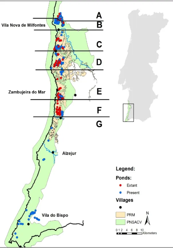
Figure 1: Study area. In blue are the ponds that still persists in 2009, in red the ponds destroyed. The implantation of the irrigation beneficiation perimeter (PRM) is showed in orange and the natural park in Green. Main villages in the study area are also represented.

holbrooki) are common in the irrigation channels and frequently colonize the more permanent ponds and streams.

2.2. Sampling design 2.2.1. Pond survey

We conducted a pond survey during the winter of 2008/2009, using aerial photography and 1:25,000 topographic maps, and crosschecked with similar surveys made 1991, 1993, 1996 and 2000 (Faria et al. 1993; Silva 1998; Gordo & Galera 2000). We visited every site that was identified in the previous surveys and recorded it state: present or destroyed, and the apparent reason for it (drained, plowed, cultivated, constructed, etc.), or converted to reservoir. We defined temporary ponds as bodies of water occupying depressions, which are flooded during the rainy season for a sufficiently long period to allow the development of aquatic vegetation and hydromorphic soils, but which are not in contact with permanently flooded habitats such as rivers.

2.2.2. Amphibian sampling

We sampled five habitats to understand how this amphibian community uses the availed habitats: temporary ponds, streams, agricultural reservoirs, irrigation channels and ditches. The temporary ponds sampled were the ponds selected and sampled by Beja & Alcazar (2003) that still subsisted in 2010. We selected the remaining sites using the same seven north-south divisions (sectors A’ to G’) of the coastal plateau used in the same study. For each sector, four sites of each type of habitat were randomly selected from at least eight possible alternative sites that we recognized in the spring of 2009, and that were at least 500 m a part of each other. We only sampled streams that run directly to the sea. The irrigation channels were made of concrete. In some divisions there were not four sites of each habitat to be sampled. The streams were not evenly distributed across the study area, and we only sampled ditches and irrigation channels inside of the PRM. A total of 122 sites were sampled: 38 temporary ponds, 31 reservoirs, 21 streams, 17 ditches and 15 irrigation channels.

We sampled for amphibians in four discrete periods during the wet season of 2010: 1) 6 to 16 of February and 4 to 6 of March; 2) 13 to 26 of March; 3) 24 of April to 5 of May; 4) 8 to 13 of July. These periods match the main reproductive activity of the amphibian present in that area (Ferrand et al. 2001). Depending on the water available in the site, each sample consisted of three to six 30’s blind sweeps (mean=3.1, SD=0.6, n=362) with a 30*20 cm aperture dip-net, conducted by one person wading across the site and systematically covering all habitats available. Amphibian larvae were identified to species and returned to water at the end of each sampling session; tree frog tadpoles (Hyla spp.) could not be reliably separated in the field and were thus identified to genus. Adults of Caudata found during sweeps were assumed that were reproducing and were include as present.

2.3. Data analysis 2.3.1. Pond persistence

We analyzed the pond persistence using a Cox proportional hazards regression model (PHR; (Cox 1972), using the statistical software package “Survival” (Therneau & Lumley 2012), an add-on to R software (R Development Core Team 2011), to determine if there were significant differences on the surviving function of the ponds inside and outside of the PRM and of the PNSACV. Because data for the ponds persistence was not available for every year, we assumed that ponds that were destroyed between two surveys have survived half of the period between the two surveys. For example, a pond that was present in 1996 and destroyed in 2000, we assumed that it was destroyed in 1998. We built four models, the Null, one for each variable (PRM and PNSACV, dummies variables with 1 = inside and 0 = outside of PRM and PNSACV respectively), and a “full model” using both variables (PRM + PNSACV). We compared the models using aikaike’s information criteria (Burnham & Anderson 2002).

2.3.2. Multispecies-multiseason model of occupancy

Occupation of different habitats by the amphibian community of the southwest of Portugal was assessed using an extension of the single-species, dynamic occupancy model developed by MacKenzie et al. (2003) as proposed by (Dorazio et al. 2010): a hierarchical (or state–space) formulation that includes distinct models of species occurrence and species detection given occurrence. This approach allows the specifying of models for species occurrences and their potential ecological determinants (habitat or other site-level covariates) independent of the effects of imperfect detection. The imperfect detection is specified in a second component of the model, the observation process, wherein detections of species are modeled conditional on latent species occurrence (or occupancy state) parameters.

Let T denote the number of distinct (i.e., non-overlapping) k periods in which the metacommunity is sampled. Let S be the number i sites (corresponding to S local communities) that were surveyed. Let Zi,1,l denote the true occupancy state of species l (in a total of N species in the community) in site i during the first period, wherein indicates presence and indicates absence. We modeled this initial occupancy (occupancy during period 1) as an outcome of a Bernoulli trial:

( ) (Eq. 1)

Where ( | ) denotes the probability that species l is present (i.e. occupancy probability) at location i during period 1 given the location has water during period k. Here { } denotes a latent variable that indicates if the ith location has water to support amphibian reproduction and/or larvae dwelling in the k period. Note if (i.e. the location i has no water during period k), then with probability one.

We assumed that occupancy in the following periods will depend on the occupancy state in the previous period, as follows:

( ( ( ))) (Eq. 2)

(for k = 1, …, T – 1) where ( ) denotes the conditional probability of the species l will arrive and occupy location i in period k + 1 given that it was absent in the previous sampling period and that the location has water in period k +1. Dorazio et al. (2010) refer to this event as local colonization, although we kept this notation we don’t expect that this event will always correspond to the arrival of a species to a new location where it had become extinct before. As we sampled in one year during the breeding season this event will more likely represent the arrival of a late breeder to the breeding site.

The parameter ( ) denotes the conditional probability of species l still persist in site i during period k + 1 given that it was present in the previous period and that the location i has water in period k + 1. We refer to this event as persistence. The complementary event is denominated local extinction, it can be expressed as follows: . Although this event could correspond to a proper event of extinction, again, it is more likely to correspond to the event of a species leaving the breeding site because all individuals had finished their metamorphosis and began to disperse to the surroundings. The occupancy probability of species l in the ith site in period 2 to T is expressed as follows: ( ) (for k = 1, …, T – 1).

We assumed that these probabilities ( ) are function of the habitat. We incorporate these effects in the model using the logit link function (Kéry & Royle 2008; Russell et al. 2009; Zipkin et al. 2010). Let vim be a site-covariate that identifies if site i belongs to the type of habitat m. The initial occupancy probability was calculated as follows:

( ) ∑

(Eq. 3)

(for m =1,…, Hb, where Hb is the total number of habitat types, 5 in our study). b0l denotes the baseline, at logit-scale, probability for occupancy in the first period for species l, blm the effect of habitat m in initial occupancy probability of species l. Likewise, and keeping the same notation, the colonization and persistence probability were calculated as:

( ) ∑

(Eq. 4)

( ) ∑

(Eq. 5)

(for k =1, …, T -1). Note that the baseline (c0 and d0) are specie and period specific, but we assumed that the habitat effect is constant for each species across all periods.

True occurrence is imperfectly observed, which confounds the estimation of and the others parameters. However, sampling at a point i with J > 1 replicates over a short period (such that the community remains closed for the duration of the survey) allows for a formal distinction between species absence and non-detection (MacKenzie et al. 2002). We assumed that the J replicates are independent, that the detectability does not change and that the stock of the larvae doesn’t exhaust until all J replicates are done. J was not constant across sites and periods and that do not interfere with model (Dorazio et al. 2010). For each i site, k period and l specie we observe an encounter history ( ), that consist of J binary observations that indicate whether specie l was detected ( ) or not detected ( ) during the jth observation in site i, during period k. For example, Y = (0, 1, 1, 0, 1) indicates a specie that was detected in three sweeps, the second, the third and fifth, in a total of five sweeps.

The detection of species is dependent on whether a species is present or not. The occupancy state is only partially observed due to the ambiguity of an all-zero encounter history, i.e. y = 0 can happen if a species is really absent or if it

is present but remained undetected. We modeled the encounter history as an outcome of a Bernoulli trial:

( ) (Eq. 6)

Where ( ) denotes the conditional probability of detecting the lth _{species during the j}th _{observation in site i during period k given} that the species is present. Thus if the specie l is absent of site i in period k then for every j sweep with probability one; otherwise the specie will be detected with probability.

Similarly with the other probabilities, we assumed that the probability of detection, , is function of the habitat and we modeled likewise with the equations 3-5:

( ) ∑ (Eq. 7)

(for k= 1 , …, T), where a0lk denotes the baseline, at the logit scale, for the detection of of specie l at period k, and alm the effect of habitat m in the detection probability of species l. Similarly with colonization and persistence parameters, the baseline it is specie and period specific and the effect of the habitat is constant for each species across all periods.

Because this model has many parameters and some species are detected infrequently, or not all in some habitats, estimating of all the model parameters was impossible unless we made further assumptions. We assumed that the community of amphibians of the southwest of Portugal responds in similar way, not equal, in the choice of breeding habitat. We illustrate this approach using the parameters in equation 3, b0l and blm. We assumed that these parameters are drawn from higher level parameters:

( )(Eq. 8)

( )(Eq. 9)

mean of this distribution, ⁄ , can be viewed as “mean” initial occupancy for every species. Similarly to this, is the parameter of the exponential distribution of witch the effects in the initial occupancy of the habitat m in species l is taken. Again the mean, ⁄ , can be viewed as “mean” effect of habitat m in the initial occupancy for all the species. This “hyper-parameters” increase the precision of the estimation of the parameters of the rarer species. We modelled inter-specific variation in the parameters associated with probabilities of colonization, persistence and detectability in the same way. We assumed that distribution of the parameters is asymmetric (exponential) instead of a symmetric distribution (normal) as used in others studies (e. g. Zipkin et al. 2010; Dorazio et al. 2010). Assuming a normal distribution of the priors would estimate the parameters of the rarer species to be closer to the mean of the community, thus overestimating their occupancy and the species richness of the sites where more species occur.

Because true occupancy was calculated by location, period and species (Zikl), the estimation of relevant community parameters is easily estimated. For the analyses of the occupancy the amphibian community in Southwest Portugal we estimated the species richness per site (Rqi), mean richness per habitat across all periods (m.Rqm) and mean habitat richness per habitat and per period (mk.Rqm,k): ∑ ( ) (Eq. 10) (For i=1, …, S) ∑ ( ) ∑ (Eq. 11) ∑ _∑ ∑ (Eq. 12) (For k=1, …, T and m=1, …, Hb)

The habitats mean occupation (Occmkl) and detection probability (p.meanmkl) per period and species:

∑

∑ (Eq. 13)

∑

∑ (Eq. 14)

(For k=1, …, T; l=1, …, N and m=1, …, Hb)

Because our multispecies, multiseasons model have many latent parameters we opted by Bayesian approach using Markov Chain Monte Carlo (MCMC). Our inferences are based only in a large sample of the joint posterior distributions of the model’s parameters.

We fit our model using the free software WinBUGS (Lunn et al. 2009). Because using BUGS natively can be challenging (Kéry 2010), we implanted the model in R (R Development Core Team 2011), call WinBUGS through the package R2WinBUGS (Sturtz et al. 2005), and handled the results back in R. We run three chains of a length of 200,000 iterations after a burn in of 100,000, we then thinned the chains by 10. Convergence was assessed using the R-hat statistic, which examines the variance ratio of the MCMC algorithm within and between chains across iterations (see Appendix 1 in Supplementary material for WinBUGS code).

3. Results

3.1. Pond persistence

From the 296 sites identified in the five surveys that had temporary ponds in 1991, only 165 were present in 2009, representing a pond loss of over 44%. A total of 25 ponds were identified out of PNSACV, of which only three were lost between 1991 and 2009. Inside the PNSACV the loss of ponds was 47%. The main loss of ponds was observed inside the PRM, where 59% were lost, against 21% of loss outside the PRM (Table 1). The main loss was observed in the period between 2000 and 2009, corresponding to a 30% loss.

The main cause for pond destruction was the use for agricultural purposes, corresponding to 90 ponds (68.7%). Usually the terrain was drained and the site

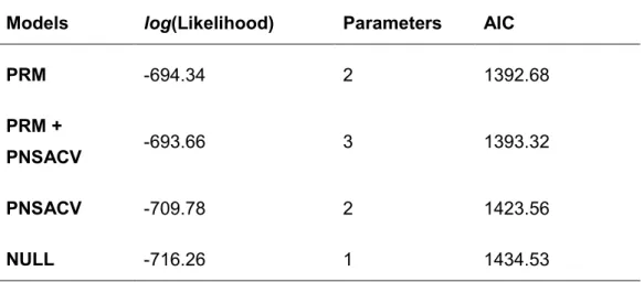
reservoirs was the second most common cause of destruction, corresponding to 22 ponds. A total of seven sites were encroached by Acacia sp. There were was also five ponds drained, five sites that now have constructions, one under a forest plantation, and one that was converted into a dumping site (Figure 2). The PHR models constructed were all better than the null model, with the Likelihood-ratio test always rejecting the null model in favor of the alternative model. The models that scored least in the Aikaike information criteria (AIC, Burnham & Anderson 2002) were those including the variable PRM (Table 2). In the “full model” the variable PNSACV was not statistically significant (p = 0.281). The ponds inside the PRM have lower survival probability (in 2009, p= 0.414) than the ponds outside of the PRM (in 2009, p= 0.775; Figure 3).

3.1. Habitat occupancy

During the sampling season, 1357 sweeps were made, in which there were detected amphibians in 562, capturing 20864 individuals in 83 locations. The most common taxa found was the western spadefoot toad (Pelobates cultripes),

Table 1: Number of temporary lagoons present in study area between 1991 and 2009. In and out of Parque Natural do Sudoeste Alentejano e Costa Vicentina (PNSACV); and In and out of Perímetro de Rega do Mira (PRM). The PRM is mainly within the PNSACV.

1991 1993 1996 2000 2009 PNSACV Out 25 24 23 23 22 In 271 249 221 214 143 PRM Out 84 83 78 77 66 In 187 166 143 137 77 Total 296 273 244 237 165

frog (Discoglossus galganoi), for which we found only seven individuals in two locations. The most ubiquitous species was the green frog (Pelophylax perezi), which found in every habitat except the temporary ponds. The habitats where more species were observed were the temporary ponds and the reservoirs, with seven species each. However, the proportion of temporary ponds occupied by amphibians (0.95) was much higher than that of reservoirs (0.61). The irrigation channels were the habitat with less species observed (Table 3).

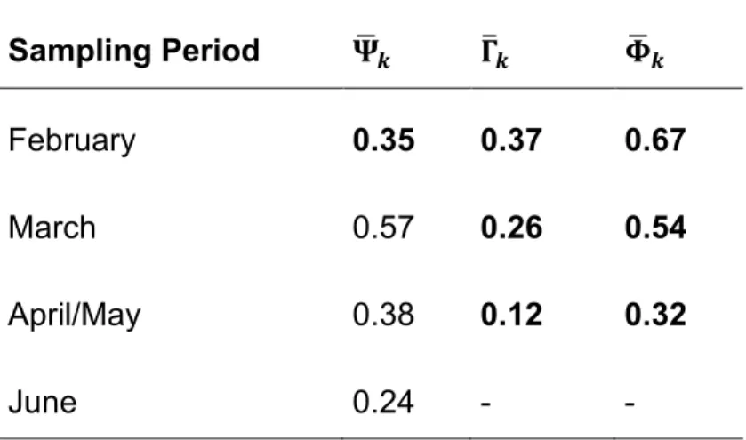
We used the hyper parameters of the model as a surrogate for the community parameters. The mean occupancy probability peaked in March ( ̅). The mean colonization probability ( ̅) and the mean persistence probability ( ̅) declined across the sampling season (Table 4). The mean detection probability was 0.32. The mean effects of the habitats in the initial occupancy ( ̅), the colonization probability ( ̅), the persistence probability ( ̅) and the detection probability ( ̅) are listed in Table 5.

The mean richness of each habitat calculated by dynamic occupation model was always greater than the mean richness observed (Figure 4). The temporary ponds were the habitat that was able to sustain more species per site. The

Farmed Dredged Shrub Encroachment Construction Drained Dumping Forested

Figure 2: Causes for the destruction of the 131 temporary ponds found destructed in southwest of Portugal by 2009.

irrigation channels and ditches were the poorest habitats, and usually they did not support more than one or two species. Reservoirs were occupied by some of the more plastic species. Although streams have a low observed mean richness, the model calculated the second highest mean richness.

The detection probability of the species was difficult to calculate in the habitats where the species were never detected. The values calculated for these parameters were near zero and showed large credible intervals. In general, the detection of the specie was similar across the habitats where the species was detected, though ponds tended to be the habitat were species were detected more easily (larger detection probability, see Appendix 2 in Supplementary material).

The species occurrence varied between habitats and across the breeding season. In general, species had larger occupancy rates in ponds, with the highest values in March or April and subsequent declines thereafter. The spadefoot toad, the tree frog, the ribbed salamander (Pleurodeles waltl), the Bosca’s newt (Lissotriton boiscai) and the small marbled newt (Triturus pygmaeus) occupied some reservoirs. Although the occupancy of the reservoirs was always low, it did not decline in June (Figure 4a). The natterjack toad (Epidalea calamita) and the parsley frog (Pelodytes punctatus) seem not to be

Table 2: The log likelihood, number of parameters and the akaike information criterion score (AIC) of the Cox partial hazards regression models (PHR) constructed to analyze the survival of ponds in Southwest of Portugal.

Models log(Likelihood) Parameters AIC

PRM -694.34 2 1392.68

PRM +

PNSACV -693.66 3 1393.32

PNSACV -709.78 2 1423.56

able to occupy the reservoirs, but, at least the natter jack toad, can occupy the ditches. These species are absent from the later periods (Figure 4b). There are also the later breeders, like the green frog, that occupy preferably the more persistent habitats like the reservoirs and the irrigation channels. Occupancy by these species did not decline at the end of breeding season (Figure 4c). Three species consistently occupied streams: the common toad (Bufo spinosus), the green frog and the Bosca’s newt (see appendix in the Supplementary material).

Figure 3: Survival function of the ponds of southwest Portugal, between 1991 and 2009, inside and outside the Mira Irrigation Perimeter (PRM). The gray lines represent de 95% confidence interval.

Temporary ponds were always the habitat with higher species richness across all study period. The others habitats seldom have more than one species per site (Figure 4d).

4. Discussion

4.1. Pond loss due to agriculture pressure

There are about 277,400,000 ponds in the world with area equal to one hectare or less, covering, about 692,600 km2 (Downing et al. 2006). This and the fact that ponds contribute to regional diversity more than other water bodies (Williams 2004; Davies et al. 2008), make ponds an important habitat even that

Table 3: Number of sites where species were observed. Between brackets observed occupancy.

Species Ponds _(n=38) Reservoir _(n=31) Streams _(n=21) Ditches _(n=17) Channels _(n=15)

Caudata Lissotriton boscai 11 (0.29) 1 (0.03) 4 (0.19) 0 (0.00) 0 (0.00) Peleurodeles waltl 32 (0.84) 7 (0.23) 0 (0.00) 0 (0.00) 0 (0.00) Triturus pygameus 20 (0.53) 7 (0.23) 0 (0.00) 0 (0.00) 0 (0.00) Anura Bufo spinosus 0 (0.00) 8 (0.26) 7 (0.33) 0 (0.00) 1 (0.07) Epidaleia calamita 18 (0.47) 0 (0.00) 0 (0.00) 6 (0.35) 0 (0.00) Discoglossus galganoi 0 (0.00) 0 (0.00) 1 (0.05) 1 (0.06) 0 (0.00) Hyla spp. 32 (0.84) 7 (0.23) 0 (0.00) 1 (0.06) 0 (0.00) Pelobates cultripes 35 (0.92) 8 (0.26) 0 (0.00) 1 (0.06) 0 (0.00) Pelodytes puntactus 30 (0.79) 0 (0.00) 0 (0.00) 1 (0.06) 0 (0.00) Pelophylax perezi 0 (0.00) 12 (0.39) 6 (0.29) 4 (0.24) 6 (0.40) Sites with Amphibians 36 (0.95) 19 (0.61) 12 (0.57) 9 (0.53) 7 (0.47)

Miracle et al. 2010). Ponds, natural and manmade, are disappearing from several parts of the world (Hull 1997; Beebee 1997; King 1998; Boothby 2003; Curado et al. 2011) and Portugal is no exception. What is of major concern is the fact is this loss happens inside of a protected area, though this happens, mostly, because the Mira beneficiation perimeter is almost all within the natural park.

The intensification of agriculture that have been witness in this region (Beja & Alcazar 2003; Pita et al. 2006) was responsible for the destruction of the great majority of the ponds present in Southwest of Portugal (89% = agriculture + dredging + draining). Agriculture is the major threat to ponds in the Mediterranean region (Dimitriou et al. 2006). The lower survival probability of the ponds inside of irrigation perimeter reflects a land use management that is more focused in agricultural production than on biodiversity conservation.

4.2. Dynamic occupation of aquatic habitats

The highest species richness in Southwest of Portugal was found in temporary

Table 4: Community parameters: ̅ was the mean occupation probability for the amphibian community in period k. ̅and ̅ are the mean colonization and the mean persistence probability between period k and k+1. The values in bold are median estimates taken from the dynamic occupation model. The subsequent mean occupancy were calculated as follows:

̅ ₍ ̅ ) ̅ ̅ ̅ . Sampling Period ̅ ̅ ̅ February 0.35 0.37 0.67 March 0.57 0.26 0.54 April/May 0.38 0.12 0.32 June 0.24 - -

habitat for amphibians in the Mediterranean region (Diaz-Paniagua 1990). The alternation between a wet state and dry state promotes the development of high diversity communities, due to lack of competitors and/or predators (Beja & Alcazar 2003; Pinto-Cruz et al. 2009). Amphibians are able to minimized the competition between species by choosing different timings for reproduction (Jakob et al. 2003; Richter-boix et al. 2006b).

Few species were found to occupy the streams, though it is possible that we failed to detect some species. The streams in Southwest Portugal have a high incidence of fishes and of the exotic predator Procambarus clarkii. This was already associated with depletion of species in amphibian communities in Californian streams (Riley et al. 2005). The presence of fishes and crayfishes was also high in channels and ditches, present in almost every site observed (pers. obs.). The presence of these predators seems to be enough to keep most species from occupying these habitats. The natter jack toad and the green

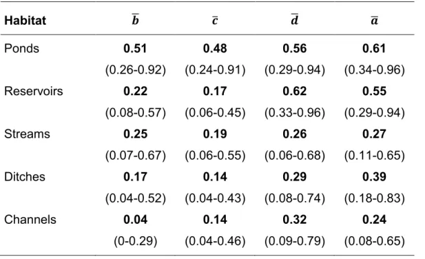
Table 5: Median of dynamic occupation model (hyper) parameters for mean effects of the habitats in the initial occupancy ̅, the colonization probability ̅, the persistence probability ̅ and the detection probability ̅. Between brackets the 95% credible interval (CI).

Habitat ̅ ̅ ̅ ̅ Ponds 0.51 (0.26-0.92) 0.48 (0.24-0.91) 0.56 (0.29-0.94) 0.61 (0.34-0.96) Reservoirs 0.22 (0.08-0.57) 0.17 (0.06-0.45) 0.62 (0.33-0.96) 0.55 (0.29-0.94) Streams 0.25 (0.07-0.67) 0.19 (0.06-0.55) 0.26 (0.06-0.68) 0.27 (0.11-0.65) Ditches 0.17 (0.04-0.52) 0.14 (0.04-0.43) 0.29 (0.08-0.74) 0.39 (0.18-0.83) Channels 0.04 (0-0.29) 0.14 (0.04-0.46) 0.32 (0.09-0.79) 0.24 (0.08-0.65)

natter jack toad is an opportunist reproducer with small metamorphic size that can use more ephemeral water bodies (reviewed in Jakob et al. 2003) and probably occupies the more temporary ditches to reduce intraspecific competition. Ditches are made for draining water, often with fertilizers and pesticides, from agricultural field and should be of lower water quality.

The green frog is associated with permanent water bodies (Diaz-Paniagua 1990) and in this study was the species that was found in all habitats except temporary ponds. It was also the species that reproduce in more sites, even

Figure 4: Mean amphibian richness per habitat. The first, the median and the third quartile define the box. The whiskers represent the 95% credible intervals (CI). The circles are the mean of the observed amphibian richness per habitat.

these predators could explain why the green frog was the only species to occupy the channels. It is a very tolerant species to pesticides, like the copper sulfate, and is the most common species in altered wetlands (García-Muñoz et al. 2009). The absence from temporary ponds could be explained as part of strategy to avoid interspecific competition or as late breeder (Diaz-Paniagua 1992), the temporary ponds may not have the necessary water to support green frog larvae development.

Figure 5: Mean occurrence of a) Pelobates cultripes; b) Epidalea calamita and c) Pelophylax

perezi and the d) mean richness per habitat and across the study period. The circles represent

the ponds; the squares, the reservoirs; the diamonds, the streams; triangles represent ditches and inverted triangles, the irrigation channels. The full shapes represent the median of the model estimates and the void shapes the observed values. The gray bars represent the 95% credible intervals (CI).

Agricultural reservoirs are increasing worldwide (Downing et al. 2006) and are usually regarded as important alternative habitat for amphibians, at least in agricultural regions where wetlands are scarce (Knutson et al. 2004). In the Southwest of Portugal, only a sub-set of four pond-dwelling species are able to occupy a small number of the reservoirs studied (Hyla spp., Pelobates cultripes, Pleurodeles waltl and Triturus pygmaeus). In addition to this sub-set, two more species occupied the reservoirs: the common toad and green frog. It is surprising that the mean richness per site was low (maximum of 1.4 (CI at 95% = 1.1 - 2.3) in March). In previous studies the presence of exotic predators, did not fully explained the lower abundance and surviving rate of amphibians in permanent versus temporary ponds (Adams 2000). Probably some feature (e.g.: water temperature and or quality, food shortage, plant community) related to the permanent character of the reservoirs does not allow species of amphibians to occupy these habitats as efficiently as temporary ponds. Knutson et al. (2004) argues that the best reservoirs for sustaining amphibians should be small, with no fish and with small concentrations of nitrogen.

Species detection probability changed between habitats and across seasons. Not explicitly accounting for this source of biases would make impossible for formally compare such different habitats. The dynamic formulation of the occupation state of the sites allowed for the breeding phenology of this amphibian community to be modeled, accounting for earlier and later breeders in the site richness. Some species had too little detection in some habitats that would be impossible to estimate the occurrence using single-species models. Assuming that the species parameters were taken from an asymmetric distribution allowed that some parameters could take the values of zero, or near, and not being over-estimated when pulled by the mean.

4.3. Implication for conservation

This study shows that this community preferably occupies the temporary ponds for reproduction. The association described between the Mediterranean amphibian community and temporary ponds (Diaz-Paniagua 1990; Beja &

suggests that these species are adapted to reproduce in temporary ponds. It is not expectable that as new water habitats appear that amphibians would occupy them if they do not meet the conditions for their reproduction. With the loss of temporary ponds due to agricultural pressure, there is no alternative habitat to support the diversity of this amphibian community.

The loss of the ponds is not random across the study area (Figure 1). Ponds occur generally in clusters and agricultural fields are managed by the parcel. When a parcel is chosen to be intensified, all ponds present in the parcel are destroyed. Parcels selected to be intensified are usually inside the irrigation perimeter. If the rate of destruction of ponds inside the irrigation perimeter does not halt soon, several species will disappear from the coastal plateau, or at least will see their breeding habitat severely reduced. With the loss of the ponds inside of the PRM, the two populations outside, north of the river Mira and Vila do Bispo, will become more isolated and therefore more susceptible stochastic extinctions and inbreeding depression.

The conservation of this community of amphibians passes by conserving the remaining temporary ponds of this region and by recovering the ponds that were lost inside the irrigation perimeter. The amphibians respond well to restoration of wetlands as long as some aspects are taken to account: maintain a temporal characteristic, avoid the introduction of fish and other predators, maintain a terrestrial habitat that allows the wintering and dispersal of adults and a small distance to source population (reviewed in Brown et al. 2012). The construction of ponds should be in clusters, and every cluster should have ponds with different depths and margins configurations, as the requirement of each species is not fully know this will create a gradient of hydroperiod and a diversity of aquatic mesohabitat to satisfy every species (Rannap et al. 2009). Cattle should not access the ponds during the flooded season, to avoid an increase of nitrogen in the ponds and to prevent diseases in cattle (Knutson et al. 2004). The conservation efforts should be concentrated in the remaining clusters of ponds inside the irrigation perimeter and in recovering of clusters of ponds nearby.

Acknowledgments:

This study was financed in part by an FCT project “Spatial structure of amphibian (meta)populations in Mediterranean farmland: implications for conservation management” (PTDC/BIABDE/68730/2006 - Ciências Biológicas - Biodiversidade e Ecologia).

The author would like to thank to Sara and my family for the support; to Paulo Cabrita, Filipa Oliveira, Cândida Delgado, Sara Ivone and Francisco Silva for the help with sampling; to Carlos Vila-Viçosa, Mirjam van de Vliet, Carla Pinto-Cruz and Paula Canha for the insights; to Marc Kéry for the support and suggestions for the WinBUGS code; to Miguel Porto for the support with the R program; to Hugo Rebelo and Luis Reino in CIBIO-Lisboa for the exchange of ideas; to Pedro Beja for accepting me for advising and to Joana Santana and Paulo Sá-Sousa for reviewing this thesis.

References:

Adams, M. 2000. Pond permanence and the effects of exotic vertebrates on anurans. Ecological Applications 10:559-568.

Alford, R. A., and S. J. Richards. 1999. Global amphibian declines: a problem in applied ecology. Annual Review of Ecology and Systematics 30:133–165. JSTOR.

Barrett, K., and C. Guyer. 2008. Differential responses of amphibians and reptiles in riparian and stream habitats to land use disturbances in western Georgia, USA. Biological Conservation 141:2290-2300.

Beebee, T. J. C. 1997. Changes in dewpond numbers and amphibian diversity over 20 years on chalk downland in Sussex, England. Biological

Conservation 81:215-219.

Beja, P., and R. Alcazar. 2003. Conservation of Mediterranean temporary ponds under agricultural intensification: an evaluation using amphibians. Biological Conservation 114:317-326.

Billeter, R. et al. 2008. Indicators for biodiversity in agricultural landscapes: a pan-European study. Journal of Applied Ecology 45:141-150.

Blaustein, A. R., B. a Han, R. a Relyea, P. T. J. Johnson, J. C. Buck, S. S. Gervasi, and L. B. Kats. 2011. The complexity of amphibian population

declines: understanding the role of cofactors in driving amphibian losses. Annals of the New York Academy of Sciences 1223:108-19.

Boothby, J. 2003. Tackling degradation of a seminatural landscape: options and evaluations. Land Degradation & Development 14:227-243.

Brand, A. B., and J. W. Snodgrass. 2010. Value of artificial habitats for amphibian reproduction in altered landscapes. Conservation Biology

24:295-301.

Brown, D. J., G. M. Street, R. W. Nairn, and M. R. J. Forstner. 2012. A Place to Call Home: Amphibian Use of Created and Restored Wetlands.

International Journal of Ecology 2012:1-11.

Burnham, K., and D. R. Anderson. 2002. Model selection and multimodel inference: a practical information-theoretic approach2nd ed. Springer-Verlag.

Collins, J. P. J. P., and A. Storfer. 2003. Global amphibian declines: sorting the hypotheses. Diversity and Distributions 9:89–98.

Cox, D. R. 1972. Regression Models and Life-Tables. Journal of the Royal Statistical Society. Series B (Methodological) 34:187-220.

Crawford, J. A., and R. D. Semlitsch. 2007. Estimation of core terrestrial habitat for stream-breeding salamanders and delineation of riparian buffers for protection of biodiversity. Conservation Biology 21:152-8.

Cruz, M. J., R. Rebelo, E. G. Crespo, and E. G. Crespo. 2006. Effects of an introduced crayfish, Procambarus clarkii , on the distribution of south-western Iberian amphibians in their breeding habitats. Ecography 29:329-338.

Curado, N., T. Hartel, and J. W. Arntzen. 2011. Amphibian pond loss as a function of landscape change – A case study over three decades in an agricultural area of northern France. Biological Conservation 144:1610-1618.

Céréghino, R., J. Biggs, B. Oertli, and S. Declerck. 2007. The ecology of European ponds: defining the characteristics of a neglected freshwater habitat. Hydrobiologia 597:1-6.

Davies, B., J. Biggs, P. Williams, M. Whitfield, P. Nicolet, D. Sear, S. Bray, and S. Maund. 2008. Comparative biodiversity of aquatic habitats in the

European agricultural landscape. Agriculture, Ecosystems & Environment

Diaz-Paniagua, C. 1990. Temporary ponds as breeding sites of amphibians at a locality in southwestern Spain. Herpetological Journal 1:447–453. British Herpetological Society.

Diaz-Paniagua, C. 1992. Variability in timing of larval season in an amphibian community in SW Spain. Ecography 15:267-272.

Dimitriou, E., I. Karaouzas, N. Skoulikidis, and I. Zacharias. 2006. Assessing the environmental status of Mediterranean temporary ponds in Greece. Annales de Limnologie - International Journal of Limnology 42:33-41. Dorazio, R. M., M. Kéry, J. A. Royle, and M. Plattner. 2010. Models for

inference in dynamic metacommunity systems. Ecology 91:2466-75.

Downing, J. a., Y. T. Prairie, J. J. Cole, C. M. Duarte, L. J. Tranvik, R. G. Striegl, W. H. McDowell, P. Kortelainen, N. F. Caraco, and J. M. Melack. 2006. The global abundance and size distribution of lakes, ponds, and impoundments. Limnology and Oceanography 51:2388-2397.

Faria, F., P. Cabrita, and M. J. Gonçalves Pinto. 1993. Cartografia de Lagoas Temporárias da APPSACV. Odemira.

Ferrand, N., P. Ferrand, H. Gonçalves, F. Sequeira, J. Teixeira, and F. Ferrand de Almeida. 2001. Guia FAPAS Anfibios e Répteis de Portugal.

FAPAS/Camara Municipal do Porto, Porto.

Ficetola, G. F., F. De Bernardi, and F. D. Bernardi. 2004. Amphibians in a human-dominated landscape: the community structure is related to habitat features and isolation. Biological Conservation 119:219-230.

Ficetola, G. F., E. Padoa-Schioppa, F. De Bernardi, V. Celoria, and P. Scienza. 2008. Influence of landscape elements in riparian buffers on the

conservation of semiaquatic amphibians. Conservation Biology 23:114-23. García-Muñoz, E., J. D. Gilbert, G. Parra, and F. Guerrero. 2009. Wetlands

classification for amphibian conservation in Mediterranean landscapes. Biodiversity and Conservation 19:901-911.

Gordo, A. R., and M. L. O. Galera. 2000. Caracterização Ecológica das Lagoas Temporárias da Costa Sudoeste. Odemira.

Gómez-Rodríguez, C., C. Díaz-Paniagua, L. Serrano, M. Florencio, A. Portheault, and Æ. C. Dı. 2009. Mediterranean temporary ponds as

amphibian breeding habitats: the importance of preserving pond networks. Aquatic Ecology 43:1179-1191.

Hamer, A. J., and M. J. Mcdonnell. 2008. Amphibian ecology and conservation in the urbanising world: A review. Biological Conservation 141:2432-2449.

Hartel, T., O. Schweiger, K. Öllerer, D. Cogălniceanu, and J. W. Arntzen. 2010. Amphibian distribution in a traditionally managed rural landscape of

Eastern Europe: Probing the effect of landscape composition. Biological Conservation 143:1118-1124.

Hayes, T. B., P. Falso, S. Gallipeau, and M. Stice. 2010. The cause of global amphibian declines: a developmental endocrinologist’s perspective. The Journal of Experimental Biology 213:921-33.

Hull, A. 1997. The pond life project: a model for conservation and sustainability. Pages 101–109 in J. Boothby, editor. British Pond Landscapes. Action for Protection and Enhancement. Proceedings of the UK Conference of the Pond Life Project. Pond Life Project, Liverpool.

Jakob, C., G. Poizat, M. Veith, A. Seitz, and A. J. Crivelli. 2003. Breeding phenology and larval distribution of amphibians in a Mediterranean pond network with unpredictable hydrology. Hydrobiologia 499:51-61.

King, J. 1998. Loss of diversity as a consequence of habitat destruction in California vernal pools. California Native Plant Society, Sacramento, California:119-123.

Knutson, M. G., W. B. Richardson, D. M. Reineke, B. R. Gray, J. R. Parmelee, and S. E. Weick. 2004. Agricultural Ponds Support Amphibian Populations. Ecological Applications 14:669-684.

Kéry, M. 2010. Introduction to WinBUGS for Ecologists: Bayesian Approach to Regression, ANOVA, Mixed Models and Related Analyses, 1st edition. Elsevier, Amsterdam.

Kéry, M., and J. A. Royle. 2008. Hierarchical Bayes estimation of species richness and occupancy in spatially replicated surveys. Journal of Applied Ecology 45:589-598.

Lunn, D., D. Spiegelhalter, A. Thomas, and N. Best. 2009. The BUGS project: Evolution, critique and future directions. Statistics in Medicine 28:3049-67. MacKenzie, D. I., J. D. Nichols, J. E. Hines, M. G. Knutson, and A. B. Franklin. 2003. Estimating Site Occupancy, Colonization, and Local Extinction When a Species is Detected Imperfectly. Ecology 84:2200-2207.

MacKenzie, D. I., J. D. Nichols, G. B. Lachman, S. Droege, J. Andrew Royle, and C. A. Langtimm. 2002. Estimating site occupancy rates when detection probabilities are less than one. Ecology 83:2248-2255.

Maes, J., C. J. M. J. M. Musters, G. R. De Snoo, and G. R. D. Snoo. 2008. The effect of agri-environment schemes on amphibian diversity and abundance. Biological Conservation 141:635-645.

Mazerolle, M. J. M. J., L. L. Bailey, W. L. Kendall, J. Andrew Royle, S. J. S. J. Converse, and J. D. J. D. Nichols. 2007. Making great leaps forward: accounting for detectability in herpetological field studies. Journal of Herpetology 41:672–689.

Miracle, M. R., B. Oertli, R. Céréghino, and A. Hull. 2010. Preface: conservation of european ponds-current knowledge and future needs. Limnetica 1:1–9. Neto, C., J. Capelo, C. Sérgio, and J. C. Costa. 2007. The Adiantetea class on the cliffs of SW Portugal and of the Azores. Phytocoenologia 37:221-237. Oertli, B., J. Biggs, R. Céréghino, P. Grillas, P. Joly, and J.-B. Lachavanne.

2005. Conservation and monitoring of pond biodiversity: introduction. Aquatic Conservation: Marine and Freshwater Ecosystems 15:535-540. Oertli, B., R. Céréghino, A. Hull, and R. Miracle. 2009. Pond conservation: from

science to practice. Hydrobiologia 634:1-9.

Pinto-Cruz, C., J. a. Molina, M. Barbour, V. Silva, and M. D. Espírito-Santo. 2009. Plant communities as a tool in temporary ponds conservation in SW Portugal. Hydrobiologia 634:11-24.

Pita, R., P. Beja, and A. Mira. 2007. Spatial population structure of the Cabrera vole in Mediterranean farmland: The relative role of patch and matrix effects. Biological Conservation 134:383-392.

Pita, R., A. Mira, and P. Beja. 2006. Conserving the Cabrera vole, Microtus cabrerae, in intensively used Mediterranean landscapes. Agriculture, Ecosystems & Environment 115:1-5.

R Development Core Team. 2011. R: A Language and Environment for Statistical Computing. R Foundation for Statistical Computing, Vienna - Austria.

Rannap, R., A. Lõhmus, and L. Briggs. 2009. Restoring ponds for amphibians: a success story. Hydrobiologia 634:87-95.

Ribeiro, R., M. a. Carretero, N. Sillero, G. Alarcos, M. Ortiz-Santaliestra, M. Lizana, and G. a. Llorente. 2011. The pond network: can structural connectivity reflect on (amphibian) biodiversity patterns? Landscape Ecology 26:673-682.

Richter-boix, A., G. A. Llorente, and A. Montori. 2006a. Breeding phenology of an amphibian community in a Mediterranean area. Amphibia-Reptilia

27:549-559.

Richter-boix, A., G. A. Llorente, and A. Montori. 2006b. A comparative analysis of the adaptive developmental plasticity hypothesis in six Mediterranean

anuran species along a pond permanency gradient. Evolutionary Ecology Research 8:1139-1154.

Riley, S. P. D., G. T. Busteed, L. B. Kats, T. L. Vandergon, L. F. S. Lee, R. G. Dagit, J. L. Kerby, R. N. Fisher, and R. M. Sauvajot. 2005. Effects of

urbanization on the distribution and abundance of amphibians and invasive species in southern California streams. Conservation Biology 19:1894-1907.

Royle, J. A., M. Ke, and M. Kéry. 2007. A Bayesian state-space formulation of dynamic occupancy models. Ecology 88:1813-23.

Ruiz, E. 2008. Management of Natura 2000 habitats * Mediterranean temporary ponds 3170. Page 20 Ecosystems.

Russell, R. E., J. A. Royle, V. a Saab, J. F. Lehmkuhl, W. M. Block, and J. R. Sauer. 2009. Modeling the effects of environmental disturbance on wildlife communities: avian responses to prescribed fire. Ecological Applications

19:1253-63.

Sala, J., J. Reis, R. Alacazar, P. Beja, L. C. Fonceca, M. Cristo, and M.

Machado. 2008. Mediterranean temporary ponds in Southern Portugal: key faunal groups as management tools? Pan-American Journal of Aquatic Sciences 3:304–320.

Silva, R. 1998. Impacto da Agricultura nas Lagoas Temporarias do Parque Natural do Sudoeste Alentejano e Costa Vicentina. Faculdade de Ciências da Universidade de Lisboa.

Stoate, C., N. D. Boatman, R. Borralho, C. R. Carvalho, G. R. D. Snoo, P. Eden, C. Rio Carvalho, and G. R. De Snoo. 2001. Ecological impacts of arable intensification in Europe. Journal of Environmental Management

63:337-365.

Stoate, C., A. Báldi, P. Beja, N. D. Boatman, I. Herzon, A. van Doorn, G. R. de Snoo, L. Rakosy, and C. Ramwell. 2009. Ecological impacts of early 21st century agricultural change in Europe--a review. Journal of environmental management 91:22-46.

Stuart, S. N., J. S. Chanson, N. A. Cox, B. E. Young, A. S. L. Rodrigues, D. L. Fischman, and R. W. Waller. 2004. Status and trends of amphibian declines and extinctions worldwide. Science 306:1783-6.

Sturtz, S., A. Gelman, and U. Ligges. 2005. R2WinBUGS: a package for running WinBUGS from R. Journal of Statistical Software 12:1–16. Therneau, T., and T. Lumley. 2012. Package “survival .” CRAN.

Welsh, H. H., K. L. Pope, and D. Boiano. 2006. Sub-alpine amphibian

distributions related to species palatability to non-native salmonids in the Klamath mountains of northern California. Diversity & Distributions 12:298-309.

Williams, P. 2004. Comparative biodiversity of rivers, streams, ditches and ponds in an agricultural landscape in Southern England. Biological Conservation 115:329-341.

Zipkin, E. F., J. Andrew Royle, D. K. Dawson, and S. Bates. 2010. Multi-species occurrence models to evaluate the effects of conservation and

Supplementary

material

Appendix 1 – WinBUGS code

The WinBUGS code for fitting our model is given below. The code closely follows the notation used in the body of the text, though this might not be immediately apparent since we did not use the WinBUGS function, logit. Instead, we use the log function to calculate the logit explicitly. Similarly, we use the exp function to compute the inverse of the logit explicitly. The logit function can produce incorrect results for some models; therefore, we avoided use of this built-in function at the expense making the code slightly less clear.

model {

# community-level priors

psiMean ~ dunif(0,1) #mean initial occupation pMean ~ dunif(0,1) #mean detection probability lambpsi <- 1/psiMean

lambp <- 1/pMean for (k in 1:(nseason-1)) {

gamMean[k] ~ dunif(0,1) #mean colonization probability phiMean[k] ~ dunif(0,1) #mean persistence probability lambgam[k] <- 1/gamMean[k]

lambphi[k] <- 1/phiMean[k] }

for (m in 1:ncovs) {

bMean[m] ~ dunif(0,1) #mean effects of habitats in the initial occupation lambb[m] <- 1/bMean[m]

cMean[m] ~ dunif(0,1) #mean effects of habitats in the colonization probability

lambc[m] <- 1/cMean[m]

dMean[m] ~ dunif(0,1) #mean effects of habitats in the persistence probability

lambd[m] <- 1/dMean[m]

aMean[m] ~ dunif(0,1) #mean effects of habitats in the detection probability lamba[m] <- 1/aMean[m] } # Beginning of model #Observation model for (l in 1:nsp) { for (m in 1:ncovs) { pa[l,m] ~ dexp(lamba[m])I(0,1) a[l,m] <- log(pa[l,m]) - log(1-pa[l,m]) }

pa0[l,k] ~ dexp(lambp)I(0,1)

a0[l,k] <- log(pa0[l,k]) - log(1-pa0[l,k]) for (i in 1:nsite) {

lp[l,i,k] <- a0[l,k] + inprod(a[l, ], x[i, ]) limp[l,i,k] <- min(99,max(-99,lp[l,i,k])) p[l,i,k] <- 1/(1+exp(-limp[l,i,k]))

} }

# Initial occupancy state (at k=1) pb0[l] ~ dexp(lambpsi)I(0,1) b0[l] <- log(pb0[l]) - log(1-pb0[l]) for (m in 1:ncovs) { pb[l,m] ~ dexp(lambb[m])I(0,1) b[l,m] <- log(pb[l,m]) - log(1-pb[l,m]) } for (i in 1:nsite) {

lpsi[l,i,1] <- b0[l] + inprod(b[l, ], x[i, ]) psi[l,i,1] <- 1/(1 + exp(-lpsi[l,i,1])) mu.z[i,1,l] <- St[i,1] * psi[l,i,1] z[i,1,l] ~ dbern(mu.z[i,1,l]) mu.y[i,1,l] <- p[l,i,1]*z[i,1,l] for (j in 1:J[i,1]) { y[i,j,1,l] ~ dbern(mu.y[i,1,l]) } }

# model of changes in occupancy state (for k=2, ..., nseason) for (m in 1:ncovs) { pc[l,m] ~ dexp(lambc[m])I(0,1) c[l,m] <- log(pc[l,m]) - log(1-pc[l,m]) pd[l,m] ~ dexp(lambd[m])I(0,1) d[l,m] <- log(pd[l,m]) - log(1-pd[l,m]) } for (k in 1:(nseason-1)) { pc0[l,k] ~ dexp(lambgam[k])I(0,1) c0[l,k] <- log(pc0[l,k]) - log(1-pc0[l,k]) pd0[l,k] ~ dexp(lambphi[k])I(0,1) d0[l,k] <- log(pd0[l,k]) - log(1-pd0[l,k]) for (i in 1:nsite) {

lgam[l,i,k] <- c0[l,k] + inprod(c[l, ], x[i, ]) gam[l,i,k] <- 1/(1+exp(-lgam[l,i,k]))