U
NIVERSIDADE DE
L
ISBOA
Faculdade de Ciˆencias
Departamento de Inform´atica
SIMULATING SENSOR NETWORKS
Duarte Almeida Vieira
MESTRADO EM INFORM ´
ATICA
U
NIVERSIDADE DE
L
ISBOA
Faculdade de Ciˆencias
Departamento de Inform´atica
SIMULATING SENSOR NETWORKS
Duarte Almeida Vieira
DISSERTAC
¸ ˜
AO
Projecto orientado pelo Prof. Doutor Francisco Cipriano da Cunha Martins
MESTRADO EM INFORM ´
ATICA
Agradecimentos
Em primeiro lugar, gostaria de agradecer a orientac¸˜ao desta tese ao Professor Doutor Francisco Martins, que me ensinou, guiou e aconselhou de forma singular. Agradec¸o os ensinamentos, a introduc¸˜ao `a investigac¸˜ao cient´ıfica, mas tamb´em a confianc¸a, a amizade e a boa disposic¸˜ao. Agradec¸o ainda a paciˆencia e a compreens˜ao nas ´epocas em que interrompi a investigac¸˜ao por motivos profissionais. Muito obrigado por tudo.
Gostaria tamb´em de agradecer aos meus pais a oportunidade e incentivo a estudar e, especialmente, o `a vontade e o apoio que sempre senti em escolher o meu caminho. Agradec¸o `a minha namorada J´ulia a confianc¸a e optimismo que sempre me transmitiu como s´o ela sabe e consegue. Esta tese ´e tamb´em dela.
N˜ao posso deixar de agradecer aos meus colegas de trabalho a compreens˜ao que sem-pre demonstraram com a minha frequente indisponibilidade. Finalmente, agradec¸o aos colegas e amigos da Faculdade de Ciˆencias da Universidade de Lisboa, em particular ao Tiago Cogumbreiro, pela amizade e pelas discuss˜oes frut´ıferas sobre o tema desta tese.
Resumo
Nos ´ultimos anos, as redes de sensores sem fios conheceram um grande impulso em variadas ´areas, nomeadamente na monitorizac¸˜ao industrial e ambiental e, mais recente-mente, na log´ıstica e noutas aplicac¸˜oes que envolvem processos de neg´ocio e a chamada Internet das Coisas e dos Servic¸os. Contudo, e apesar dos avanc¸os que se tˆem verificado tanto em termos de hardware como de software, estas redes s˜ao dif´ıceis de programar, testar e instalar. A simulac¸˜ao de redes de sensores ´e frequentemente utilizada para tes-tar e depurar aplicac¸˜oes para redes de sensores, pois permite testes-tar a execuc¸˜ao de das aplicac¸˜oes em ambientes virtuais.
Esta tese aborda um problema que diz respeito a testar estas redes atrav´es de simulac¸˜ao: a definic¸˜ao (manual) de modelos. A nossa abordagem aponta para a gerac¸˜ao de modelos de simulac¸˜ao directamente a partir de aplicac¸˜oes redes de sensores, em particular, mod-elos para o simulador VisualSense criados a partir de aplicac¸˜oes escritas em Callas, uma linguagem de programac¸˜ao para as redes de sensores. Para tal, criamos uma ferramenta capaz de gerar modelos que ´e param´etrica pelos modelos de rede e modelos sensores da rede que se pretende modelar, e ainda por um conjunto extens´ıvel de parˆametros de simulac¸˜ao. As nossas experiˆencias mostraram resultados encorajadores na simulac¸˜ao de redes de grande escala, uma vez que conseguimos executar simulac¸˜oes com at´e 5000 n´os.
`
A medida que as redes de sensores sem fios comec¸am a ser utilizadas em processos de neg´ocio, a informac¸˜ao que recolhem do ambiente tem cada vez mais influˆencia no decurso dos fluxos de trabalho associados aos processos de neg´ocio. De um modo geral, os testes levados a cabo em fluxos de trabalho fazem uso de informac¸˜ao gravada em fluxos de trabalho executados previamente, tornando dif´ıcil testar o sistema como um todo. Em alternativa, e como uma segunda proposta desta tese, propomos testar fluxos de trabalho atrav´es da incorporac¸˜ao de resultados obtidos nas simulac¸˜oes das aplicac¸˜oes das redes de sensores. Al´em de cobrir os casos cobertos pela primeira abordagem, esta t´ecnica permite testar novos fluxos de trabalho, bem como as mudanc¸as ocorridas num determinado fluxo de trabalho por acontecimentos no ambiente.
Palavras-chave: redes de sensores, simulac¸˜ao, sistemas de gest˜ao de fluxos de trabalho
Abstract
In recent years, Wireless Sensor Networks have gaining momentum in several fields, notably in industrial and environmental monitoring and, more recently, in logistics. How-ever, and in spite of the advances in hardware and software, Wireless Sensor Networks are still hard to program, test, and deploy. Simulation is often used for testing and debugging sensor networks because they allow us to perform deployments in virtual environments.
This paper addresses a key problem of testing such networks using simulation: (man-ual) model definition. Our approach is to generate simulation models directly from WSN applications, in particular, VisualSense simulator models from applications written in Callas, a programming language for WSN. For that purpose, we create a model gener-ator tool that is parameterisable by network and sensor templates, and by an extensible set of simulation parameters. Our experiments show encouraging results on simulating large scale networks, as we are able to handle WSN with as many as 5000 nodes.
As Wireless Sensor Networks begin to play some role in business processes, the in-formation they gather from the environment influences the execution of workflows. Gen-erally, the tests carried out on these systems make use of recorded information in earlier workflow executions, making it difficult to test the system as a whole. Alternatively, and as a second proposal of this thesis, we propose testing such workflows by incorporating results obtained from the simulation of sensor network applications. Besides covering the situations described in the first approach, this technique allows the testing of new work-flows, as well as the changes made to a given workflow by events in the environment.
Keywords: sensor networks, simulation, workflow management systems
Contents
List of Figures xiii
List of Tables xv
1 Introduction 1
2 Wireless Sensor Networks 5
2.1 Applications . . . 5 2.1.1 Current Applications . . . 6 2.1.2 Envisioned Applications . . . 7 2.2 Sensor Devices . . . 7 2.2.1 Nanosensors . . . 9 2.3 Communication . . . 10 2.3.1 Protocols . . . 10
2.3.2 Standards and Technologies . . . 12
2.3.3 Gathering . . . 13
2.4 Programming Wireless Sensor Networks . . . 13
2.4.1 Operating Systems . . . 14
2.4.2 Programming Models and Languages . . . 14
2.5 Research Topics . . . 16
3 Wireless Sensor Network Simulation 19 3.1 Wireless Sensor Network Simulators . . . 19
3.2 The VisualSense Simulator . . . 22
3.2.1 The Actor Model . . . 22
3.2.2 Ptolemy II . . . 23
3.2.3 VisualSense . . . 26
4 The Callas Programming Language 29 4.1 Programming Language . . . 29
4.1.1 A Callas Program for a Sensor Node . . . 31
4.1.2 A Callas Program for a Sink Node . . . 32
4.1.3 Callas Network Application . . . 32
4.2 Virtual Machine . . . 34
5 Simulation of Callas Applications 35 5.1 The Callas Virtual Machine as a VisualSense Actor . . . 35
5.2 Network and Node Simulation Models . . . 37
5.2.1 Network Model . . . 38
5.2.2 Node Model . . . 38
5.3 Automatic Generation of Simulation Models . . . 40
5.4 Performance and Scalability . . . 41
6 Integrating WSN Simulation into Workflow Testing and Execution 43 6.1 A Logistics Scenario . . . 43
6.2 Workflow Execution Integrating WSN Simulation . . . 46
6.2.1 Integrating WSN Simulation in Kepler . . . 47
6.2.2 Workflow Interoperability . . . 48
7 Conclusion 51
Bibliography 62
List of Figures
2.1 Generic sensor node hardware architecture . . . 8
3.1 A counter program written in Simple Actor Language . . . 22
3.2 A Ptolemy II model with atomic actors . . . 24
3.3 A Ptolemy II model with a composite actor . . . 25
3.4 A VisualSense network analysis model . . . 26
3.5 A VisualSense sensor node model . . . 27
4.1 Callas type declarations . . . 30
4.2 A Callas type declaration that serves as a network interface . . . 30
4.3 A Callas program for a sensing node . . . 31
4.4 A Callas program for a sink node . . . 33
4.5 A Callas network program . . . 33
5.1 Configuration of VisualSenseVM and of the adapted CVM . . . 36
5.2 A VisualSense model of a network containing five nodes . . . 38
5.3 A generic VisualSense model of a node . . . 38
5.4 A Callas network file extended with generator parameters . . . 41
5.5 Simulation duration and memory footprint . . . 42
6.1 Callas types for a logistics application . . . 44
6.2 Interface type for a logistics application . . . 44
6.3 Sensing node program for a logistics application . . . 45
6.4 Sink node program for a logistics application . . . 45
6.5 Callas application for a logistics scenario . . . 46
6.6 Simulation model to be integrated in Kepler . . . 47
6.7 Kepler workflow whereTruckNetworkencapsulates the WSN model . . . . 48
List of Tables
2.1 Characteristics and prices (as of 2010) of five sensor devices . . . 8
2.2 Strong points of five sensor devices . . . 9
2.3 Network concerns and protocols for WSN, grouped by network layer . . . 11
2.4 Main standards and technologies for WSN, grouped by network layer . . 12
2.5 A classification of WSN programming languages . . . 16
3.1 Main concerns in wireless sensor network simulators . . . 20
3.2 A characterisation of Open Source, generic WSN simulators . . . 21
3.3 Project information of Open Source, generic WSN simulators . . . 21
5.1 Measurings of simulation duration and memory footprint . . . 42
Chapter 1
Introduction
A sensor network is a collection of devices that can collectively measure some scalar or vector field and communicate the resulting data to a base station, for instance, or to an actuator that can perform some action on the environment. Wireless Sensor Networks (WSN) are a special case of sensor networks where the communication is, as the name implies, wireless, the number of nodes is usually large, and the nodes have very limited computational power and energy autonomy.
WSN are a promising field in terms of practical implications of technology on our ev-eryday life. Current WSN applications include environmental monitoring, extreme pre-cision farming, health care, warfare, security, and logistics, to name a few. Envisioned applications include biomedical research and space exploration.
The topic of WSN has attracted the attention of both companies and research groups. The challenges raised in terms of hardware, such as device miniaturisation, or energy autonomy improvement, are as important as those raised at the software level, particularly in what concerns the operating systems and the programming languages for these devices. In spite of the advances in both areas [4, 49, 85], programming is still seen as the weakest link in WSN [55].
A typical WSN would have nodes running nesC [28] code on TinyOS [32], an event-driven operating system. This approach is somewhat low level and has disadvantages in terms of network reconfiguration, for instance. While there have been some attempts to provide an abstraction level on top of TinyOS, most are not formal-based, which makes it impossible to prove their correctness. A notable exception is Callas [54], a (type-)safe programming language for WSN that may serve as an intermediate language upon which high-level, type-safe programming abstractions may be encoded.
Simulation is another active research area in WSN. The potentially large number of nodes compromises the testing of applications for WSN, moreover, WSN are often de-ployed at remote locations, making physical access to the devices difficult, or even impos-sible. For such applications, simulation may play a decisive role in what concerns testing and debugging [22]. WSN simulators are computer systems that run WSN applications in
Chapter 1. Introduction 2
virtual environments where geographical properties, radio communication, and physical phenomena are modeled. There are several WSN simulators, with different characteris-tics. In this work, VisualSense [7], an Open Source, generic (not specific to a given node architecture) simulator is used.
Creating simulation models is a laborious task. It is necessary to define the sensor nodes (or at least the sensor nodes properties) and to specify their positions, the WSN application, the physical environment, the radio properties, and other aspects. Ideally, one would be able to automatically generate simulation models from WSN applications and a set of simulation parameters.
This thesis explores automatic simulation model generation. In particular, an approach for generating VisualSense models from Callas applications is presented. We present a generator tool that creates simulation models, for the VisualSense simulator, from Callas applications. We have presented this tool in [72] In addition, we present a means of integrating VisualSense models in a workflow management system. This integration, that we have presented in [73, 74] aims at easing the simulation of business processes in areas where WSN have applications, such as logistics.
Motivation
Sensor networks are gaining momentum in various fields, notably in industrial and envi-ronmental monitoring, and more recently in health care, logistics, and other areas. Being a relatively novel subject, WSN are under active research, whether in terms of hardware, communication protocols, operating systems, and programming languages.
Wireless sensor networks are hard to program, deploy, and test. Testing WSN is hard because the networks are usually large and can be deployed in wide areas, or in harsh environments. WSN simulators are often used to test the applications prior to deployment. A simulator serves as a sandbox where it is possible to control virtually all aspects of a WSN, namely, the physical environment, nodes, application, and physical phenomena.
This work addresses a key problem of testing WSN using a simulator: simulation model definition, a laborious (manual) task. The general goal is to automatically gener-ate simulation models directly from WSN applications and a set of simulation parame-ters, thus easing WSN testing and deployment. Furthermore, this thesis addresses testing higher level applications based on information from WSN, a topic that can only grow in importance as the number of applications for WSN continues to rise.
Goals
We explore an approach towards the goal of achieving simulation model generation. It consists of i) adapting the Callas Virtual Machine in VisualSense, adapting its interface
Chapter 1. Introduction 3
in a simulator component, ii) defining generic network and sensor model templates that serve as building blocks for Callas network models, and iii) creating a simulation model generator tool for this approach. Moreover, this thesis explores the possibilities of using WSN simulation at higher (application) levels and presents one of such possibilities: inte-grating Visualsense’s sensor network simulations directly into the execution of workflows in the Kepler workflow management system.
Structure of the document
The structure of this thesis is as follows. Chapter 2 introduces the subject of WSN, giving some insight into WSN applications, devices, communication, and programming models. Chapter 3 explores WSN simulation, presents a comparison of WSN simulators, and then details the VisualSense simulator, used through the rest of the thesis. Chapter 4 presents the Callas WSN language, along with examples, and the Callas Virtual Machine, that serves as a run-time system for Callas. In Chapter 5, we pave the way for automatic simulation model generator and present the generator tool. In Chapter 6, we integrate WSN simulation model in workflow execution and testing. Finally, Chapter 7 concludes the thesis and outlines future work.
Chapter 2
Wireless Sensor Networks
A Wireless Sensor Network is a potentially large collection of tiny devices that have physical sensing capabilities, and communicate wirelessly. In a WSN there are special nodes that leverage on the information gathered by the sensing nodes, namely, actuators and sinks (or base stations). Actuators perform some kind of action on the environment, based on the information received from the sensors; for instance, an actuator may trigger the cooling process of a nuclear reactor when a given temperature is reached. Sinks are usually nodes with much greater computational power than the sensors that usually serve as sensor network’s base stations. A sink may log the information harnessed by the sensors, or even (re)configure the network.
WSN can be used for many purposes, ranging from industrial monitoring to biomedi-cal research [4]. However, their widespread usage is still restrained by difficulties such as the very limited energy autonomy and computational capabilities of the sensor nodes, the the need for specialised communication protocols. In addition, testing and debugging net-works composed of large numbers of nodes, or netnet-works deployed in harsh environments, is hard, if not impossible.
In this chapter, we present an overview of WSN. Section 2.1 presents some of the current and envisioned WSN applications. Section 2.2 summarises the state of the art in sensor devices. Sections 2.3 and 2.4 give some insight into the communication aspects and into the programming models. Finally, in Section 2.5, presents the main research topics in the field.
2.1
Applications
The diversity of WSN applications stems from the variety of physical phenomena that can be sensed: temperature, sound, wind speed, magnetic fields, acceleration, light and non visible radiation, and concentration of substances in a given medium, to name a few [4]. WSN sensing capabilities are used for environmental monitoring, extreme pre-cision farming, security, warfare, and scientific research. More modest, but nonetheless
Chapter 2. Wireless Sensor Networks 6
commercially relevant applications, include heating and ventilating [4]. In spite of the aforementioned diversity, WSN applications can be classified into three categories: mon-itoring (e.g., temperature monmon-itoring), tracking (e.g., vehicle tracking) and research (e.g., space exploration). In the remainder of this Section, some current and envisioned appli-cations are presented.
2.1.1
Current Applications
Current applications usually fall under the monitoring and tracking categories. The fol-lowing project (and product) examples represent a very small fraction of what is already done with WSN.
Forest Fire Detection SISVIA [18], developed by the spanish company dimap [17], is the first real-world WSN-based forest fire detection system. It was deployed in a northern region of Spain, in 2009, and covers 2 km2 with 90 waspmote [46] sensors that monitor temperature, relative humidity, carbon monoxide, and carbon dioxide every 5 minutes. These parameters are communicated to a control centre by 2 special nodes that act as gateways. Each node is connected to a solar panel that recharges the battery, making the WSN autonomous in terms of energy.
Ocean Monitoring The ARGO [62] project provides ocean data that is being used to understand the ocean currents. Its network consists of 3,000 nodes, distributed in all the oceans, that can dive to a depth of 2,000 meters, and then emerge and transmit the collected data (pressure, temperature, and salinity) to a satellite.
Glacier Monitoring PermaSense [66] is a geo-monitoring system that provides data about the permafrost at the Swiss Alps, allowing to perform hazard assessment to tourist resorts and other man-made infrastructures. The network remains unattended for most of the year because of the extreme weather conditions. The nodes endure temperatures as low as -30oC.
Wildlife Monitoring In Kenya, at the Mpala Research CenterKenya, the ZebraNet [62] project takes advantage of a WSN to study the behaviour of wild horse, zebra, and lion populations. The sensors used in the animals are able to receive GPS information and to measure the ambient light, allowing to estimate the movement patterns of single animals and groups, as well as interactions between species. Whenever two sensors are in range, they exchange their data. On a regular basis, a mobile sink reads the data from the sensors in range.
Chapter 2. Wireless Sensor Networks 7
Health Monitoring Sleep Safe [84] is a monitoring system that can help prevent Sud-den Infant Death Syndrome. A sensor monitors the infant’s sleeping position and alerts the parents when the infant is lying in its stomach.
Industrial Monitoring Soflinx Corporation, a security sensor network supplier, pro-vides a perimeter security system that enables real-time detection of several hazardous substances in industrial environments. The system includes actuators that react automati-cally based on the collected data [4].
Mining Monitoring Mining is a dangerous activity in great part because even slight structural changes in tunnels may cause collapses. SASA [45] is a WSN based monitoring system that can detect, locate, and report collapse holes. The system can automatically detect and reconfigure nodes displaced by a collapse.
Military Tracking There are several WSN systems for tracking military ground vehi-cles. The nodes can be deployed from unmanned aircrafts and are able to cooperatively estimate the path of the vehicles and then transmit the results to another unmanned aircraft that flies by in order to collect the data [62].
2.1.2
Envisioned Applications
The future holds many applications for WSN. As the following examples demonstrate, the key factors holding back envisioned applications are the sensor node’s size and energy autonomy.
Health Monitoring Implanted wireless biomedical sensors in diabetic patients could be used to assess the glucose levels in the blood. The device could also be an actuator that injected insulin as needed [4].
Biomedical Research Some envisioned applications require much smaller sensors to be developed. This is especially true in nanomedicine [3], where sensors smaller than a cell would provide data for the analysis of cell functions at the molecular level.
Space Exploration WSN could act as a distributed probe, making measurements in (or around) celestial bodies. WSN could also replace much of the wiring in spacecrafts [20].
2.2
Sensor Devices
A basic sensor device is composed by four components: processor, transceiver, power source, and sensing unit [4]. More complex devices may have external memory, or
ac-Chapter 2. Wireless Sensor Networks 8
Program Memory External Memory CPU
Transceiver Sensing Unit Actuators
Power Source
Figure 2.1: Generic sensor node hardware architecture
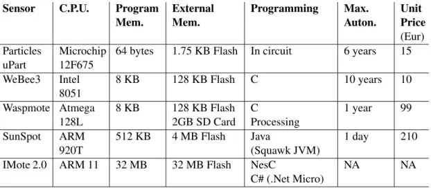
Table 2.1: Characteristics and prices (as of 2010) of five sensor devices
Sensor C.P.U. Program
Mem. External Mem. Programming Max. Auton. Unit Price (Eur) Particles uPart Microchip 12F675
64 bytes 1.75 KB Flash In circuit 6 years 15
WeBee3 Intel 8051 8 KB 128 KB Flash C 10 years 10 Waspmote Atmega 128L 8 KB 128 KB Flash 2GB SD Card C Processing 1 year 99 SunSpot ARM 920T 512 KB 4 MB Flash Java (Squawk JVM) 1 day 210
IMote 2.0 ARM 11 32 MB 32 MB Flash NesC
C# (.Net Micro)
NA NA
tuators [55]. Figure 2.1 illustrates a generic architecture of a sensor device. The dotted lines around some components indicate that they can be replaced. This is not true for the smallest, cheapest node, but is common in the more larger, configurable nodes.
The main concerns in sensor devices are energy autonomy, computational power, size, and cost. These are, naturally, intertangled. Although there have been improvements on sensor hardware and miniaturisation, there is still a long path to run [4, 22]. For example, a device with an increased computational power is tipically less (energy) autonomous.
Many sensor devices have been developed, both academically, and commercially. Five devices representing the current sensor market are described in Table 2.1, in terms of Cen-tral Processing Unit, program memory, external memory, programming model/language, maximum energy autonomy, and unit price (as of 2010). In almost every parameter there is a very significative variance; program memory, for instance, ranges from 64 bytes to 32 MBytes. The table also depicts the correlation between computational power and energy autonomy: nodes with higher computational power deplete their batteries much faster. Table 2.2 summarises the strong points of the considered sensor devices.
Chapter 2. Wireless Sensor Networks 9
Table 2.2: Strong points of five sensor devices
Sensor Evaluation
Particles uPart Very small size (less than 1 cm3, battery included).
WeBee3 Very low price;
Extended battery lifetime.
Waspmote A balanced choice between computational power, battery lifetime, and price;
Modular architecture, allowing to add/remove sensor and communica-tion boards;
Plenty of accessories, including a solar panel that turns the node virtu-ally autonomous;
Commercial support.
SunSpot Computational power.
IMote 2.0 Computational power.
Since there is yet no glimpse of an ideal sensor, it is not possible to dissociate the sensor device from the WSN purpose and, therefore, must choose devices by selecting the desired features at the expense of others.
2.2.1
Nanosensors
Nanotechnology is to become an enabling technology in sensor development. Once ac-complished, nanosensors (sensors in the nanometer scale) will make use of the unique properties of nanomaterials and nanoparticles to detect and measure events in the na-noscale. Nanoactuators, like “normal” actuators, will perform some kind of action on the environment, based on the data provided by the nanosensor nodes. Depending on the nature of the sensing capabilities, nanosensors and nanoactuators can be classified as physical, chemical, or biological [53].
Wireless Nano Sensor Networks (WNSNs) can have environmental, industrial, mili-tary, and biomedical applications. In particular, WNSN can have a large impact in health monitoring systems: sodium, glucose, cholesterol, cancer biomarkers, and other sub-stances may be monitored in blood by means of nanosensors. For instance, nanosensors could monitor the glucose level in blood and transmit the data wirelessly to a cellphone wich, in turn, could forward the data to a healthcare provider [3].
In recent years, many advances have been accomplished in nanotechnology. In Berke-ley, a nanoradio of about ten nanometers in diameter (and several hundred nanometers long) was built and used to perform a FM broadcast across a room [38]. In Harvard, a method for assembling and disassembling nanowires was created [83]. In spite, many more advances must be made before nanosensors can become a reality [3].
As with normal sensors, energy autonomy is a key issue in nanosensors. Although nanomaterials could be used to manufacture nanobatteries with high power density, every
Chapter 2. Wireless Sensor Networks 10
battery needs to be recharged. The concept of self-powered, nano-devices has been re-cently introduced as a solution to overcome the energy autonomy problem. Nanosensors could harvest mechanical (e.g., from human body movements), vibrational (e.g., from acoustic waves), or hydraulic (e.g., blood flow) energy from the environment and convert it into electric energy [3].
2.3
Communication
A typical WSN is a) a wireless ad-hoc network, meaning that there is no preexisting in-frastructure, and b) a multi-hop network, meaning that several nodes may forward a given message from a node to a sink. WSN communication can be characterised in terms of the path in which it takes place: forward and reverse. The former concerns the flow from the sensors to the sink, while the latter concerns the flow from the sink to the sensors. Gener-ally speaking, the reverse path requires higher reliability, because messages may contain code to be deployed, for instance. However, the forward path may also require high relia-bility, specially if some events in the environment must be detected and forwarded to the sink [4].
Transmitting is, arguably, what drains more power from the node’s battery, and, there-fore, what influences most the network lifetime. The approach used to characterise the network lifetime may be based on the first node to wear out its battery, or some other more complex criteria that analyses the network connectivity, regardless of individual nodes with depleted batteries. Power preservation is vital to extend the network lifetime, hence communication protocols must be very efficient [8].
2.3.1
Protocols
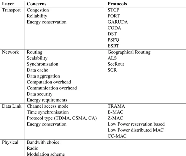
WSN require communication protocols that take into account power conservation and the potentially large number of nodes. Furthermore, the choice, or development, of a protocol is determined by the purpose of the network, or class of networks. Table 2.3 presents the main communication concerns and protocols for WSN, grouped by layer. Further details on the protocols therein can be found in [86].
Not all WSN protocols follow the (traditional) layered approach. Cross-layered proto-cols minimise overhead and can be more energy efficient [84] than their counterparts. In this kind of protocol, the layer interaction varies: SP unifies the Network and Data Link layers, while JOCP unifies all the Transport, Network, Data Link, and Physical layers.
Security Networks can be subject of passive attacks, where there is no traffic modi-fication (e.g., eavesdropping) and active attacks, such as denial-of-service (inhibition of communication), masquerading (access to resources by an attacker pretending to be an authorised user), replay (retransmission of stored messages), and message modification
Chapter 2. Wireless Sensor Networks 11
Table 2.3: Network concerns and protocols for WSN, grouped by network layer
Layer Concerns Protocols
Transport Congestion Reliability Energy conservation STCP PORT GARUDA CODA DST PSFQ ESRT Network Routing Scalability Synchronisation Data cache Data aggregation Computation overhead Communication overhead Data security Energy requirements Geographical Routing ALS SecRout SCR
Data Link Channel access mode Time synchronisation
Protocol type (TDMA, CSMA, CA) Energy conservation
TRAMA B-MAC Z-MAC
Low Power reservation based Low Power distributed MAC CC-MAC
Physical Bandwith choice Radio
Chapter 2. Wireless Sensor Networks 12
Table 2.4: Main standards and technologies for WSN, grouped by network layer
Layers Standards Technologies
Transport Network
Upper layer of Data-Link
ZigBee [87]
WirelessHART [39] Wibree [82]
Lower level of Data-Link Physical
IEEE 802.15.1 [35] IEEE 802.15.3 [36] IEEE 802.15.4 [37]
(new, changed, or re-ordered messages are sent to the network). Some protocols address the security issue: SPINS (Security Protocols for Sensor Networks), for instance, en-sures data confidentiality, two-party data authentication, data freshness, and authenticated broadcast.
2.3.2
Standards and Technologies
Several standards have been proposed for WSN communication. As with protocols, the choice, or development, of a standard is determined by the purpose of the network, or class of networks. Table 2.4 presents some of the WSN standards, technologies, and their relation to the protocol stack.
IEEE 802.15.1 Specifies the physical layer and the medium access control (MAC, lower level of the data-link layer) for Bluetooth communication, where the radio operates at 2.4 GHz.
IEEE 802.15.3 This standard targets real-time, multi-media streaming. It specifies the physical layer and MAC for high data rate for Wireless Personal Area Networks (WPAN). The physical layer operates on a 2.4 GHz radio and supports data rates from 11 to 55 Mbps.
IEEE 802.15.4 Specifies the physical layer and the MAC for low data rate WPAN. The physical layer supports the 868/915 MHz low bands and the 2.4 GHz high band, and MAC uses the CSMA-CA protocol. This standard addresses wireless sensor applications that require short range communication, low energy requirements, and low cost.
ZigBee Builds on IEEE 802.15.4, defining the higher layers of the protocol stack. It is intended to enable networks containing thousands of low cost, low power devices. ZigBee devices are divided into three types: i) coordinators, nodes that initiate network formation and can bridge networks together, ii) routers, that allow multi-hop communication, and
Chapter 2. Wireless Sensor Networks 13
iii) end-devices, sensor or actuator nodes that communicate solely with the routers and coordinators.
WirelessHART This standard targets process measurement and control applications. Like ZigBee, it builds on IEE 802.15.4.
Wibree This technology builds on the IEE 802.15.1 standard, providing low cost and low energy communication for Bluetooth devices.
DASH7 This technology implements the ISO/IEC 18000-7 standard for RFID. By op-erating on the 433 MHz frequency, DASH7 devices have a range of more than 1 Km, use less power, and can transmit through concrete and water. DASH7 does not support streaming, nor synchronisation.
2.3.3
Gathering
Gathering is the process of transmitting data from the sensor nodes to the sink, possibly over multiple hops. In order to achieve extended network lifetime and scalability, this pro-cess must be efficient. Clustering, aggregation, and inference are techniques that improve gathering efficiency by reducing the number of messages on the network.
Clustering protocols, such as LEACH, allow networks to dynamically form clusters in which a head node is responsible for the communication with neighbour clusters). Aggregation protocols use several approaches to limit the number of nodes that a given node is allowed to communicate with. For instance, using PEDAP, the sink node computes routing tables based on the location of the nodes. Whenever a node fails, a new routing table must be computed.
For many applications not all the collected data set is useful. In fact, for applications like temperature monitoring, only a small set of values is necessary, e.g., the maximum and minimum temperatures. Inference is a distributed computing technique that can help reduce the network traffic. For instance, a node could only forward a message if it has a bigger value that the last maximum received, or smaller than the last minimum received.
2.4
Programming Wireless Sensor Networks
Programming WSN is difficult because applications these type of networks are (large-scale) distributed programs that must run on devices that are very limited in terms of hardware and also in terms of energy autonomy [55]. Presently, most sensor nodes run module-based operating systems (e.g., TinyOS [32]) and are programmed in nesC [28] or TinyScript/Mat´e [42]. There are important limitations in this low-level approach [8], namely:
Chapter 2. Wireless Sensor Networks 14
• Lack of a global vision of a sensor network application;
• Absence of a dynamic means of network reprogramming, resulting in the necessity of individual sensor reprogramming, which is unfeasible for large WSN, where massive code deployment is desirable;
• Absence of a rigorous model of the sensor network at the programming level, which would allow for formal verification of program correctness.
Although these limitations are well known and there has been a number of proposals that aim to surpass them, very few WSN rely on higher-level programming models [55].
2.4.1
Operating Systems
A typical WSN operating system provides few abstractions; it supports a programming language, and a low level communication facility. In order to reduce overhead and mem-ory usage, usually only a selection of the operating system modules are deployed to sensor nodes, according to the application needs.
Most current sensor networks run on top of the TinyOS [32] operating system and its sibling programming language nesC [28]. TinyOS provides a very simple, event-based, single-threaded execution-model with non-preemptive tasks. The system is loaded onto the sensor nodes as a set of modules to be used by a target application.
Other operating systems for WSN have been proposed. Contiki [21] is also event-driven, but, unlike TinyOS, supports multi-threaded execution, and dynamic loading of program modules. MANTIS [10], Nano-RK [24], and BTnut [9] operating systems sup-port preemptive multi-threading, meaning that the operating system, not the application programmer, manages the CPU. As a side note, Nano-RK provides control to hardware resources in order to support real-time WSN applications.
There are also systems, such as the Squawk JVM [65] that run directly on the hard-ware, without operating system support. The Squawk JVM supports preemptive multi-threading.
2.4.2
Programming Models and Languages
Traditionally, WSN have been programmed at a very low-level of abstraction, however, there is a growing trend towards the development of high-level programming models and abstractions for these networks. A programming model reflects a given point of view. In the following we present four programming models common in WSN:
• Stream. The programmer sees the network as a data stream, with no perception of the underlying hardware;
Chapter 2. Wireless Sensor Networks 15
• Region. The network can be partitioned into groups of sensors, according to some membership criteria, and programmed on a partition base;
• Database. The network is seen as a dynamic data repository that may be queried by declarative languages such as SQL;
• Computing. The programmer perceives the network as a distributed system that may perform online computation, by hosting autonomous mobile agents, for in-stance.
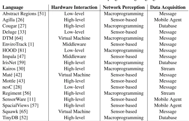
A programming model can be implemented by a programming language in various ways, therefore, it is not sufficient to classify a language. In order to be able to classify the main WSN programming languages, we follow the criteria on [48]. It is based on three items: hardware interaction, network perception, and data acquisition, summarised below. Table 2.5 lists several languages classified according to this criteria.
Hardware Interaction i)Low-level, system-level programming of the sensor networks, where programs make direct calls to the operating system, ii) Virtual Machine, programs run on a software infra-structure that creates an abstraction layer over sensor specific hard-ware and operating system, while allowing the programmer to retain some fine grained control of the applications, iii) Middleware, programming using an API, provided by an underlying middleware, that hides the details of the sensor network from the programmer, and iv) High-level, programming with very high-level abstractions of the network that hide all networking and communication details. Programs are distributed applications that are generally not targeted at a specific sensor network architecture or configuration.
Network Perception i)Macroprogramming, WSN applications are developed as typ-ical distributed applications, without requiring the developer to specify the behaviour of each computing node individually. The low-level details of communication and network architecture are abstracted away, and ii) Sensor-based, WSN applications are developed with the network architecture and, in some cases, with node hardware details in mind.
Data Acquisition i)Communication-centric, lowest level data abstraction where data in the network is seen as messages; ii) Data-centric, high-level data abstractions, namely streams and databases; and iv) Computation-centric, mobile agents evolve to allow com-munication and in-network re-programming.
Generally, high-level languages such as TinyDB [52] are compiled into low-level lan-guages, in the case, nesC [28]. It is rather difficult to ensure that the semantics of the high-level application is equivalent to the semantics of its low-level version. Moreover,
Chapter 2. Wireless Sensor Networks 16
Table 2.5: A classification of WSN programming languages
Language Hardware Interaction Network Perception Data Acquisition
Abstract Regions [51] Low-level Macroprogramming Message
Agilla [26] High-level Sensor-based Mobile Agent
Cougar [27] High-level Macroprogramming Database
Deluge [33] Low-level Sensor-based Message
DTM [64] Virtual Machine Macroprogramming Message
EnviroTrack [1] Middleware Sensor-based Message
HOOD [81] Low-level Macroprogramming Message
Impala [47] Middleware Sensor-based Message
IrisNet [59] High-level Macroprogramming Database
Kairos [30] High-level Macroprogramming Stream
Mat´e [42] Virtual Machine Sensor-based Message
Mottle [43] High-level Sensor-based Message
nesC [28] Low-level Sensor-based Message
Regiment [56] High-level Macroprogramming Stream
SensorWare [11] High-level Sensor-based Mobile Agent
SpacialViews [57] High-level Sensor-based Mobile Agent
Squawk [65] Virtual Machine Sensor-based Message
TinyDB [52] High-level Macroprogramming Database
the low-level programming languages lack a formal specification, making it difficult to reason about program properties.
This situation emerges from the absence of an adequate hardware abstraction, e.g., a virtual machine, that allows a complete formal specification for the semantics of sensor network applications. Some important work has been made in this direction, most notably Mat´e and the Squawk JVM. The problem of lack of specification at the language level is tackled by Callas, a formal-based, type-safe language for WSN that we use along this thesis.
2.5
Research Topics
WSN are a relatively novel subject. While they have drawn a lot of attention in recent years, the constraints imposed by current hardware, communication protocols, and energy autonomy, for example, lead to believe that the subject is to remain under active research. Below, we highlight some research topics. Some concerns, such as energy autonomy, or cost, are transversal to most of the research topics.
Sensor Devices Current sensor devices are very limited. An ideal sensor would be cheap, small, have enough battery to allow its operation for many years, or be able to harvest energy from the environment, have a reasonable computational power, in order to allow the deployment of higher level applications, and would be resilient, in order to allow
Chapter 2. Wireless Sensor Networks 17
large scale deployments from aeroplanes, boats, and other vehicles. Furthermore, for many envisioned applications, sensors must be developed in the micro and nano scale [3, 4].
Communication Protocols and Security Communication protocols must have better performance and energy efficiency, while providing Quality-of-Service. Protocols must also be secure, ensuring that all the stack layers are safe from malicious attacks (current secure protocols address mainly the data-link and network layers) [84].
Programming Abstractions and Correctness Most programming languages for WSN provide few abstractions, whether in terms of language constructs, or in terms of commu-nication [55]. Furthermore, the abstractions are typically not formal based, hence, their correctness is not guaranteed [54].
Fault Tolerance Faults in WSN can be originated by hardware, nodes running out of power, and temporary erroneous readings (transient faults). Currently, the exclusion of nodes with depleted batteries does not obey to time bounds, for example, and there is little support for the detection of erroneous readings [55].
Node Mobility Mobile nodes and sinks have special requirements, such as dynamic net-work topology and delay tolerance, that are not expressed in programming abstractions. Therefore, neighbour discovery and other concerns are dealt with in a per-application basis [55].
Debugging and Testing Debugging and testing WSN is carried out using testbeds and simulators. There is currently no support for debugging and testing at the programming level [55].
Chapter 3
Wireless Sensor Network Simulation
The deployment of WSN poses great challenges. At the node level, the communicational and the computational capabilities are constrained by severe energy and hardware limi-tations. At the network level, the potentially large number of nodes implies that it may be onerous or even unfeasible to test an already deployed network. WSN simulators are computer systems that allow us to deploy and test networks in virtual environments that serve as sandboxes to experiment with communication protocols, radio signal properties, and physical sensing. Therefore, by providing a way of testing and debugging WSN ap-plications in (simulated) environments, simulation can play a decisive role in WSN during testing and deployment.
Another approach towards WSN testing consists of using physical testbeds, such as GNOMES [80], or S-Net [13]. Physical testbeds consist of a set of devices to which sensor nodes are connected in order to be monitored. The gathered data can then be used to infer the network behaviour. Naturally, physical testbeds are not suited for large network testing, because a lot of effort (and hardware) would be required. Some authors note that there has been improvements in mathematical analysis and experimental deployments but, however, simulation is still the preferred tool for the study of WSN [22].
In this Chapter, section 3.1 introduces the topic of WSN simulation and draws a com-parison of popular WSN simulators. Section 3.2 presents the VisualSense WSN simulator, giving some insight into the simulator internals and model definition.
3.1
Wireless Sensor Network Simulators
WSN simulators are complex programs. A simulator should handle large numbers of nodes without degrading performance significantly, model the radio channel, battery dis-charge, physical environment, and support different communication protocols [22]. Ide-ally, it should also provide a graphical interface. Table 3.1 presents the main concerns regarding WSN simulation, grouped by communication protocol support, environment modelling, and graphical support.
Chapter 3. Wireless Sensor Network Simulation 20
Table 3.1: Main concerns in wireless sensor network simulators
Protocol support Environment Modelling Graphical Support
C Classical (e.g., TCP/IP, Ether-net)
B Battery E Edition
A Ad-hoc (e.g., MANET
proto-cols, AODV, DSR)
PP Physical Phenomena A Animation
W Wireless (e.g., propagation, mo-bility, IEEE802.11)
PE Physical Environment D Debugging
WSN Some common WSN Protocols (e.g., Directed Diffusion, S-MAC)
WSN simulators are typically based on discrete event simulation. In this type of sim-ulation, the operation of a system is represented as a chronological sequence of (discrete) events. An event occurs at a given instant in time and sets a new state in the system [1]. The new state may trigger another event, and so on. Discrete event simulation requires a global clock and an event queue to manage the chronological sequence of events. Al-though discrete event simulation can model many systems, it is naturally not suited for every class of system. For instance, physical phenomena and battery discharge requires continuous time simulation. Modelling systems that have discrete and continuous time components is far from trivial.
WSN simulators can be divided into two categories: architecture specific, that model WSN for a given node architecture (e.g., TOSSIM [44], for the Berkeley Motes), and gen-eral simulators, that allow user-defined sensor nodes (e.g.VisualSense [7]). Architecture specific simulators include ATEMU [61], EMStar [29], TOSSIM [44], Avrora [68]. These are not subject of study, since this work aims at a device-independent view of WSN simu-lation. Non specific but also non Open Source simulators include QualNet [77], and OP-NET [25]. These are also not covered here. There are a number of general, Open Source simulators, however, most of them are either abandoned projects (such as JSim [75], Sen-sorSim [60], and Sidh [14]) or do not provide important features such as an advanced GUI and environment modelling. Table 3.2 presents a summary of the features and char-acteristics of general, Open Source simulators, is presented. The characterisation is made against the concerns depicted in Table 3.1.
When choosing a WSN simulator, it is also necessary to assess the project status. In fact, many WSN simulators have been developed, but few remain active projects. An-other important aspect is that node definition is usually done programmatically, thus, the programming language of the node definition API may also be critical. Table 3.3 presents the programming language and project status of the simulators in Table 3.2.
Chapter 3. Wireless Sensor Network Simulation 21
Table 3.2: A characterisation of Open Source, generic WSN simulators
Simulator Protocol
Support
Environment Modelling
Visualisation Additional Notes
JiST/SWANS W/A - A
(Javis/NAM)
OMNET++ C/W/A - E(lim)/A/D
SENS W B/PE
-SENSE W/A/WSN B A
GloMoSim C/W/A/WSN - - Gave origin to a commercial
WSN simulator, QualNet.
ns-2 C/W/A/WSN - A/D
(using nam)
SSFNet C/W/A/WSN - Proprietary
NCTUns C/W/A/WSN - E/A/D
PAWiS C/W/A/WSN B E(lim)/A/D Extends OMNET++
Castalia C/W/A/WSN B/PP/PE E(lim)/A/D Extends OMNET++
J-Sim C/W/A/WSN B/PP/PE E/A/D
VisualSense C/W/A/WSN B/PP/PE E/A/D VisualSense is part of the
Ptolemy II project.
Table 3.3: Project information of Open Source, generic WSN simulators
Language Latest Release Active
JiST/SWANS Java/Jython 1.0.6 (03/2005) Yes, under development.
OMNET++ C++/NED 4.1 (06/2010) Yes, under development.
SENS C++ - (01/2005) No.
SENSE C++ 3.0.3 (04/2008) Yes, maintenance only.
GloMoSim Parsec 2.0 (12/2000) No.
ns-2 C++/OTcl 2.34 (06/2009) Yes. A newer version,
ns-3, is under development.
SSFNet C++/DML/Java 2.0 (01/2004) No.
NCTUns C 6.0 (01/2010) Yes, under development.
PAWiS C++/NED 2.0 (07/2008) No.
Castalia C++/NED 3.0 (08/2010) Yes, under development.
J-Sim Java/Jacl 1.3 (02/2004) No. A patch was released
in 07/2006.
Chapter 3. Wireless Sensor Network Simulation 22 def Counter ( v a l u e ) case operation of g e t : ( c l i e n t ) send v a l u e to c l i e n t i n c r e m e n t : ( )
become new Counter ( v a l u e + 1 )
end case
l e t c = new Counter ( 0 ) i n send i n c r e m e n t to c
Figure 3.1: A counter program written in Simple Actor Language
3.2
The VisualSense Simulator
VisualSense is a modelling and simulation framework for WSN that extends the (actor oriented) Ptolemy II framework [23]. Here, the actor model is briefly presented, focus-ing in the aspects relevant for the understandfocus-ing of VisualSense. Then, the simulator is addressed.
3.2.1
The Actor Model
The actor model is a concurrent computational model proposed by Carl Hewitt [31], and later formalised by Gul Agha [2], where the computational primitives are called actors. An actor executes independently and interacts with other actors solely by asynchronous message passing, therefore, it does not share state.
An actor is defined by a mail address that identifies it, a mail queue that holds the incoming messages, and a behaviour that determines how to handle the messages in the queue and that only accepts a given set of message patterns, thus defining the actor in-terface. Messages that do not comply with the behaviour are ignored. The behaviour maps each accepted message pattern with an operation. While performing an operation, an actor can send messages and create new actors. When the operation is completed, the actor updates its behaviour, whether to a behaviour specified in the operation, or to the same one it previously had, if no replacement was specified in the operation. The newly specified behaviour will be used to handle the next message in the mail queue.
Within an actor system, or configuration, an actor can only send messages to its ac-quaintances: actors whose mail addresses are known to it. Acquaintances may be actors that a given actor knows from its creation (given as parameters), actors that it creates, or actors that it learns of while interacting with other actors. In the actor model, a compu-tation is always triggered by an incoming message. This implies that there must be an external message to boot a given configuration. The actors whose mail address is know outside the configuration are said to be receptionist actors.
Chapter 3. Wireless Sensor Network Simulation 23
Simple Actor Language (SAL) [2], an actor model programming language. TheCounter
behaviour is defined with a parametric acquaintance,value, that is used to hold the counter state. The actor supports two operations:getandincrement. Thegetoperation is triggered by a message with two parameters: the name of the operation to perform,get, and client, the mail address of the requesting actor. Theincrementoperation is triggered by a message with one parameter, precisely the name of the operationincrement. The last two lines in the counter program are not part of the behaviour definition, they serve to create the counter actor, with zero asvalue, and increment it to one.
The get operation executes as one would expect from an asynchronous counter: a message with the current value is sent to the client. The increment operation shows an important aspect of the actor model: the counter becomes another counter, with an updated value, while maintaining its mail address. An actor must always replace its behaviour at the end of an operation, either explicitly, as in theincrementoperation, or implicitly, as in thegetoperation, where abecome selfcommand would be automatically issued.
Although an actor must replace its behaviour after processing a message, it can still maintain a state if the replacement behaviour is always the same and if acquaintances are used to hold the state between replacements. In this example, the acquaintance is a built-in value, while the counter would be an acquaintance of some other actor. The acquaintance relations can be used to achieve actor composition, in the sense that an actor uses other actors as its components.
In the actor model there is unbounded nondeterminism because the arrival order of the messages is arbitrary and the mail queues are unbounded. However, there is also fairness, since all messages are guaranteed to be delivered. This does not mean that a given message will be meaningful when it arrives, since the destination actor may have changed its behaviour in the meantime.
The support for the actor model in programming languages varies in nature. Some languages, such as Clara [19], might be called pure actor languages. Other languages, such as SALSA [71] and Stage [6], extend or modify existing languages (Java and Python, respectively). There are also languages that provide actor libraries, e.g., Scala [58].
The actor model is frequently used in modelling and simulation frameworks. It en-ables composition (using other actors, acquaintances), and encapsulation (message pass-ing is the only form of communication). Therefore, it eases reusability. Besides Ptolemy II, the Simulink [78], LabView [76], and VHDL [79] frameworks are based on the actor model as well.
3.2.2
Ptolemy II
Ptolemy II is an actor-oriented component assembly framework for modelling, simula-tion, and design of concurrent, real-time, and embedded systems [23]. In Ptolemy II, an actor configuration is called a model and is persisted in Modelling Markup Language
Chapter 3. Wireless Sensor Network Simulation 24
Figure 3.2: A Ptolemy II model with atomic actors
(MoML), an XML dialect. The framework has a GUI that allows drag-and-drop model definition, provides access to a library of Ptolemy II actors that perform operations rang-ing from signal analysis to matrix handlrang-ing, and supports loadrang-ing user-defined actors writ-ten in Java.
The two key concepts of the framework are actors and domains. Although commu-nication is asynchronous in the actor model, synchronous interaction can be achieved as a special case of the more general asynchronous interaction. Communication can also be described in terms of being discrete or continuous in nature. In spite of executing independently and not sharing state, actors may share some aspects of their behaviours, particularly in what concerns communication. Ptolemy II captures these different patterns and concerns as domains.
A domain is implemented by a special component called Director that governs the communication between actors. For example, the Discrete Event domain is suitable to simulate digital circuits, where the communication is discrete, while the Continuous Time Model is appropriate to simulate analog circuits, where the communication has a continu-ous nature. The latter is also useful for modelling physical systems that can be described with differential equations.
In the “pure” actor model, the behaviour can be seen as an interface that defines the acceptable message patterns, whereas in Ptolemy II, the actor interface defines both the input and output message patterns, as ports. Also, actors do not interact directly, instead, the connections between them are mediated by relations (a sort of wires for actors) to which the actor ports are linked. In Ptolemy II, actor ports are typed in order to enable type safety. The type system ensures that a port only receives messages of its type, or sub-type. Figure 3.2 presents a Ptolemy II (discrete event) model containing i) aDiscrete Event
Chapter 3. Wireless Sensor Network Simulation 25
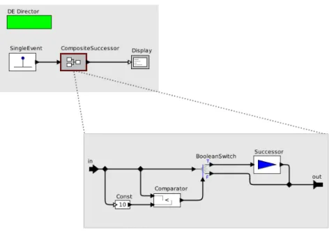
Figure 3.3: A Ptolemy II model with a composite actor
director, ii) aSingle Event actor, configured to send the value “1” at the start of the sim-ulation execution, iii) aSuccessoractor, that adds “1” to every value received, and iv) a
Displayactor, that prints the incoming messages in a GUI window.
A Ptolemy II actor may be atomic, or composite, where an actor contains other actors. In Figure 3.3, theSuccessoractor is replaced by the CompositeSuccessor, that limits the maximum output value to “10”. The notion of actor composition in Ptolemy II is similar, although more restrictive, than the notion of acquaintance in the actor model. In fact, while in the pure actor model acquaintances are used both to connect actors and to com-pose actors, in Ptolemy II acquaintances are established among actors at the same level of hierarchy, but composition is accomplished by composing actors themselves.
Besides reusability and encapsulation, actor composition serves a very important pur-pose: domain heterogeneity. An actor may contain a model that implements another domain. This is useful, for example, to model a sensor that reads some physical value from the surrounding environment. The environment would be modelled using the Con-tinuous Time domain and would be embedded in the Discrete Event where the sensor would be modelled. Ptolemy provides actors that take care of the interaction between the different domains. In more abstract terms, a model is a hierarchical graph where actors are the entities and relations are the arcs. An entity may be either atomic or composite. In the latter case, the entity defines a scope where a domain may be applied.
It is important to distinguish simulated time from simulation time. The former refers to the time interval that is simulated, for instance, ten minutes of a temperature sensing WSN, while the latter refers to the amount of time that it takes for the simulator to perform
Chapter 3. Wireless Sensor Network Simulation 26
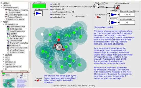
Figure 3.4: A VisualSense network analysis model
the simulation. It may be less than, equal to, or more than the simulated time, depending on the model complexity, the simulator settings, and the hardware platform.
In discrete event simulation, at each simulation clock tick, the events scheduled for that time are triggered (the clock may also “jump” to next queued event). The triggered events will eventually cause the scheduling of other events, simulating the model’s (dis-crete event) behaviour. The Dis(dis-crete Event director handles simultaneous events by deter-ministically adding an index i to the event time-stamp st, obtaining st,i. The simulation
time is therefore two dimensional; the events ea, eb, ec, with time-stamps s1,1, s1,2, s1,3all
occur at t = 1, but in an ordered fashion (first ea, then eb, and finally ec). This ensures
that the simulation execution and results are repeatable.
3.2.3
VisualSense
VisualSense extends Ptolemy II by introducing the Wireless Director (an extension of the Discrete Event Director), that allows for both wired and wireless connections between the nodes. Typically, wireless connections are used among nodes, and wired connections are used inside the nodes, although other configurations are possible.
In the Wireless Domain, rather than directly linked to relations, ports are bounded to Wireless Channels that can simulate radio communication. Wireless Channels are param-eterised in terms of radio signal properties, namely, range, power, propagation speed, loss probability, and propagation factor, that may be overridden by individual ports. When a bounded output port sends a message, the Wireless Channel decides which ports are to receive it, and when, based on the nodes positions, the signal properties, the terrain, and the individual port specifications.
Chapter 3. Wireless Sensor Network Simulation 27
Figure 3.5: A VisualSense sensor node model
VisualSense comes with a library of actors that ease the task of simulation, such as
CollisionDetector, LinkVisualizer,GraphicalLocator, andNodeRandomizer. Figure 3.4 shows a network analysis model. On the upper left corner of the model, there is aWirelessDirector, and aNodeRandomizeractor that distributes, at the start of the simulation, the nodes ran-domly over a given area. At the centre, there is a user defined node called Initiator , that broadcasts the first message. The other nodes around it forward the message, becoming red if they received it directly from the initiator, green if they received it via another node, and staying white if they never receive a message. The model uses two wireless channels:
Channel, for the inter-node communication, andReportChannel, to feed the data analysis actors. Multiple channels can be used to simulate different frequencies, or technologies.
Since VisualSense is a generic WSN simulator, there are no pre-defined sensor node actors. Instead, sensors are modelled from a very high-level, abstract view, using actors. Figure 3.5 shows a model of a node that receives a message on itsin port, prints it on a GUI window (Display), then retrieves the signal properties as a record (GetProperties), extracts only the signal power (RecordDisassembler), scales it according to the antenna area (with aScale actor, renamed toTimes Antenna Area), and, finally, generates a timed plot of the signal power (TimedPlotter).
Regardless of the operation triggered by a received message, the actor performs an-other operation. AClockactor generates periodic events that are used to generate the new position (RampandExpression), of the node in the model (actorSetVariableis configured to set the location attribute of the node).
It is out of the scope of this work to further explore VisualSense’s capabilities in terms of terrain modelling, continuous time modelling, or radio communication. VisualSense is a very powerful simulator. Being generic, it enables to model virtually any sensor node, or WSN, at the cost of having to define the sensor node, the WSN, and the application it runs.
Chapter 4
The Callas Programming Language
Callas [54] is a programming language for WSN, based on the formalism of a process calculus [50, 54], with the goal of establishing a foundation for developing programming languages and run-time systems for sensor networks. Callas may be used as an inter-mediate language upon which high-level programming abstractions may be encoded as semantics preserving, derived constructs. The language offers constructs to describe sen-sor computations, code mobility, and code update.
Callas is type-safe, which means that well-typed (Callas) programs do not produce protocol run-time errors. Language type-safety is of utmost importance in WSN, since it allows premature (static) detection of potential errors, thus minimising the amount of debugging required for an application once it is deployed.
The Callas Virtual Machine (CVM) is a stack-based machine that serves as the run-time system for Callas. The CVM guarantees run-run-time soundness, i.e., that the low-level language (byte-code) it executes preserves the semantics of Callas programs [15].
In Section 4.1, we explain the Callas syntax and semantics along with examples. Sec-tion 4.2 presents an overview of the CVM.
4.1
Programming Language
Section 2.4 classifies programming languages for WSN according to three criteria that can now be applied to Callas. In terms of hardware interaction, Callas falls on the Virtual Machine category, in terms of network perception, it falls on the sensor-based category, and, regarding data acquisition, it is communication-centric.
A Callas program is a sequence of terms whose components are type and module declarations, assignments, expressions, and conditionals. Its syntax is line-oriented, with syntactic terms demarcated by the number of spaces in the beginning of a line (indenta-tion), much like in Python’s programming language.
The Callas syntax and semantics are introduced here by the example of a tempera-ture monitoring application. Figure 4.1 declares three module types that are used in the
Chapter 4. The Callas Programming Language 30 # file: types.caltype defmodule N i l : pass defmodule SenseTemp : N i l sample ( )
N i l g a t h e r (s t r i n g mac , long time , double temp ) defmodule Deploy :
N i l d e p l o y ( SenseTemp senseTemp )
Figure 4.1: Callas type declarations
application. Nil is an empty module type, denoted with keywordpassin its declaration;
SenseTempis a module type with two functions, sample and gather. The former has no parameters and returns a Nil module; the latter receives amacaddress (asstring), a time (as long), and a temp(erature) (as double), returning a Nil module. Finally, the Deploy
module type contains the functiondeploythat receives aSenseTempmodule, and returns a
Nil module.
# file: iface.caltype
from t y p e s import ∗
defmodule Sensor ( Deploy , SenseTemp ) :
N i l l i s t e n ( )
Figure 4.2: A Callas type declaration that serves as a network interface
Type declarations are used to define interfaces. In a Callas network, all nodes share the same (public) interface. This restriction seems plausible because, since nodes collaborate in retransmitting messages from distant nodes to the sink, it is necessary to guarantee, at compile time, that messages sent amongst nodes are always understood. In Figure 4.2, theSensor type declaration extends theDeployandSenseTemptypes, and declares listen, a function with no parameters andNil return.
Although all nodes share the same interface, they may have different behaviors, ac-cording to their role in the WSN. For instance, the sink node in this example application must have a different behaviour from a sensing node because, instead of sensing temper-atures, it must log the readings from rest of the network. The two following sub-sections present a Callas program for the sensing device, and another program for the sink device. The details on the abstract syntax, operational semantics, and type system can be found in [54].
Chapter 4. The Callas Programming Language 31 # file: node.callas from i f a c e import ∗ module m of Sensor : def l i s t e n ( s e l f ) : r e c e i v e def de pl oy ( s e l f , code ) :
extern l o g S t r i n g ( ” Received deployed code . ” )
mem = load
mem = mem | | code
store mem
def g a t h e r ( s e l f , mac , time , temp ) : pass def sample ( s e l f ) : pass store m l i s t e n ( ) every 500 ex pi re 600000 extern l o g S t r i n g ( ” node i s l i s t e n i n g . ” )
Figure 4.3: A Callas program for a sensing node
4.1.1
A Callas Program for a Sensor Node
The Callas code depicted in Figure 4.3 is meant to be deployed in all network nodes, except for the sink. The program starts by importing the (interface) types. Then, it im-plements a module of type Sensor, binding it to variable m. Thereafter, it stores mod-ule m in memory (store m). The language can define timed functions; the expression
listen () every 500 expire 600000sets up a timer that triggers a call to function listen every
500time units for a period of600000 time units. The last expression of the sensor node program calls an external function that logs a message in the sensor’s log file. Theexternal
expression allows for the interaction between Callas programs and sensor internals: the program passes control to the underlying virtual machine and expects a result (in this case the program disregards the result from the call). The type system checks that the external functions are called correctly, i.e., that the node’s native function signatures and return types are observed.
All functions receive, as first parameter, a reference to the module where the call is being made: self. This argument is passed automatically by the run-time system and allows functions to call other functions in its own module, or themselves recursively.
The functions defined in modulem (of type Sensor) are now detailed. Each node is equipped with an incoming and an outgoing queue for interaction with the network. Func-tion listen executes a receiveexpression that explicitly takes a message from the node’s