Controller Design for Neuromuscular Blockade Level
Tracking Based on Optimal Control
Juliana Almeidaa,⇤, Teresa Mendonçab, Paula Rochaa, Luís Rodriguesc
aFaculdade de Engenharia da Universidade do Porto, Rua Dr. Roberto Frias s/n, 4200-465 Porto, Portugal
bFaculdade de Ciências da Universidade do Porto, Rua do Campo Alegre s/n, 4169-007 Porto, Portugal
cDepartment of Electrical and Computer Engineering, Concordia University, 1515 St. Catherine W., Montréal, Québec, Canada H3G 2W1
Abstract
The contribution of this paper is to present and compare two state-feedback design methods for the automatic control of the Neuromuscular Blockade Level (NMB) based on optimal control. For this purpose a parsimoniously parame-terized model is used to describe the patient’s response to a muscle relaxant. Due to clinical restrictions the controller action begins when the patient recov-ers after an initial drug bolus. The NMB control problem, typically consisting of tracking a constant NMB reference level, can be associated with an optimal control problem (OCP) with a positivity constraint in the input signal. Due to the complexity associated with the introduction of a positivity constraint in the input, approximate solutions to this OCP will be found in this paper using two methods. In the first method, the optimal control problem is relaxed into a Semi-Definite Program (SDP) using a change of variables, whereas in the sec-ond method the OCP is approximated by an infinite horizon constrained Linear Quadratic Regulator (LQR) problem. These two controllers are compared with a classical PI controller in simulation. The PI exhibits a slightly worse perfor-mance in terms of the control magnitude but it was not optimized taking this magnitude into account. The simulation results show that the SDP relaxation
⇤Corresponding author
Email address: [email protected] (Juliana Almeida)
CONTROL ENGINEERING PRACTICE Vol. 59 p. 151-158, 2017
DOI: 10.1016/j.conengprac.2016.08.019
and the saturated LQR methods lead to the same controller gains and there-fore the same trajectory tracking using parameters from a patient’s database, thus encouraging its application and validation in clinical trials. Although the performance of the proposed controllers can be compared in terms of how they work when applied to the patient’s database models, the two proposed methods cannot be compared from an optimal control theoretical point of view because they correspond to the solution of two different relaxations of the original control problem using two different functions of merit.
Keywords: Optimal control theory, general anesthesia, neuromuscular blockade level
1. Introduction
State feedback has been widely used to solve a variety of control problems over the last years, including the automatic control of the drug dosing during general anesthesia [1]. The aim of this paper is to present and analyse the per-formance of two state feedback control laws for the administration of a muscle
5
relaxant in order to achieve a desired muscle inactivity (neuromuscular block-ade). At the beginning of the surgery a bolus of muscle relaxant is administered to the patient to facilitate the intubation; after this initial phase the admin-istration of muscle relaxants is maintained to enable the remaining surgical procedures. The effect of the muscle relaxants is measured by the
neuromuscu-10
lar blockade (NMB) level. This level is assessed by applying a supramaximal train-of-four (TOF) stimulus of the adductor pollicis muscle of the patient’s hand and can be registered by electromyography (EMG), mechanomyography (MMG) or acceleromyography (AMG) [2]. The NMB level then corresponds to the first response calibrated by a reference twitch and varies between 100% (full
15
muscle activity) and 0% (full paralysis). According to general clinical practice, the desired NMB level during general surgery is 10%.
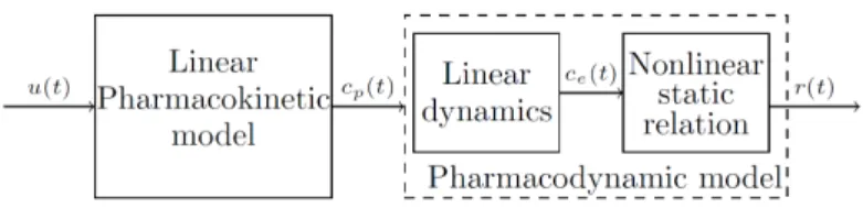
As shown in Fig. 1, the NMB can be modelled by a pharmacokinetic/ pharmacodynamic (PK/PD) model, [3]. This is a physiological model that
Figure 1: PK/PD model diagram scheme.
explains the effect of the muscle relaxant in the patient. The first block relates
20
the drug amount, u(t), with the plasmatic concentration cp(t), through the pharmacokinetic model. The pharmacodynamic model relates the plasmatic concentration with the effect concentration, ce(t), by means of a linear equation, and this is in turn related with the NMB level by a static nonlinearity, known as Hill’s equation, [3]. This model involves a total of eight patient-dependent
25
parameters which may be difficult to estimate.
In this paper an alternative model will be used as basis for the design of our control strategies. This model has been introduced in [4] to overcome the drawback related to the high number of parameters of the PK/PD model. The main advantage of this new model is that it involves a much lower number of
30
patient dependent parameters while keeping an adequate modeling accuracy for control design [5]. For this reason this model is known as parsimoniously parameterized (PP), as shown in [4]. u(t) Linear model ce(t) Static nonlinearity r(t)
Figure 2: PP model diagram scheme.
The PP model is not a physiological model and does not have a PK/PD structure. However it maintains a Wiener structure with the Hill’s equation as
35
nonlinear part, Fig. 2. The PP model has recently been successfully used for the design of some automatic control schemes for drug delivery [6, 7].
con-trollers for the administration of muscle relaxants has been widely addressed in the literature, see for instance [6] and the references therein. However, the
40
optimal control techniques presented here have not been used for solving the tracking problem, which is an important gap in the literature given the optimal nature of the tracking problem. One of the major difficulties preventing the use of optimal control techniques is the positivity constraint in the control input, which corresponds to the amount of drug to be administered, since it is obviously
45
impossible to extract the drug from the blood vessels after its administration, and, also, because in many cases an antidote is not available. Positive control systems, also called non-negative control systems, have been widely studied in the literature but optimal control of positive systems has not been used to ad-dress the NMB tracking problem, to the best of our knowledge. For an earlier
50
account of the properties of positive systems see [8] and for a comprehensive summary of the research on non-negative systems up to 2010 see [9].
In this paper we focus on the feedback control of a positive linear system with a static nonlinearity at the output. Our approach is to formulate an Opti-mal Control Problem (OCP) in order to design a controller that tracks a desired
55
NMB level. This has the advantage of enabling a penalty for the excessive use of drug. An OCP problem with non-negative input and state constraints is in general hard to solve. Reference [10] proposes a technique based on duality for Linear Quadratic Regulator (LQR) problems with constrained input but it assumes that the origin is in the interior of the allowable set for the control
60
inputs, which is not the case for positive systems. In [11] LQ optimal control of positive linear systems is studied. The optimal control is obtained through the solution of a Hamiltonian two point boundary value problem and it is time dependent instead of a state feedback solution. Furthermore, for the contin-uous time example presented in the paper the solution has to be obtained by
65
numerical integration of the equations. A more recent paper on constrained LQR problems [12] proposes to solve the dual problem of the LQR but it yields again a controller that is time dependent that must be computed by a numerical algorithm. An alternative technique for positive linear systems yielding a state
feedback controller is derived in reference [13] where a clamping controller with
70
an integral term of the tracking error is proposed. Although this is an extremely interesting technique leading to a state feedback solution for positive linear sys-tems, it does not correspond to the solution of an optimal control problem. Furthermore, the integral term may suffer from the well known phenomenon of windup, which should be avoided for a drug delivery control problem.
75
There are three important objectives of the work in this paper that are different from the approaches presented in the literature:
• the system has a static nonlinearity at the output,
• integral terms in the controller will be avoided because of possible windup, • the solution that is sought is a feedback controller instead of a time
de-80
pendent control law.
Due to the stated objectives and the added complexity associated with the introduction of a positivity constraint in the input, we consider two different ap-proximations to the solution of an OCP. In the first approximation, the tracking problem is formulated as a suitable finite horizon OCP, which is then relaxed
85
into a semi-definite program (SDP) by replacing the original variables by their moments up to a certain order in the same line of what is done in [14, 15]. The optimal values of the moments can then be computed by semidefinite program-ming solvers [16, 17, 18] and the gains of the state-feedback control law are then computed based on these values. Although the obtained control law is only an
90
approximation of the optimal solution, this approach has the advantage of easily coping with state and input constraints. The second approximation consists of a reformulation of the OCP as an infinite horizon LQR problem with constraints following the ideas presented in [19, 20]. The approximate solution consists of imposing a saturation to the optimal feedback control obtained via the solution
95
of the algebraic Riccati equation associated with the unconstrained LQR prob-lem. As shown in [20] for the discrete-time case, the saturated control law can be optimal for the constrained problem only under certain special conditions,
and therefore such a solution is in general only an approximation to the optimal. Since this method yields an approximate solution of the associated finite
hori-100
zon problem while yielding time independent instead of time dependent gains, it leads to a clear advantage for real-time implementation. These two proposed methods will be compared to a classical PI in the section on simulation results. This paper is organized as follows. Section 2 presents the NMB model used to design the control law and to simulate the patient’s response. Section 3 is
105
dedicated to the design of the state-feedback control laws, and Section 4 presents the main simulation results. Finally, the conclusions are presented in Section 5. 2. NEUROMUSCULAR BLOCKADE MODEL
The PP model for the patient’s NMB level response to the administration of the muscle relaxant rocuronium is presented in this section. This model will
110
be used to design the feedback control laws as well as to simulate the patient’s response.
2.1. Linear block
The linear part of the PP model relates the input signal with the effect concentration, thus grouping the pharmacokinetic process with the linear part
115
of the pharmacodynamic process (of Figure 1). This model can be represented by a third order state-space system [6], as follows:
˙x(t) = 2 6 6 6 4 k3↵ 0 0 k2↵ k2↵ 0 0 k1↵ k1↵ 3 7 7 7 5 | {z } A x(t) + 2 6 6 6 4 k3↵ 0 0 3 7 7 7 5 | {z } B u(t) , ce(t) = h 0 0 1 i | {z } C x(t) (1)
where x(t) = [x1(t) x2(t) x3(t)]T is the state vector, u(t) is the administered muscle relaxant dose, ce(t)is the effect concentration and ↵ > 0 is a
patient-dependent parameter. The positive parameters k1, k2and k3have fixed values,
120
identified in [4], namely k1= 1, k2= 4and k3= 10. 2.2. Nonlinear block
The relationship between the effect concentration and the NMB level is de-scribed by a static nonlinear equation known as Hill’s equation [3]
r(t) = 100
1 +⇣ce(t)
C50
⌘ , (2)
where r(t) is the NMB level and C50= 3.2435is the half maximal effect
con-125
centration. The value of C50 is kept constant for all patients according to the study performed in [21] whereas > 0 is a patient-dependent parameter. 2.3. NMB tracking model
As mentioned before, in this paper a NMB level tracking problem will be considered. For this purpose the system dynamics (1) is written in terms of the
130
variables ˆx(t) = x(t) xe, ˆu(t) = u(t) ueand ˆc
e(t) = ce(t) cee(t), as:
˙ˆx(t) = A ˆx(t) + B ˆu(t) , ˆ
ce(t) = C ˆx(t) (3)
where the matrices A and B are the same as in (1), ue is a constant input value and xe is the corresponding equilibrium value for the state vector, i.e., Axe+ Bue= 0and ce e= C xe. More specifically, xe= [xe1 xe2 xe3] T satisfies 8 > > > < > > > : 10↵xe 1+ 10↵ue = 0 4↵xe 1 4↵xe2 = 0 ↵xe 2 ↵xe3 = 0 , 8 > > > < > > > : xe 1 = ue xe 1 = xe2 xe 2 = xe3 , 8 > > > < > > > : xe= 2 6 6 6 4 1 1 1 3 7 7 7 5u e , (4)
Note that, according to equations (4) and (1), the constant input value ue
135
corresponds to an equilibrium effect concentration ce e= h 0 0 1 i xe given by ce
can be translated into a tracking problem for the associated effect concentration that can be obtained by solving Hill’s equation (2) with respect to ce
eas ce
e= C50(100/re 1)1/ (5)
In terms of system (3), the tracking problem corresponds to tracking a zero
140
reference value for ˆce.
3. FEEDBACK GAIN DESIGN
This section formulates an optimal control problem whose solution will be approximated using two different methods. These two methods will return a state-feedback gain matrix for the administration of the muscle relaxant
rocuro-145
nium with the aim of tracking a desired NMB level.
Given a NMB reference level re, we compute the corresponding effect con-centration reference level ce
e, steady-state input ue and steady state xe. Note that only non-negative values of the state x and the input u make sense for drug administration and therefore one must guarantee that the control input u
150
is non-negative for all time, in which case ueis also non-negative. Since the ma-trix A in (1) is a Metzler mama-trix (i.e, all non-diagonal terms are non-negative) and the input u will be kept non-negative then the state is guaranteed to be non-negative (see [8] for a proof). Consider the optimal control problem with state and input constraints for the controllable and observable system (1):
155 min ˆ u(t),tf J (ˆx(t), ˆu(t)) = 1 2 Z tf t0 ˆ xT(t)Qˆx(t) + ˆuT(t)Rˆu(t) | {z } h(ˆx(t),ˆu(t)) dt s.t. ˙ˆx(t) = A ˆx(t) + B ˆu(t) | {z } f (ˆx(t),ˆu(t)) ˆ x(t0) = ˆx0 (6) ˆ x(tf) = [0 0 0]T ˆ u(t)2 G
with Q = QT > 0and R > 0, ˆx(t) 2 Rnis the state vector, ˆu(t) 2 R is the input signal, t0 is the time instant when the controller action begins (which coincides with the time instant of the patient recovery after an initial bolus), h (ˆx(t), ˆu(t)) and f (ˆx(t), ˆu(t)) are polynomial functions and G is the constrained region for the input values, which is a set defined as
160
G = {ˆu(t) : g (ˆu(t)) 0, 8t 0} ={ˆu(t) 2 R : ˆu(t) + ue 0}
where g (ˆu(t)) is an affine polynomial function. The system dynamics matrices are the same as the matrices presented in Section 2. Note that the final state restriction ˆx(tf) = [0 0 0]T forces the tracking error to be zero at time tf.
The solution to this OCP will now be approximated using two different methods explained in the next subsections.
165
3.1. LMI relaxation
In the first approximation method the OCP is relaxed into a semi-definite program (SDP) by introducing as new variables the moments of the original variables (up to a suitable order) [14, 15]. The transformation of a polynomial OCP into a SDP together with the explanation of how to obtain an approximate
170
optimal control in the form of a feedback law is presented in the sequel. 3.1.1. Semi-definite program
This section follows closely the method proposed in [14, 15]. In order to obtain an approximate solution of the previous OCP, a change of variables is made that transforms this problem into an SDP. For this purpose the new
175
variables are defined as the moments of ¯x = (ˆx , ˆu), i.e., y =
Z T 0
¯
x dt , (7)
To transform a polynomial into a moment we follow a similar procedure to what is done in [14]. To that end, given a polynomial p(¯x) = X
2Nn+1
p ¯x , a linear bounded functional Lis defined as
180
L(p) = X
2Nn+1
p y . (8)
This amounts to replacing the monomials in p by the corresponding integrals, according to (7). Based on the moments y with 2 Bd def= {( 1, . . . , n+1)2 Nn+1:Pn+1
j=1 j d} one also introduces the moment matrix of order d, Md(y), which plays an important role in the reformulation of the OCP (6). The moment matrix has rows and columns labeled by
185
Vd(¯x) = [1, ¯x1, ¯x2, . . . , ¯xn+1, ¯x21, ¯x1x¯2, . . . , ¯x1x¯n+1, ¯xd1, . . . , ¯xdn+1]T (9) and is constructed as
Md(y) = L Vd(¯x) Vd(¯x)T (10) with L as defined in (8). This means that L is applied to each entry of the matrix Vd(¯x) Vd(¯x)T. As a consequence, the cost functional J(ˆx(t), ˆu(t)) can be rewritten as
L(h) = 1 2
X
h y , (11)
where h are the coefficients of the polynomial h (ˆx(t), ˆu(t)) in the OCP
formu-190
lation (6).
To incorporate the system dynamics and the end-point constraints as con-straints of the semi-definite program, monomial test functions (ˆx) are consid-ered. These functions are polynomials given by (ˆx) = ˆx . Note that, on one hand, from the Fundamental Theorem of Calculus:
195
Z T 0
d (ˆx(t))
and on the other hand, using the chain rule and the system dynamics the total time derivative is equal to:
d (ˆx) dt = @ @ ˆx · dˆx dt = @ @ ˆx· f (ˆx(t), u(t)) . (13) Thus for each function (ˆx) one obtains:
Z T 0
@
@ ˆx · f (ˆx(t), ˆu(t)) d t = (ˆxT) (ˆx0) 8 . (14) Since f is a polynomial function of ˆx and ˆu and and @
@ ˆx are polyno-mial functions of ˆx this equation can be rewritten in terms of the moments as
200
P
jaijy↵j = bi, where aij are the coefficients of the moments for i = 1, . . . , M.
The positive integer M represents the number of all possible combinations of the exponents in the polynomial v(ˆx) so that they are not all zero and their sum is less or equal to d. For example, if there are three state variables then v(ˆx) = ˆx 1
1 xˆ22xˆ33 and if d = 2 then all possible combinations such that
205
1+ 2+ 3 d yield M = 9 as will be detailed in section 4.
To handle the state and input constraints the localizing matrix Md(gy)with respect to y and to the polynomial g(ˆu(t)) is defined. This matrix is given by
Md(gy) = L gVd(¯x) Vd(¯x)T , (15) with Vd(¯x)defined in (9). The dimensions of Md(gy)will be such that its entries are moments of order less or equal to d. Therefore, Md(gy)is always of smaller
210
dimension than Md(y). The OCP (6) can then be rewritten as
min y L(h) s.t. X j aijy↵j = bi, i = 1, . . . , M Md(y) 0 (16) Md(gy) 0
This problem is solved using software with an SDP solver such as [16, 17, 18] and the values of the optimal moments y = y⇤ are obtained. Then, a state feedback control input
ˆ u(t) = n X i=1 Kixˆi(t) . (17)
with unknown gains Ki can be determined by replacing (17) in the moments
215
that involve ˆu and recasting it in terms of the moments involving the state. For instance, for a simple system with two state components, ˆx1, ˆx2and one input ˆ
u, the moment y101, where the first index indicates the order of the moment in ˆ
x1, the second index in ˆx2and the third index in ˆu, becomes:
y101= Z T 0 ˆ x1(t)ˆu(t) dt = Z T 0 ˆ x1(t) (K1xˆ1(t) + K2xˆ2(t)) dt = Z T 0 K1xˆ21(t) + K2xˆ1(t)ˆx2(t) dt = K1y200+ K2y110 (18)
Proceeding in the same way for the other moments involving the input yields
220
a system of linear equations. After the values of the optimal moments are obtained the feedback gains can be computed whenever the system of linear equations has a solution.
Remark: Note that two approximations have been made that led to the LMI relaxation when compared to the original problem. First, the considered
225
moment matrix has finite order d. Second, after computing the approximation of order d for the moment matrix we assumed that the control input was a lin-ear state feedback. Therefore, the solution to this problem (i.e., the computed optimal moments and corresponding feedback gain) is only an approximation to the solution of the OCP. As d ! 1 the approximation converges to the optimal
230
solution (under some mild assumptions stated in [14, 15]). Due to this reason, it is necessary to check a-posteriori in simulation if the obtained approximate solution indeed satisfies the original constraints for the set of possible initial
conditions of interest to a given application. Therefore, the theoretical guaran-tees on the input verifying the constraints in the case of the original optimal
235
control problem might be lost in the relaxed solution for a finite d. For linear quadratic problems the hope is that an order d = 2 will be enough based on the LQG problem but there is no guarantee that this is correct when there are constraints on the state and/or on the input.
3.2. Constrained Linear Quadratic Regulator
240
In this section, an infinite horizon linear quadratic OCP with constraints is used to design a state-feedback control law for the NMB level tracking problem. For this purpose consider the following optimal control problem formulation:
min u(t) J (ˆx(t), ˆu(t)) = 1 2 Z 1 t0 ˆ xT(t)Qˆx(t) + ˆuT(t)Rˆu(t) dt s.t. ˙ˆx(t) = A ˆx(t) + B ˆu(t) ˆ x(t0) = ˆx0 (19) ˆ u(t)2 G
where the state ˆx, the input ˆu, the system dynamics, the initial state constraint and G are the same as defined in OCP (6). The optimal solution to this problem
245
will drive the error state ˆx and, consequently, the tracking error (ce cee= ˆx3) to zero asymptotically while respecting the input constraints. The Hamiltonian for this system is
H = inf u2G 1 2 xˆ T(t)Qˆx(t) + ˆuT(t)Rˆu(t) + T(Aˆx + B ˆu) (20)
where = [ 1 2 3]T is the costate. Taking into account that u and R > 0 are scalars, the necessary condition for the minimum in (20) is obtained by
250
Pontryagin Minimum Principle as ˆ u = sat R 1BT = 8 < : 10↵ 1 R , 1 Rue 10↵ ue, otherwise , (21)
To solve for the costate 1 one would need to resort to the costate differential equation and essentially solve a two point boundary value problem that would yield a time dependent control solution instead of a state feedback. Following the ideas presented in [20] for the discrete time case, a suboptimal approximation
255
can be obtained by setting = P0xˆand then ˆ
u(t) = sat (K(t)ˆx(t)) = sat R 1BTP0x(t)ˆ (22) where P0is the unique positive definite solution of the algebraic Riccati equation
Q + ATP + P A P BR 1BTP = 0 (23)
Remark: In a general case for the constrained infinite horizon LQR the proposed saturated state feedback is only an approximate suboptimal solution. Since the infinite horizon was also used as an approximation itself of the finite
260
horizon original problem (6) the proposed saturated state feedback is clearly a suboptimal solution of the original problem. The controller will verify the input constraints due to the saturation but the guarantee of optimality is clearly lost compared to the original optimal control problem. This approximate solution however has the advantage of yielding time independent gains, which are more
265
convenient than time dependent gains for real-time implementations. 4. SIMULATION RESULTS
In order to simulate the performance of the computed feedback control laws a bank R of fifty models Ri with parameters ✓i = (↵i, i) (i = 1, . . . , 50)was considered. These models were obtained by offline identification based on the
270
data collected from fifty patients subject to general anesthesia using rocuronium as a muscle relaxant . The first simulation results use the mean database pa-rameter ¯✓ = (¯↵, ¯) with ¯↵ = 0.0355 and ¯ = 2.716. In all simulations the desired NMB reference level is re= 10.
The control strategy used here can be summarized by the following steps:
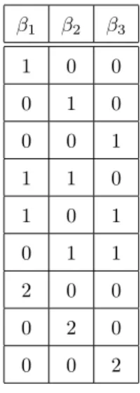
Table 1: Exponents for test function v(ˆx) 1 2 3 1 0 0 0 1 0 0 0 1 1 1 0 1 0 1 0 1 1 2 0 0 0 2 0 0 0 2
• First, a bolus of muscle relaxant of 500µg/kg of rocuronium is adminis-tered, which will be modeled in simulation by an impulse corresponding to an initial condition of x0= 500B, where B is the input matrix; • The patient’s response is monitored to determine the recovery time instant
t0 using the algorithm OLARD [22], which yielded t0 = 29.3 minutes in
280
all simulations;
• After time t0the feedback gain matrix obtained by one of the previously described design methods is used and the state feedback controller is ac-tivated.
4.1. Moment Relaxation
285
For the controller obtained by the moment relaxation from Section 3.1 we considered Q = CTC and R = 1 and we restricted the moment order to be d = 2. The reason why we restricted the moment order d to be equal to 2 was inspired by the fact that if the control problem was not constrained and a Linear Quadratic Gaussian (LQG) output feedback would be used then moments of
290
The test functions were v(ˆx) = ˆx 1
1 xˆ22xˆ33. For moments of order up to d = 2, all possible combinations for the exponents are indicated in table 1. The equality constraint equations corresponding to the entries in table 1, final conditions ˆ
x(tf) = 0and initial conditions ˆx(t0) = eAT500B xe with T = 29.3 minutes
295 are k3↵ (y0001 y1000) + ˆx1(t0) = 0 k2↵ (y1000 y0100) + ˆx2(t0) = 0 k1↵ (y0100 y0010) + ˆx3(t0) = 0 k3↵ (y0101 y1100) + k2↵ (y2000 y1100) + ˆx1(t0)ˆx2(t0) = 0 k3↵ (y0011 y1010) + k1↵ (y1100 y1010) + ˆx1(t0)ˆx3(t0) = 0 k2↵ (y1010 y0110) + k1↵ (y0200 y0110) + ˆx2(t0)ˆx3(t0) = 0 2k3↵ (y1001 y2000) + ˆx21(t0) = 0 2k2↵ (y1100 y0200) + ˆx22(t0) = 0 2k1↵ (y0110 y0020) + ˆx22(t0) = 0
The optimal moment matrix obtained by the solver CVX[18] minimizing y0020+ y0002 subject to the equality constraints and Md(y) 0, Md(gy) 0is
M⇤= Md(y⇤) = 103 2 6 6 6 6 6 6 6 6 6 4 1.3698 0.0126 0.0509 0.0116 0.0079 0.0126 0.0708 0.0909 0.0184 0.0038 0.0509 0.0909 0.1951 0.0184 0.0127 0.0116 0.0184 0.0184 0.0090 0.0007 0.0079 0.0038 0.0127 0.0007 0.0013 3 7 7 7 7 7 7 7 7 7 5 The feedback gains can be computed from the following system of linear equa-tions: 300 2 6 6 6 4 M⇤(2, 5) M⇤(3, 5) M⇤(4, 5) 3 7 7 7 5= 2 6 6 6 4 M⇤(2, 2) M⇤(2, 3) M⇤(2, 4) M⇤(3, 2) M⇤(3, 3) M⇤(3, 4) M⇤(4, 2) M⇤(4, 3) M⇤(4, 4) 3 7 7 7 5 2 6 6 6 4 K1 K2 K3 3 7 7 7 5 (24)
yielding
KLM I = h
0.0312 0.0791 0.3040 i
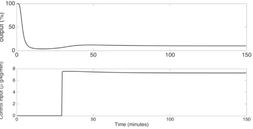
Figure 3 shows the simulation of the NMB level response for the initial conditions x(0) = 500B. Although the values of the the optimal moments will vary when the initial conditions vary, we observed that the controller gains seemed to be very insensitive to variations in initial conditions. As can be seen in Figure
305
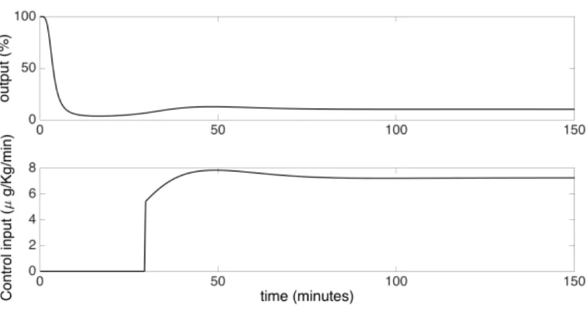
3, the control input u(t) is always non-negative. It can be shown that, due to the structure of the system, this implies that also the state components x = ˆx + xe are non-negative. Therefore, the original problem constraints are indeed satisfied. One can also observe that the NMB level settles to the set-point of 10%.
Figure 3: Simulation of the NMB level response (upper plot) using the state-feedback control (bottom plot) given by the moment relaxation design method.
310
4.2. Constrained LQR
The feedback controller is now obtained using the method of Section 3.2, i.e., by means of a constrained LQR. Using the same weighting matrices as before, i.e., Q = CTC and R = 1, the gain vector obtained for the feedback control law is 315 KLQR= h 0.0312 0.0791 0.3040 i . (25)
This feedback matrix has the same absolute values of the gain obtained for the controller using moment relaxations. The saturated control law is given by
u(t) = sat(KLQRx(t)).ˆ
Since the gains are the same for the LQR and the moment relaxation controllers and the input did not saturate for the simulation of the moment relaxation controller, the two controllers will have the same simulation response for the
320
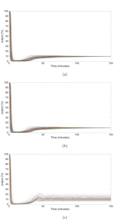
same initial conditions used to produce figure 3. Therefore the response of the LQR controller due of these initial conditions will be omitted. The proposed controllers based on optimal control were also applied to all patient models in the available database and the results are shown in figure 4. From the figure we can see that over the majority of patient models both controllers give a
325
comparable performance.
In the next section both controllers are compared with a classical PI. 4.3. Comparison with Classical PI
In this section we design a PI controller and compare the results with the ones obtained for the LQR and moment relaxation controllers. To design a PI
330
we compute the characteristic polynomial of the closed loop transfer function of the system when ˆu(t) = KPxˆ3(t) KI
Rt
t0x3(⌧ )d⌧ which yields
(s) = s3+ 0.533s2+ (0.0681 0.0018KP)s + 0.0018(1 KI) A simple Routh-Hurwitz approach yields the following conditions for stability
KI < 1 KP < 38 KI 15KP + 19.25 > 0
We chose KP = 1.2, KI = 0.01 and obtained a state trajectory similar to the ones obtained for the case of the LQR and moment relaxation controllers.
335
The simulation results are shown in figure 5. It is clear that the control input respects the positivity constraint.
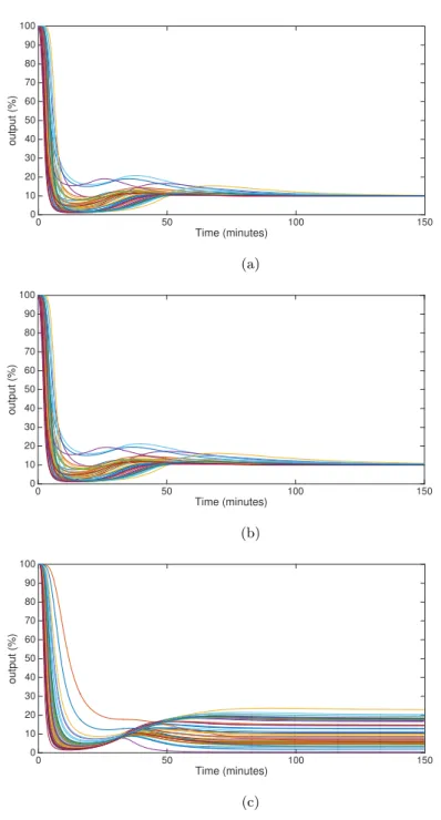
0 50 100 150 Time (minutes) 0 10 20 30 40 50 60 70 80 90 100 output (%) (a) 0 50 100 150 Time (minutes) 0 10 20 30 40 50 60 70 80 90 100 output (%) (b) 0 50 100 150 Time (minutes) 0 10 20 30 40 50 60 70 80 90 100 output (%) (c)
Figure 4: Patient’s NMB level response when the control input is determined by the SDP relaxation method (a), by the constrained LQR (b) and by the PI controller (c) for all cases of the patient database.
Figure 5: Simulation of the NMB level response (upper plot) using the PI control input (bottom plot).
Upon comparison with figure 3 it is also clear that the control signal magni-tude is similar to the one for the simulation of the moment relaxation controller. Figure 4 shows the simulation results for all models in the patient’s database.
340
It is clear that the PI controller does not have a consistent performance for all models as opposed to the moment relaxation and LQR controllers.
Figure 6 shows the performance of the controllers presented above when they are applied to a different model. This model is a physiological model called pharmacokinetic/pharmacodynamic model, [23]. As it is possible to see,
345
the patient responses have the same behavior that the responses presented in Figure 4, which validates the use of these controllers.
5. CONCLUSION
In this paper an optimal control problem was formulated to control the neuromuscular blockade level using a positivity constraint in the control input.
350
Due to the difficulty posed by the posivity constraint, two methods for obtain-ing approximate suboptimal solutions were proposed and compared. The first method consisted of an SDP relaxation leading to Linear Matrix Inequalities (LMIs). The second method consisted of an infinite horizon constrained LQR.
(a)
(b)
(c)
Figure 6: Patient’s NMB level response when the control input is determined by the SDP relaxation method (a), by the constrained LQR (b) and by the PI controller (c) for all cases of the patient database.
For the SPD relaxation, since only moments up to a certain order are
consid-355
ered, the computed feedback gains only correspond to an approximation of the optimal solution of the original problem. For the constrained LQR problem the feedback gain matrix corresponding to a suboptimal solution was obtained using the standard Riccati equation for the unconstrained problem and the control input was defined using a saturation of the optimal feedback control solution.
360
Both methods yield the same gains. The only difference between the solutions of these methods is that the LQR saturates the control input (thus guaranteeing that the positivity constraint is verified) while the moment relaxation solutions does not. The simulation results show that both relaxation methods lead to good tracking using parameters from a patient’s database when compared with
365
a classical PI solution, thus encouraging its application and validation in clinical trials of the proposed methods. Although the performance of the controllers can be compared in terms of how they work when applied to the patient’s database, the two methods cannot be compared from an optimal control theoretical point of view because they correspond to the solution of two different relaxations of
370
the original control problem using two different functions of merit. Finally, in term of computational burden the proposed methods are of comparable cost when the order of the moment relaxation is d = 2. In fact, the moment relax-ation method with input constraints and d = 2 corresponds to solving an LMI for a matrix 6 ⇥ 6 while the LQR synthesis solution corresponds to solving a
375
Riccati equation that can be implemented by an LMI of 5 ⇥ 5. However, the moment relaxation has a larger computational cost than the LQR when the order is d > 2. To the best of the authors’ knowledge it remains to be proved in the literature if d = 2 is the highest relaxation order that one needs to consider to solve a LQR problem even if there are no constraints in the input.
380
Acknowledgements
This work was financially supported by: Project POCI-01-0145-FEDER-006933 - SYSTEC - Research Center for Systems and Technologies - funded by FEDER
funds through COMPETE2020 - Programa Operacional Competitividade e In-ternacionalização (POCI) – and by national funds through FCT - Fundação para
385
a Ciência e a Tecnologia; The author Juliana Almeida acknowledge the support from FCT Fundação para a Ciência e Tecnologia under the SFRH/BD/87128/ 2012. The last author would also like to acknowledge the support of the Natural Sciences and Engineering Research Council of Canada
References
390
[1] T.Mendonça, H.Magalhães, P.Lago, S.Esteves, Hipocrates: A robust sys-tem for the control of neuromuscular blockade, Journal of Clinical Moni-toring and Computer 18 (2004) 265–273.
[2] C.McGranth, J.Hunter, Monitoring of neuromuscular block, Conitinuing Education in Anaesthesia, Critical Care & Pain 6 (1) (2006) 7–12.
395
[3] B.Weatherley, S.Williams, E.Neil, Pharmacokinetics, pharmacodynamics and dose-response relationship of atracurium administered i.v., British Journal of Anesthesia 55 (1983) 39s–45s.
[4] M.M.Silva, T.Wigren, T.Mendonça, Nonlinear identification of a minimal neuromuscular blockade model in anesthesia, IEEE Trans. Contr. Sys.
400
Techn. 20 (1) (2012) 181–188.
[5] M.M.Silva, J.Lemos, A.Coito, B.A.Costa, T.Wigren, T.Mendonça, Local identifiability and sensitivity analysis of neuromuscular blockade and depth of hypnosis models, Computer Methods and Programs in Biomedicine 113 (1) (2014) 23–26.
405
[6] J.Almeida, T.Mendonça, P.Rocha, An improved strategy for neuromuscular blockade control with parameter uncertainty, in: Proc. 50th Conference on Decision and Control (CDC), Orlando, Florida, 2011, pp. 867 – 872.
[7] M.M.Silva, L.PAz, T.Wigren, T.Mendonça, Performance of an adaptive controller for the neuromuscular blockade based on inversion of a wiener
410
model, Asian Journal of Control 17 (2015) 1136 – 1147.
[8] D. Luenberger, Introduction to Dynamic Systems: Theory Models and Applications, John Wiley & Sons, 1979.
[9] W. M. Haddad, V. Chellaboina, Q. Hui, Nonnegative and Compartmental Dynamical Systems, Institute of Aeronautics and Astronautics, 2010.
415
[10] R. Goebel, M. Subbotin, Continuous time linear quadratic regulator with control constraints via convex duality, IEEE Transactions on Automatic Control 52 (2007) 886–892.
[11] C. Beauthier, J. J. Winkin, Lq-optimal control of positive linear systems, Optimal Control Applications and Methods 31 (2010) 547–566.
420
[12] R. S. Burachik, C. Y. Kaya, S. N. Majeed, A duality approach for solv-ing control-constrained linear-quadratic optimal control problems, SIAM Journal Control Optimization 52 (2014) 1423–1456.
[13] B. Roszak, E. J. Davison, The servomechanism problem for unknown siso positive systems via tuning regulators using clamping, in: 2008 IFAC World
425
Congress, Seoul, Korea, 2008, pp. 353 – 358.
[14] J.Lasserre, Moments, Positive Polynomials and Their Applications, 2009. [15] J. B. Lasserre, D. Henrion, C. Prieur, E. Trélat, Nonlinear optimal control
via occupation measures and lmi relaxations, SIAM Journal on Control and Optimization 47 (2008) 1643–1666.
430
[16] J.F.Sturm, Sedumi: a linear/ quadratic/ semidefinite solver for Matlab and Octave, 2013.
[17] J.Lofberg, Yalmip: A toolbox for modeling and optimization in matlab, 2013.
435
URL http://users.isy.liu.se/johanl/yalmip/
[18] M. C. Grant, S. P. Boyd, The cvx users’ guide release 2.1, Tech. rep., CVX Research, Inc.
[19] R. Bellman, Dynamic programming and a new formalism in the calculus of variations, Proceedings of the National Academy of Sciences of the United
440
States of America 40 (1) (1954) 231–235.
[20] J. D. Doná, M. Seron, D. Mayne, G. Goodwin, Enlarged terminal sets guaranteeing stability of receding horizon control, Systems Control Letters 47 (2002) 57–63.
[21] H.Alonso, T.Mendonça, P.Rocha, A hybrid method for parameter
estima-445
tion and its application to biomedical systems, Computer Methods and Programs in Biomedicine 89 (2008) 112–122.
[22] M.M.Silva, C.Sousa, R.Sebastião, T.Mendonça, P.Rocha, S.Esteves, Total mass tci driven by parametric estimation, in: Proc. 17th Mediterranean Conference on Control and Automation, Thessaloniki, Greece, 2009, pp.
450
1149–1154.
[23] J. M. Bailey, W. M. Haddad, Drug dosing control in clinical pharmacology, Control Systems Magazine, IEEE 25 (2) (2005) 35–51.