Parametric imaging of FET PET using nonlinear based fitting

2016

UNIVERSIDADE DE LISBOA

FACULDADE DE CIÊNCIAS

DEPARTAMENTO DE FÍSICA

Parametric Imaging of FET PET using Nonlinear based

Fitting

Inês Isabel Monteiro Costa

Mestrado Integrado em Engenharia Biomédica e Biofísica

Perfil de Sinais e Imagens Médicas

Dissertação orientada por:

Professor Dr. Pedro Miguel Dinis de Almeida

Dr. Christoph Lerche

i

Acknowledgments

First I acknowledge my external supervisor Dr. Christoph Lerche of the INM-4 at Forschungzentrum Jülich for his teachings and guidance − and unlimited patience for all my questions, and fitting procedure struggles. I also acknowledge my internal supervisor, Dr. Pedro Almeida of the Faculdade de Ciências da Universidade de Lisboa for his supervision, and for helping me getting the opportunity to develop this work.

I would like to thank Dr. Liliana Caldeira of the INM-4 at Forschungzentrum Jülich for welcoming me there for the first time three years ago (when it all started!), and once again this time. Her help was of upmost importance on both occasions, on both academic and personal levels.

I would like to show my gratitude to all the members of the PET Group of INM-4 at Forschungzentrum Jülich. I was incredibly lucky to be working with such a great group of people, and with whom I learned so much. They were the most supportive working group I could have asked for, and kind enough to forgive me every time I swapped having lunch with them for a run around the center. I would like to thank the extraordinary group of people I met while living in Aachen. They were many, from all around the world, and all of them contributed to make this past year an unforgettable experience. However, special thanks goes to Klim, Ilya, Deep, and Felix, who were the coolest flatmates ever, Borjana, and Yannick. I owe you all a lifetime supply of pastéis de nata.

Finally, I must express my very profound gratitude to my family. They were the ones who always believed. No matter where I am, I will always carry them in my heart; no matter who I become, I know they will always support me. This accomplishment would not have been possible without them. Thank you.

ii

Summary

The importance of radiolabeled amino acids in Positron Emission Tomography (PET) imaging of the brain has been demonstrated by several studies. The most well studied amino acid tracer is 11 C-metionine, but because of the short half-life of 11_C, 18_{F-labeled amino acid analogues have been} developed for tumour imaging. A number of studies have proven the importance of O-(2-18 F-Fluoroethyl)-L-tyrosine (FET) in determining the extent of cerebral gliomas, biopsy guidance, treatment planning, and detecting recurrence of brain tumours. It was also demonstrated that dynamic changes of FET accumulation in gliomas are variable. High-grade gliomas (HGG) are characterized by an early peak, followed by decrease of FET uptake, whereas the uptake in low-grade gliomas (LGG) steadily increases.

Eleven patients (3 female, 8 male, age: 45±15 years) with untreated primary brain tumours and histopathologic confirmation were studied. Six patients had HGG, while the remaining 5 were diagnosed with LGG. PET acquisition was done with the PET Insert of a hybrid Siemens 3T MR-BrainPET system. For tumour volume fitting, a segmentation procedure was applied. After segmentation, the mean time-activity curve (TAC) of the segmented tumour volumes (STVs) was calculated. Linear and nonlinear regression were used to fit to the TAC of each volume. When performing the fits with the linear model, the first 5 minutes of acquisition were discarded. For the nonlinear regression, the fits were applied to the mean TAC from 2 to 60 minutes after injection. Parametric images were calculated based on nonlinear regression fitting of FET data in each voxel. Three different nonlinear models were tested: an exponentially damped linear model, an exponentially damped linear model with an offset, and an exponentially damped linear model with square-root time dependence. The considered nonlinear model parameters were amplitude, A, and κ. The parametric images of manually selected tridimensional volumes containing the tumour were generated. Linear regression based parametric images were also computed for comparison, and the assessed parameters were intercept and slope. Whole-head parametric images were calculated based on nonlinear regression fitting using the exponentially damped linear model with square-root time dependence.

Nonlinear regression models were more accurate at reproducing FET TAC characteristics. The most robust models are the exponentially damped linear models without offset. For mean TAC fitting, a model with square-root time dependence reproduced FET activity curves more accurately, with coefficient of determination (𝑅2_{) values between 0.94 and 1.00. The A parameter from the exponentially}

damped linear model with square-root time dependence was the only one significantly different between HGG and LGG (p-value= 0.04, α=0.05). When generating parametric images based on voxel-wise fit, the nonlinear regression models with 2 parameters performed the best, with 𝑅2 _{close to 1. Visual}

distinction between tumour grades was possible by comparing the amplitude images with the images of the summed activity across time. In the amplitude, LGGs take values similar to the ones of the surrounding background, thus disappearing from the image. On the other hand, HGGs amplitude images reproduce tumour uptake. Linear regression model fits returned 𝑅2 _{values that were close to zero in both}

mean TAC fitting, and parametric image calculation. Grade distinction was possible based on the slope parameter alone, with LGGs showing higher slope values than the neighbouring tissue, and HGGs showing lower slope values than their surroundings. In general, though nonlinear models reproduce FET time activity curves more accurately, the distinction between low-grade and high-grade tumours based on one parameter only is better achieved by using linear regression model fitting. However, a reliable differentiation seems to be possible with joint analysis of A and κ parametric images.

iii

Resumo

A importância do uso de aminoácidos marcados com isótopos radioativos em estudos de Tomografia de Emissão de Positrões (PET) tem sido amplamente demonstrada. Dentro deste grupo de traçadores, a metionina marcada com 11_{C tem sido o mais estudado. No entanto, a curta semi-vida do} radioisótopo 11_{C tem levado ao desenvolvimento de marcadores análogos. Os marcadores com o} radioisótopo 18_{F revelam-se os mais promissores para deteção de tumores no cérebro. Mais} especificamente, o marcador O-(2-18_{F-Fluoroetil)-L-tirosina (FET) provou ser de grande importância na} determinação da dimensão de tumores cerebrais e dos locais onde realizar a biopsia, no planeamento do tratamento a aplicar, e na deteção de recorrências. Foi também demonstrado que a forma como o FET é metabolizado ao longo do tempo depende do grau do tumor em estudo. Em gliomas de alto grau (HGG), a taxa de captação do FET é caracterizada por um pico inicial, seguido de uma diminuição da captação de FET, enquanto que em gliomas de baixo-grau (LGG) a taxa de captação do marcador tem um aumento contínuo ao longo do tempo.

O presente estudo contou com 11 pacientes (3 mulheres, 8 homens, idade: 45 ± 15 anos) com tumores cerebrais primários não tratados confirmados por histologia. Seis pacientes foram diagnosticados com HGG, enquanto os restantes 5 foram diagnosticados com LGG. Os dados de PET foram adquiridos com o PET Insert do sistema híbrido Siemens 3T MR-BrainPET. As imagens foram segmentadas de forma a extrair apenas o volume correspondente ao tumor. Após a segmentação, calculou-se a média das curvas de tempo-atividade (TAC) dos volumes tumorais segmentados (STVs), e foram usados métodos de regressão linear e não linear para fazer o ajuste à TAC de cada volume. Para calcular os ajustes com o modelo linear, foram descartados os primeiros 5 minutos de aquisição. Os ajustes baseados na regressão não-linear foram aplicados à TAC correspondente à média entre os 2 e os 60 minutos de aquisição após a injeção. As imagens dos parâmetros foram calculadas a partir dos ajustes baseados na regressão não linear e aplicados a cada voxel. Foram testados três modelos não lineares diferentes: um modelo linear amortecido exponencialmente, um modelo linear amortecido exponencialmente e com um offset, e um modelo linear amortecido exponencialmente com o tempo dependente da raiz quadrada. Dos ajustes não lineares, foram extraídos dois parâmetros: a amplitude, A, e o parâmetro κ. De seguida, geraram-se as imagens dos parâmetros calculados sobre uma área tridimensional selecionada manualmente e contendo o tumor. Para tal, além dos três modelos não lineares, utilizou-se também o modelo linear, de modo a permitir uma comparação entre os diferentes métodos. No caso dos ajustes lineares, os parâmetros extraídos foram a ordenada na origem e o declive. Calcularam-se também as imagens dos parâmetros da regressão não linear usando o modelo linear amortecido exponencialmente com o tempo dependente da raiz quadrada para a cabeça inteira.

Os modelos não-lineares foram mais precisos na reprodução das curvas de FET. Os modelos mais robustos foram os modelos lineares exponencialmente amortecidos sem offset. Nos ajustes aplicados à TAC média dos STVs, o modelo linear amortecido exponencialmente com o tempo dependente da raiz quadrada provou ser o que reproduz mais precisamente os dados, com valores de 𝑅2

entre 0,94 e 1,00. O parâmetro A do modelo linear amortecido exponencialmente com o tempo dependente da raiz quadrada foi o único que revelou uma diferença significativa entre HGG e LGG (p-value= 0.04, α=0.05). Ao gerar imagens paramétricas com base nos ajustes aplicados a cada voxel, os modelos de regressão não-linear com 2 parâmetros tiveram o melhor desempenho, com valores de 𝑅2 perto de 1. Combinando as imagens do parâmetro amplitude e as imagens da atividade total ao longo do tempo, foi possível distinguir entre graus tumorais. Os LGGs assumem valores de amplitude próximos dos valores do tecido saudável à sua volta, e por isso “desaparecem” da imagem paramétrica da amplitude. No caso dos HGGs, a imagem da amplitude reproduz a atividade no tumor. Os ajustes realizados com base na regressão linear devolveram valores de 𝑅2 próximos de zero, quer no caso dos

iv

STVs, quer no cálculo das imagens paramétricas. A distinção entre HGG e LGG é possível com base nas imagens paramétricas do declive, com os LGGs a assumirem valores de declive superiores aos do tecido saudável adjacente. Com os HGGs, a situação é a oposta: os valores do declive no tumor são inferiores aos do tecido saudável que o rodeia. Em geral, os modelos não lineares reproduzem melhor os dados provenientes de FET PET, mas a distinção entre HGG e LGG baseada num parâmetro apenas é melhor conseguida através de regressão linear. No entanto, a distinção entre HGG e LGG também é possível analisando simultaneamente as imagens dos parâmetros A e κ.

v

Index

Acknowledgments ... i

Summary... ii

Resumo ... iii

List of figures ... vii

List of tables ... x

List of abreviations ... xi

1. Introduction ... 1

1.1. PET tracers in Brain Imaging ... 1

1.1.1. FDG ... 1

1.1.2. FET ... 2

1.1.3. Other tracers ... 3

1.2. Tracer kinetic modelling... 4

1.2.1. Compartmental modelling ... 4

1.2.2. Graphical analysis ... 6

1.2.3. Other modelling approaches ... 8

1.3. Parametric Imaging in PET ... 8

1.4. Brain tumour types and grades ... 10

1.4.1. Low-grade Gliomas ... 10

1.4.2. High-grade Gliomas ... 11

1.5. Imaging of Brain Tumours ... 12

1.5.1. Comparison between FET PET and FDG PET ... 12

1.5.2. Comparison between FET PET and MRI ... 13

1.5.3. FET PET in brain imaging ... 15

1.6. Motivation ... 17

2. Methods ... 19

2.1. Patients ... 19

2.2. Data acquisition, reconstruction, and motion correction ... 19

2.3. Tumour segmentation ... 20

2.4. Linear model ... 21

2.5. Empirical nonlinear models ... 21

2.6. Fitting of Tumour TAC ... 23

2.7. Parametric images ... 24

3. Results ... 26

vi

3.2. Tumour region parametric images ... 37

3.2.1. Linear model ... 37

3.2.2. Nonlinear models... 38

3.3. Whole-head parametric images ... 45

4. Discussion ... 47

4.1. Fits applied to segmented tumour volume ... 47

4.1. Voxel-wise fit and parametric images ... 49

4.2. Whole-head parametric images ... 50

5. Conclusion ... 51

References ... 52

Appendix I - Mathematica Package for Reading ECAT7 files ... 55

Appendix II - Source code for segmentation and STV fitting ... 60

vii

List of figures

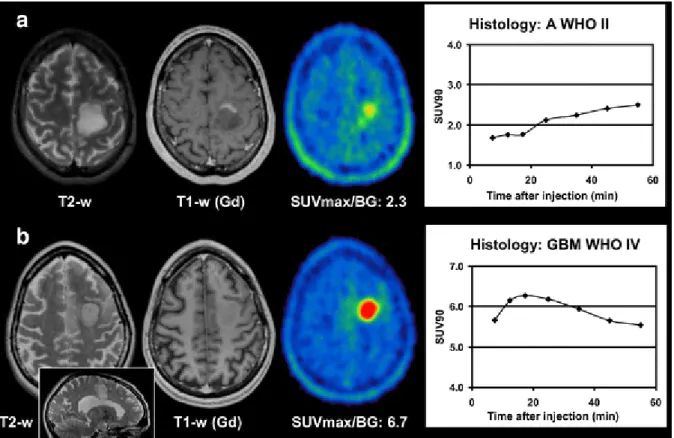
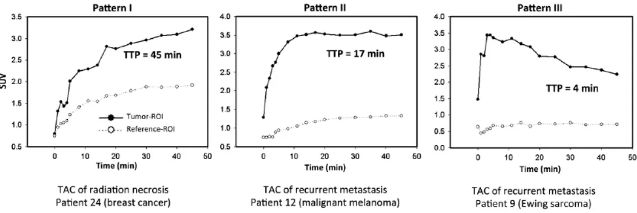
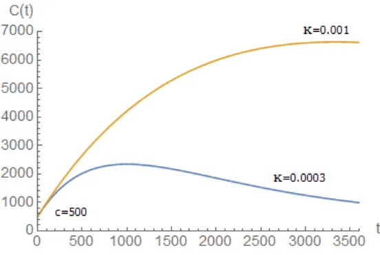
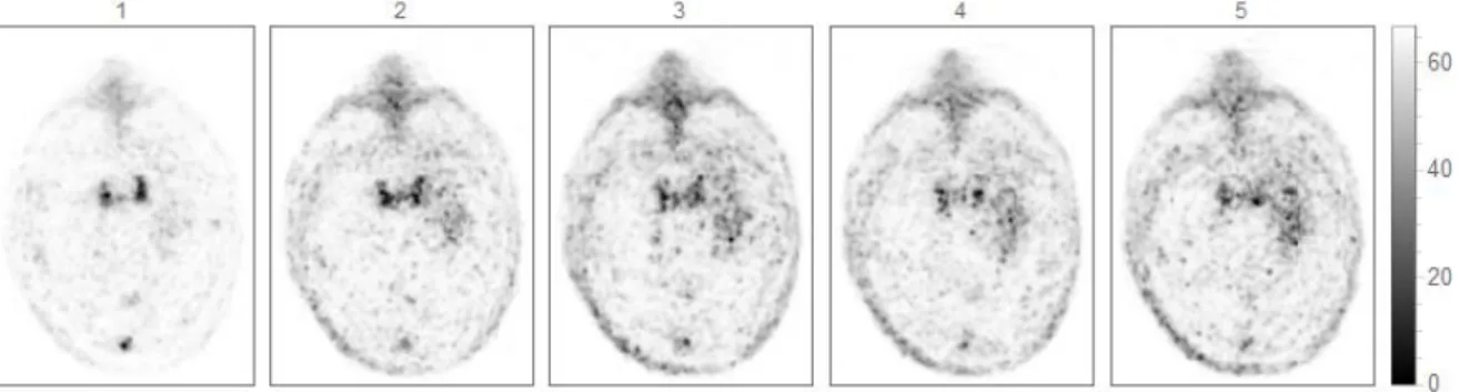
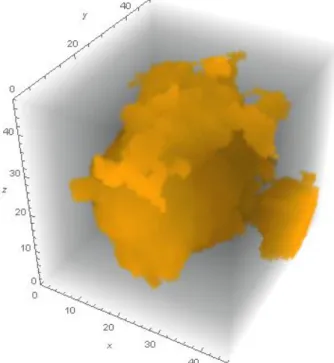
Figure 1.1 - Chemical structure of the FET tracer (adapted from [9]). ... 2 Figure 1.2 - High-grade glioma in the frontal lobe. (A) FDG PET. (B) FET PET. Delineation of the tumour is difficult on FDG images, while FET depicts the solid tumour mass and indicates an optimal biopsy site [13]. ... 3 Figure 1.3 - Steps for developing a model [21]. ... 6 Figure 1.4 - Logan plot. The input is shown on the left, and the output is shown on the right (adapted from [33]). ... 7 Figure 1.5 - Schematic representation of the methods used for parametric estimation (adapted from [38]). ... 9 Figure 1.6 - Histologic criteria of the WHO for the classification of gliomas. (A) Fibrillary astrocytoma is characterized by increased cellularity. (B) Anaplastic astrocytoma is characterized by nuclear atypia and mitoses. (C) Glioblastoma multiform is characterized by necrosis with cells arranged around the edge of the necrotic tissue (adapted from [40]). ... 10 Figure 1.7 - Examples of a) low-grade tumour and b) high-grade tumour. Both studies show circumscribed hypertense lesions in T2-weighted MRI with pathologic contrast enhancement. In the low-grade tumour, some of the regions show contrast enhancement in T1-weighted MRI. MR diagnosis was pseudotumoral multiple sclerosis plaque in b), due to the irradiation of the corpus callosum, shown in the inset sagittal view. Dynamic evaluation shows increasing SUV90 values until the end of acquisition. On the other hand, for the high-grade tumour, dynamic evaluation shows an early peak with decreasing SUV90 values until the end of acquisition (adapted from [53])... 16 Figure 1.8 - Examples of kinetics of radiation necrosis (pattern I) and recurrent brain metastasis (patterns II and III). Dynamic evaluation of patient 24 shows constantly increasing FET uptake until the end of acquisition. Dynamic evaluation of patient 12 shows early peak of FET uptake, followed by stable uptake until end of acquisition. Dynamic evaluation of patient 9 shows early peak of FET uptake followed by constant decline of uptake until end of acquisition. (adapted from [56]). ... 18 Figure 2.1 - FET PET Workflow. ... 20 Figure 2.2 - Exponentially damped linear model with low κ value (blue line) and high κ value (orange line). ... 22 Figure 2.3 - Exponentially damped linear model with an offset plotted with and low κ value (blue line), and high κ value (orange line), for an offset c=500. ... 23 Figure 2.4 - Exponentially damped model with square-root time dependence: model behaviour with low κ value (blue line), and high κ value (orange line). ... 23 Figure 2.5 - First 5 frames of a dynamic FET PET scan (one minute each). ... 24 Figure 3.1 - 3D mask used for HG020 segmentation. ... 26 Figure 3.2 - Fits applied to mean TAC of STV for HG020. A) Linear model; B) Exponentially damped linear model with square root time dependence. ... 26 Figure 3.3 - 3D mask used for HG021 segmentation. ... 27 Figure 3.4 - Fits applied to mean TAC of STV for HG021. A) Linear model; B) Exponentially damped linear model with square root time dependence. ... 27 Figure 3.5 - 3D mask used for LG090 segmentation... 28 Figure 3.6 - Fits applied to mean TAC of STV for LG090. A) Linear model; B) Exponentially damped linear model with square root time dependence. ... 28 Figure 3.7 - 3D mask used for LG131 segmentation... 28 Figure 3.8 - Fits applied to mean TAC of STV for LG131. A) Linear model; B) Exponentially damped linear model with square root time dependence. ... 29

viii

Figure 3.9 - 3D mask used for LG247 segmentation... 29 Figure 3.10 - Fits applied to mean TAC of STV for LG247. A) Linear model; B) Exponentially damped linear model with square root time dependence. ... 30 Figure 3.11 - 3D mask used for HG417 segmentation. ... 30 Figure 3.12 - Fits applied to mean TAC of STV for HG417. A) Linear model; B) Exponentially damped linear model with square root time dependence. ... 30 Figure 3.13 - 3D mask used for LG465 segmentation. ... 31 Figure 3.14 - Fits applied to mean TAC of STV for LG465. A) Linear model; B) Exponentially damped linear model with square root time dependence. ... 31 Figure 3.15 - 3D mask used for HG469 segmentation. ... 32 Figure 3.16 - Fits applied to mean TAC of STV for HG469. A) Linear model; B) Exponentially damped linear model with square root time dependence. ... 32 Figure 3.17 - 3D mask used for HG512 segmentation. ... 32 Figure 3.18 - Fits applied to mean TAC of STV for HG512. A) Linear model; B) Exponentially damped linear model with square root time dependence. ... 33 Figure 3.19 - 3D mask used for HG552 segmentation. ... 33 Figure 3.20 - Fits applied to mean TAC of STV for HG552. A) Linear model; B) Exponentially damped linear model with square root time dependence. ... 34 Figure 3.21 - 3D mask used for HG598 segmentation. ... 34 Figure 3.22 - Fits applied to mean TAC of STV for HG598. A) Linear model; B) Exponentially damped linear model with square root time dependence. ... 35 Figure 3.23 - Comparison between the nonlinear models used to calculate the parametric images of HG021 and LG131 when applied to the mean SUVs of the respective STVs across time. The first row shows the results from the nonlinear regression fit with the simple exponentially damped linear model (A and B). The second row shows the results obtained with the exponentially damped model with an offset (C and D), and the last row shows the results from the exponentially damped linear model with square-root time dependence fit (E and F). ... 36 Figure 3.24 - Parametric images of slope and intercept from linear regression fitting of data in each voxel. ... 38 Figure 3.25 - Parametric images of A and κ obtained from nonlinear regression fitting of data in each voxel (exponentially damped linear model). ... 38 Figure 3.26 - Parametric images of A and κ obtained from nonlinear regression fitting of data in each voxel (exponentially damped linear model with offset)... 39 Figure 3.27 - Parametric images of A and κ obtained from nonlinear regression fitting of data in each voxel (exponentially damped model with square-root time dependence). ... 39 Figure 3.28 - Fit results of the three nonlinear models on a single voxel inside the tumour region (top plot, on the left) and on the STV (bottom plot, on the left) of patient LG131, and respective parametric images (on the right). (A) shows the results from the nonlinear regression fit with the simple exponentially damped linear model. (B) shows the results obtained with the exponentially damped model with an offset, and (C) shows the results from the exponentially damped linear model with square-root time dependence fit. ... 40

Figure 3.29 - Parameter distribution obtained from fitting of LG131 tumour and control data in each voxel: a) exponentially damped linear model; b) exponentially damped linear model with square-root time dependence; c) linear model. ... 41

Figure 3.30 - Parameter error histograms obtained from fitting of LG131 data in each voxel: a) exponentially damped linear model; b) exponentially damped linear model with time dependence; c) linear model. ... 42

ix

Figure 3.31 - Parameter distribution obtained from fitting of HG021 tumour and control data in each voxel: a) exponentially damped linear model; b) exponentially damped linear model with time dependence; c) linear model. ... 43 Figure 3.32 - Parameter error histograms obtained from fitting of HG021 data in each voxel: a) exponentially damped linear model; b) exponentially damped linear model with time dependence; c) linear model. ... 44 Figure 3.33 - Parameter error histograms obtained from fitting of LG131 data in each voxel with the exponentially damped linear model with an offset. ... 44 Figure 3.34 - Whole-head parametric images of A and κ obtained from nonlinear regression with exponentially damped linear model with square-root time dependence fitting of data in each voxel. ... 46

x

List of tables

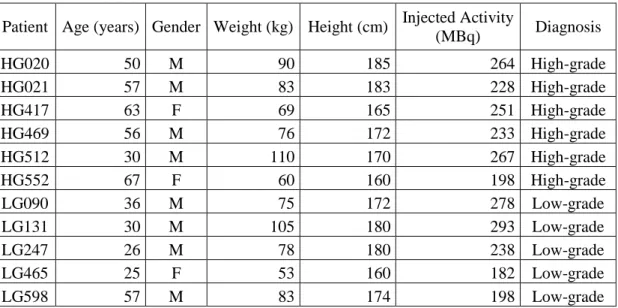
Table 2.1 - Individual patient data including age, gender, weight, height, injected activity, and diagnosis after stereotactic byopsy. ... 19 Table 2.2 - Estimated segmentation thresholds. ... 21 Table 3.1 - Summary of the estimated parameters from linear and nonlinear regression model fit to the STVs. ... 35 Table 3.2 - Mean values of the intercept parameter from linear regression model fit to the STVs. ... 36

Table 3.3 - Mean values of the slope parameter from linear regression model fit to the STVs. ... 37

Table 3.4 - Mean values of the amplitude (A) parameter from nonlinear regression model fit to the STVs with the exponentially damped linear model with square-root time dependence... 37 Table 3.5 - Mean values of the κ parameter from nonlinear regression model fit to the STVs with the exponentially damped linear model with square-root time dependence. ... 37 Table 3.6 - Mean R2 _{from the voxel-wise fit with the linear and the non-linear models. ... 45}

xi

List of abreviations

BBB Blood-Brain Barrier

CT Computed Tomography

FDG 18_{F-Fluorodeoxyglucose}

FDOPA L-3,4-Dihydroxy-6-18_{F-fluorophenylalanine} FET O-(2-18_{F-Fluoroethyl)- L-tyrosine}

FMISO 18_{F-Fluoromisonidazole} HG(G) High-grade (Glioma) LG(G) Low-grade (Glioma) MET 11_C-Methionine

MRI Magnetic Resonance Imaging PET Positron Emission Tomography ROC Receiver Operating Characteristic ROI Region of Interest

STV Segmented Tumour Volume

SUV Standard Uptake Value TAC Time-activity Curve TBR Tumour-to-Brain Ratio

TTP Time-to-Peak

1

1. Introduction

1.1. PET tracers in Brain Imaging

The first step in a Positron Emission Tomography (PET) study is the production of the radiopharmaceutical. Development of specifically targeted radiopharmaceutical enables us to study the biochemistry of the brain due to the very high sensitivity of this imaging method. The ability to study biomolecules at a nanomolar to picomolar concentration in vivo allows a systematic study of various physiological processes. These advancements in imaging technology have further enhanced our capability to study the various processes in small brain regions.

Metabolic studies using 18_{F-fluorodeoxyglucose (FDG), various amino acids such as} 11 C-methionine (MET) and O-(2-18_{F-Fluoroethyl)- L-tyrosine (FET), and perfusion studies with} 15_O-labelled molecules have now been carried out for a number of years. Neurochemical processes in the brain are the primary targets for many new radiopharmaceuticals. There are numerous neurochemical pathways in the brain, and each one comprises a large number of proteins that are involved in health and disease. Once the radiopharmaceutical is available, it is introduced into the patient's body, usually by injection. The time between the administration of the radiopharmaceutical and the beginning of data acquisition depends on the purpose of the imaging study and the nature of the tracer. Data acquisition takes place with the patient laying still in a bed. The radioactive isotope with which the radiopharmaceutical has been labelled emits gamma rays as a product of radioactive decay. As the gamma rays emanate from the patient, they are detected and recorded by imaging hardware. Positional and directional information about each gamma ray are measured, and the results are tailed into a histogram of discrete position-direction bins. The resulting histogram bins contain measurements of the projections. The projection data is then used to estimate the desired tomographic images. The final step is image analysis.

1.1.1. FDG

The phosphorylation of glucose, an initial and important step in cellular metabolism, is catalyzed by hexokinases (HKs). There are four HKs in mammalian tissue. One of them, the brain HK, is bound to mitochondria, enabling coordination between glucose consumption and oxidation. Tumour cells are known to be highly glycolitic, because of increased expression of glycolitic enzymes and HK activity. The HKs, by converting glucose to glucose-6-phosphate, help to maintain the downhill gradient that results in the transport of glucose into cells through the facilitative glucose transporters [1].

FDG is actively transported across the blood-brain barrier (BBB) into the cell, where it is phosphorylated by the brain HK to FDG-6-phosphate. FDG-6-phosphate cannot be metabolized further in the glycolitic pathway and stays in the cells. Tumour cells do not contain a sufficient amount of glucose-6-phosphatase to reverse the phosphorylation. The elevated rates of glycolysis and glucose transport in many types of tumour cells enhance the uptake of FDG in these cells compared to other normal cells [1].

Imaging of brain tumours with FDG was the first oncologic application of PET [2]. The prognostic value of FDG uptake is well established [3]. However, studies have demonstrated some diagnostic limitations of FDG PET [4]. Because of the high rate of physiologic glucose metabolism in normal brain tissue, the capacity of detecting tumours with only modest increases in glucose metabolism, such as low-grade tumours and in some cases recurrent high-grade tumours, is difficult. FDG uptake in

2

low-grade tumours is usually similar to that in normal white matter, and uptake in high-grade tumours is similar to that in normal grey matter, thus decreasing the sensitivity of lesion detection. Furthermore, it was demonstrated that FDG uptake in tumours could be increased whereas glucose metabolism could not [5]. Also, FDG uptake can vary greatly. High-grade tumours may have uptake that is only similar or slightly above that in white matter, especially after treatment [6].

Besides tumour imaging, the clinical applications of FDG PET are Alzheimer's disease, dementia, epilepsy, brain trauma, Huntington disease, Parkinson's disease, cerebrovascular disorders, Schizophrenia, and mood disorders. This tracer is also widely used in oncology, and cardiovascular disorders [1].

1.1.2. FET

Amino acid PET tracers and amino acid analogue PET tracers constitute a class of tumour imaging agents. So far, some 20 amino acid transporter systems have been identified [7]. Most of the amino acids are taken by tumour cells through an energy-dependent L-type amino acid transporter system and a sodium-dependent transporter system A [7]. They are retained in tumour cells due to these cells higher metabolic activities, including incorporation into proteins. This makes amino acid PET tracers particularly attractive for imaging brain tumours, since the high uptake in tumour tissue and low uptake in normal brain tissue leads to higher tumour-to-healthy-tissue contrast. The best studied amino acid tracer is 11_{C-metionine (MET) [8], but because of the short half-life of} 11_{C (20 minutes),} 18_F-labeled amino acid analogues have been developed for tumour imaging.

FET is a promising tracer for routine clinical practice. An efficient radiosynthesis is available, which allows using the tracer in a satellite concept. Like the other non-natural amino acids, FET is not incorporated into proteins. It is retained inside the tumour cells because of their high cellular metabolism and their high activity of the amino acid transporters. The tracer is metabolic stable in vivo and exhibits favourable uptake kinetics for clinical mapping [8]. Figure 1.1 shows the chemical structure of the FET tracer.

Figure 1.1 - Chemical structure of the FET tracer (adapted from [9]).

In brain tumour imaging, FET PET is very helpful to image the extent of cerebral gliomas, to guide biopsy, to detect tumour recurrences and to differentiate recurrences from radionecrosis. This metabolic information is useful for therapy planning and adds to the results of morphological imaging of CT and MRI. Nevertheless, increased regional uptake of FET in the brain is not absolutely specific for glioma tissue, and some exceptions have been reported [10]. FET PET is not able to differentiate the grade of malignancy of gliomas when using the standard ratio method [11], which is based on a tumour to background ratio in the later uptake phase. However, some studies indicate that differences in uptake kinetics are related to tumour grading [12]. This is an important issue since the decision on therapeutic intervention is crucial in these patients. Concerning extracranial tumours, FET PET is able to image squamous cell carcinomas, but the sensitivity is inferior to that of FDG PET. Even so, it may be a helpful

3

additional tool in selected cases for the differentiation of tumour tissue and inflammatory tissue. Figure 1.2 shows the differences in delineation of a high-grade glioma using FDG and FET.

Figure 1.2 - High-grade glioma in the frontal lobe. (A) FDG PET. (B) FET PET. Delineation of the tumour is difficult

on FDG images, while FET depicts the solid tumour mass and indicates an optimal biopsy site [13].

1.1.3. Other tracers

Besides FDG and FET, there are a large number of PET tracers available for clinical use. In this section, a quick overview of the more often used tracers is given.

MET has been widely used in detection of brain, head and neck, lung, and breast cancer as well as lymphomas. It can cross the BBB, and it is incorporated mainly into proteins, but also into lipids, RNA and DNA. MET PET imaging is more sensitive to radiotherapy compared to FDG and is useful for monitoring treatment of cancer [14].

One of the characteristics of tumour cells is their unchecked proliferation. It is important to measure the proliferation rate of cancer lesions to help differentiate benign from malignant tumours and to characterize malignant tumours among normal tissues. FDG has been widely used in cancer imaging. However, enhanced uptakes of FDG also occur in inflammatory cells and lesions as well as in necrotic cells. Thymidine (TdR) and its analogues are standard markers for DNA synthesis, and 11_C-thymidine has been used in PET to measure tumour growth rate in situ. Because of the short half-life of 11_{C and} extensive metabolism of 11_{C-TdR in the blood, 3'-Deoxy-3'-}18_{F-fluorothymidine (FLT) was developed} as an alternative. This tracer is an analogue of TdR and it is phosphorilated by an enzyme expressed during the DNA synthesis phase of the cell cycle. Most cancer cells have much higher activity of such enzyme than normal cells. Thus, the uptake and accumulation of FLT are used as an index of cellular proliferation, allowing for evaluation of tumour stage and metastases detection [15].

There has been a multitude of efforts to develop methods and imaging techniques for measuring oxygen in tissues. Hypoxia in malignant tumours can affect the outcome of anti-cancer treatments. Malignant tumours are relatively resistant to chemotherapy and irradiative therapy because of their lack of oxygen, which is a potent radiosensitizer. 18_{F-Fluoromisonidazole (FMISO) was proposed as a tracer} for determining tumour hypoxia in vivo. It is used to quantitatively assess tumour hypoxia in lung, brain, and head and neck cancer patients, and also in patients with myocardial ischemia. Because of the slow reaction mechanisms and the absence of the active transport of the tracer molecules, the identification and quantification of hypoxic tumour areas demand long examination protocols [16].

Dopamine, a neurotransmitter, plays an important role in the mediation of movement, cognition and emotion. It is involved in various neuropsychiatric disorders, such as schizophrenia, autism,

4

attention deficit hyperactivity disorder, and drug abuse. Dopamine is synthetized within nerve cells. L-thyrosine is converted to dihydroxyphenylalanine (L-DOPA) and then to dopamine in a two-step process. The first is a rate limiting step, where L-thyrosine is catalyzed by tyrosine 3-monoxygenase. The second step is catalyzed by aromatic L-amino acid decarboxylase. In parts of the nervous system that release dopamine as a neurotransmiter, no further metabolism occurs and dopamine is stored in vesicles in the presynaptic nerve terminals through the dopamine reuptake transporter [17].

FDOPA is a radiolabeled analogue of L-DOPA used to evaluate the central dopaminergic function of pre-synaptic neurons. FDOPA PET reflects dopamine transport into the neurons, dopamine decarboxylation and dopamine storage capacity. FDOPA is a very important tracer for monitoring Parkinson's disease progression and neuroprotection therapies. In recent studies, FDOPA has also demonstrated its usefulness in imaging brain tumours and neuroendocrine metastatic lesions in bone [17].

Raclopride is a substituted benzamide with high affinity and selectivity for central D2-dopamine receptors. The compound is a potential antipsychotic drug. Raclopride has been labelled with 11_{C and} used in human experiments with PET to quantitatively characterize central dopamine D2-dopamine receptor binding in the basal ganglia. 11_{C-Raclopride accumulated markedly in the dopamine rich} caudate nucleus and putamen, whereas the concentration of radioactivity in any of the extrastriatal regions could not be differentiated reliably [18].

11_{C-Flumazenil is a carbon labelled benzodiazepine site antagonist with high affinity for} GABAA receptors. It has been used widely in PET for the investigation of these receptors. The GABA receptors comprise several different pharmacological subtypes depending on the type of subunits constituting the receptor complex, and GABA mediates its effects primarily through the GABAA receptors. 11_{C-Flumazenil is used to assess neurologic pathologies associated with the impairment of} GABA neurotransmission, such as epilepsy [19].

1.2. Tracer kinetic modelling

Single PET images supply spatial information, but they also show accumulated information on kinetics. With the acquisition of dynamic imaging data and the application of kinetic models, many additional quantitative questions can be answered based on the temporal information. However, the main reason for kinetic modelling is that it allows true quantitative imaging instead of just accumulated information. Also, Standard Uptake Value (SUV) reaction rate constants of the underlying chemical processes can be assessed and imaged. There is a range of quantitative PET tracer kinetic modelling techniques that return biologically based parameter estimates. These techniques may be broadly divided into model-driven methods and data-driven methods. The clear distinction is that the data-driven methods require no a priori decision about the most appropriate model structure. On the other hand, for the model-driven methods, this information is obtained directly from the kinetic data [20].

1.2.1. Compartmental modelling

In PET, the images are a composite of various superimposed signals, only one of which is of interest. The desired signal may describe, for example, the amount of tracer trapped at the site of metabolism or tracer bound to a particular receptor. In order to isolate the desired component of the signal, a model relating the dynamics of the tracer and all its possible states to the resultant PET image must be used. Each of the states is known as a compartment. For example, in a receptor-imaging study, the set of molecules that are bound to the target receptor can constitute one compartment. Each

5

compartment is characterized by the concentration of the tracer inside as a function of time. These concentrations are related through sets of ordinary differential equations, which express the balance between the mass entering and exiting each compartment.

Kinetic models for PET typically derive from the one- two-, or three-compartment model in which a directly measured concentration of tracer in the blood as a function of time (time-activity curve, TAC) serves as the model's input function. The coefficients of the differential equations in the model are constants that reflect the kinetic properties of the tracer in the system. By formally comparing the output of the model to the experimentally obtained PET data, it is possible to estimate values for these kinetic parameters, and thus extract information about binding, delivery, or any hypothesized process [20].

The concentration of radioactivity in a given tissue region at a particular time post-injection primarily depends upon two factors. First, and of most interest, is the local tissue physiology, for example, the blood flow or metabolism in that region. Second is the input function, i.e., the time-course of tracer radioactivity concentration in the blood or plasma, which defines the availability of the tracer to the target-region. A model is a mathematical description of the relationship between tissue concentration and these two controlling factors. A full model can predict the TAC concentration in a tissue region from knowledge of the local physiological variables and input function. A simple model might predict only certain aspects of the tissue concentration curve, such as the initial slope, the area under the curve, or the relative activity concentration between the target organ and a reference region.

Compartmental models use a particular structure to describe the behaviour of the tracer and allow for an estimation of either micro or macro system parameters. If the appropriate tracer is selected and suitable imaging conditions are used, the activity values measured in a region of interest (ROI) in the image should be most heavily influenced by the physiological characteristic of interest: blood flow, receptor concentration, etc. A model attempts to accurately describe the relationship between the measurements and the parameters of interest. In other words, an appropriate tracer kinetic model can account for the biological factors that contribute to the tissue radioactivity signal [21].

Once a radioactive tracer has been selected for evaluation, there are a number of steps involved in developing a useful model and a model-based method. Figure 1.3 gives an overview of this process.

A priori information concerning the expected biochemical behaviour of the tracer is used to specify a

complete model. Initial modelling studies will define an identifiable model, i.e., a model with parameters that can be determined from the measurable data. Validation studies are used to refine the model, verify its assumptions, and test the accuracy of its estimates. After optimization procedures, error analysis, and accounting patient logistical considerations, a model-based method can be developed that is both practical and produces reliable, accurate physiological measurements. Well-established compartmental models in PET include those used for quantification of blood flow [22], cerebral metabolic rate for glucose [23] and for neuroreceptor ligand binding [24]. Parameter estimates are obtained from a priori specified compartmental structures using one of a variety of least-squares fitting procedures: linear least squares, non-linear least squares [25], generalized linear least squares [26], weighted integration [27] or basis function techniques [28].

6

Figure 1.3 - Steps for developing a model [21].

1.2.2. Graphical analysis

Simplifications of compartmental modelling have been proposed. These easier methods offer some advantages over non-linear model optimization, such as avoiding parameter sensitivity to noise, parameter co-variance, local minima in optimization, and dependence on model parameter starting conditions [29]. They derive macro system parameters from a less constrained description of the kinetic processes. Graphical analysis is applied to compounds that can be modelled as having a compartment of irreversible or nearly reversible binding. Irreversible radioligands are the ones which bind permanently, while reversible radioligands remain linked together with a receptor for a while, and then dissociate.

The two most used graphical methods are the Patlak Plot [30] and the Logan Plot [31]. The Patlak approach is a description of the behaviour of the FDG-model when the free FDG in tissue has reached its steady state so that the ratio between radioactivity concentration in tissue and radioactivity concentration in arterial blood becomes time independent. It assumes that all the reversible compartments must be in equilibrium with the plasma. Under this condition, only tracer accumulation

7

in the irreversible compartments is affecting the apparent distribution volume. When there is no irreversible binding in the tissue, the Patlak plot has slope zero. When the tissue presents irreversible binding, the Patlak plot becomes linear once equilibrium is achieved, and the slope of the linear phase represents the net transfer rate, 𝑘𝑖. This constant represents the amount of accumulated tracer in relation

to the amount of tracer available in the plasma [32].

The Logan plot has been developed for the evaluation of investigations with reversible radioligands. Logan et al. [31] showed that there is a time t after which a plot of ∫ 𝑅𝑂𝐼(𝑡₀𝑡 ′)𝑑𝑡′⁄𝑅𝑂𝐼(𝑡) versus ∫ 𝐶𝑝

𝑡 0 (𝑡

′_{)𝑑𝑡′ 𝑅𝑂𝐼(𝑡)⁄ (where ROI and 𝐶}

𝑝 are functions of time describing the variation of tissue

radioactivity and plasma radioactivity, respectively) is linear with a slope that corresponds to the steady-state space of the ligand plus the plasma volume, 𝑉𝑝. This graphical method provides the ratio 𝐵𝑚𝑎𝑥⁄𝐾𝑑

(where 𝐵𝑚𝑎𝑥 represents ligand binding sites and 𝐾𝑑 the equilibrium dissociation constant of the

ligand-binding site) from the slope comparison with in vitro measures of the same parameter, as well as volume distribution. It also provides an easy, rapid method for comparison of the reproducibility of repeated measures in a single subject, for longitudinal or drug intervention protocols, or for comparing experimental results between subjects. Figure 1.4 shows the input for this method, and its resulting output.

Figure 1.4 - Logan plot. The input is shown on the left, and the output is shown on the right (adapted from [33]).

In this case, a graphical approach can be used to estimate the flux constant describing movement from the blood into the trapped compartment, as previously described for kinetic analysis. These techniques represent a reformulation of the 2-compartment model offering a simple linear regression method to derive metabolic flux of the tracer using a blood clearance curve and a tissue TAC [29].

However, these types of methods require the determination of when the plot becomes linear. Also, a primary assumption for graphical analysis is that loss of tracer does not occur from the retained compartment. When loss occurs, the plot deviates from linearity making selection of the linear components difficult. Graphical analysis methods may also be biased by statistical noise, and they fail to return any information about the underlying compartmental structure. One important limitation is that, in order to acquire the values for 𝐶𝑝, these methods require blood sampling. Ideally, blood sampling

should be done from arteries, which is potentially dangerous for the patient and requires skilled professionals. At the beginning, blood samples with temporal intervals of around 5 to 15 seconds are acquired. Activity measurements are performed in all blood samples, and often in the plasma alone. This means the plasma has to be separated from blood metabolites. This accounts for a very sophisticated method, not suited for clinical routine.

8

1.2.3. Other modelling approaches

Besides graphical analysis, other compartmental modelling alternatives have been developed. Spectral analysis, for example, is a type of data-driven approach that characterizes the system impulse response function (IRF) as a positive sum of exponentials and uses nonnegative least squares to fit a set of these basis functions to the data. The macro system parameters of interest are calculated as functions of the IRF. Spectral analysis also returns information on the number of tissue compartments evident in the data [20].

Another approach is the application of residue analysis to imaging studies. PET tracers are assumed to behave in a linear, time-invariant fashion at the local tissue level, and can be described by an impulse response function. Kinetic analysis of compartmental models rely on this impulse response assumption. Nonparametric evaluation of the residue function has found use in fields outside of PET [34]. Residue analysis allows for rapid quadratic-programming based methods for computation and more accurate representation of data [35].

Lastly, reference tissue compartmental models have been developed. Instead of plasma samplings, these models use the TAC of a reference region with non-existent or very low specific uptake. Reference tissue models are used to estimate binding potential from reversible ligand-receptor PET studies. Their main advantage is that since blood sampling and plasma metabolite analysis are not needed, errors caused by uncertainties in the measured plasma metabolite fractions are avoided [36].

1.3. Parametric Imaging in PET

Parametric imaging consists of estimating model parameters on a voxel-by-voxel level basis to generate images or maps of parameters. This means that instead of just displaying tracer uptake, physiological or even chemical parameters, like binding potential and rate constants, can be estimated and imaged. Parametric imaging reveals the heterogeneity of tumours down to the image sampling distance and avoids the inherent bias of defining tissue ROIs from summed or anatomic images.

Once a tracer has been evaluated, data acquired, and the appropriate model and parameters defined, the next step is to perform parameter estimation. In dynamic PET studies, the changing activity of the injected radiotracer is conventionally measured through multiple consecutive time frames. The image of the radioactivity distribution in each frame is reconstructed independently and the whole set of frames is then used to estimate the distribution of the physiologic parameter of interest by the application of an appropriate model to the TAC either of selected ROIs or of each image element. If this is performed using the TAC of each voxel, parametric images can be obtained. This two-step indirect method for obtaining the kinetic parameters of the model is illustrated in Figure 1.5A. From a statistical point of view, the weighted nonlinear least squares method is very straight-forward to use, and very broadly applied. The process is nonlinear because the kinetic model equations are generally nonlinear with respect to at least one parameter. For PET, the data in each time frame are independent. For Fourier-based algorithms, the weighted least-squares approach is very successful when the tracer kinetics are accurately described by a 1-tissue compartment model [37].

A variety of procedures have been developed to allow the mapping of kinetic parameters on a voxel-level basis. The computational simplicity of the graphical techniques explained above makes them particularly suited to a voxel-based approach.

Nonetheless, there are a number of potential problems that arise in voxel-by-voxel parameter estimation. The high statistical noise of single-voxel data can lead to bias in the parameter estimates from the nonlinear models, particularly when the final parameter of interest is a ratio of kinetic values. Also, since the statistical quality of the data is a function of the actual parameter values, apparent image

9

artefacts can appear in certain regions of the brain, even those with less biological interest, such as white matter, due to poorer estimation characteristics [37]. As models become more complex, computation speed is also an issue.

Figure 1.5 - Schematic representation of the methods used for parametric estimation (adapted from [38]).

More common and simpler approaches involve graphical and integration methods. These techniques are usually derived from integration of the model differential equations to produce equations that are linear in the parameters. Some of these approaches achieve a level of model independence by fitting only a portion of the measured data to an equation with less parameters. This requires the definition of the critical starting time period for fitting, which is tracer, subject and sometimes region-dependent. However, it is important to recognize that, for some of these approaches, the estimation process is nonlinear because measured data appear both as dependent and independent variables.

Alternatives to this approach are depicted in Figure 1.5. For example, temporal basis functions can be used to accommodate temporal information in the reconstruction step (Figure 1.5B). The TAC is represented as a sum of temporal functions (B-splines or other sophisticated functions). These methods estimate the weight of each temporal basis component for every voxel and produce activity maps with higher spatial resolution for comparable variance. The kinetic parameters are then estimated from the dynamic images [38].

Direct parametric reconstruction approaches (Figure 1.5C) estimate the kinetic parameters from the emission data. Conceptually, the process is similar to fitting measured data to a model, which is parameterized using kinetic parameters for each voxel or region. The model consists of two components: a kinetic model, which translates the time-varying radioactivity for each voxel or region, and a model for the measurement by the scanner. The fit is determined by minimizing an appropriate objective function related to the discrepancy between the measured data and the output of the model.

Lastly, projection based methods (Figure 1.5D) where the kinetic modelling step is applied directly to the projection data prior to reconstruction can also be used.

10

1.4. Brain tumour types and grades

Brain tumours are a heterogeneous group of diseases, each with its own biology, prognosis, and treatment. The most common tumour types are metastatic tumours and malignant gliomas. Any tumour that arises from the glial, or supportive tissue, of the brain is called glioma. According to the classification of the World Health Organization (WHO), gliomas are of 3 main types: astrocytomas, oligodendrogliomas, and mixed oligoastrocytomas. These tumours are typically heterogeneous in that different levels of malignant degeneration can occur in different regions within the same tumour. Histological grading is a means of predicting the biological behaviour of a tumour. In the clinical setting, tumour grade is a key factor influencing the choice of therapies, particularly determining the use of adjuvant radiation and specific chemotherapy protocols. The WHO classification of tumours of the nervous system includes a grading scheme that is a malignancy scale, ranging across a wide variety of neoplasms [39].

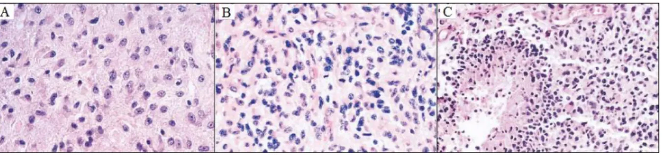
Analysis of the most malignant region of the tumours establishes grading, which is based on the degree of nuclear atypia, mitosis, microvascular proliferation and necrosis (Figure 1.6). Grade I applies to lesions with low proliferative potential and the possibility of cure following surgical resection alone. Neoplasms designated grade II are generally infiltrative in nature, and despite low-level proliferative activity, often recur. Some type II tumours tend to progress to higher grades of malignancy. The designation WHO grade III is generally reserved for lesions with histological evidence malignancy, including nuclear atypia and brisk mitotic activity. Lastly, the designation WHO grade IV is assigned to cytologically malignant, mitotically active, necrosis-prone neoplasms typically associated with rapid pre-postoperative disease evolution and a fatal outcome [39].

Figure 1.6 - Histologic criteria of the WHO for the classification of gliomas. (A) Fibrillary astrocytoma is

characterized by increased cellularity. (B) Anaplastic astrocytoma is characterized by nuclear atypia and mitoses. (C) Glioblastoma multiform is characterized by necrosis with cells arranged around the edge of the necrotic tissue (adapted from [40]).

1.4.1. Low-grade Gliomas

Low-grade gliomas correspond to WHO grades I and II. There are 3 subtypes of low-grade gliomas: pilocytic astrocytoma, astrocytoma and oligodendroglioma [10].

Astrocytomas are tumours found in young adulthood, with a peak incidence in the third or fourth decade of life. They arise from astrocytes, star-shaped glial cells in the brain and spinal cord that, among other functions, provide biochemical support of the endothelial cells that form the BBB. Typically, the first clinical manifestation is a seizure, which may be accompanied or followed by other neurological symptoms or signs. The diagnosis is usually established when neuroimaging is performed to evaluate the seizure. In patients presumed to have low-grade gliomas, MRI is supplemented by PET, since these tumours are characterized by glucose hypometabolism. PET images showing diffuse hypometabolism may support a decision to defer surgery or radiation therapy. If hypermetabolic areas are present,

11

indicating the presence of a high-grade tumour, biopsy or resection should target those areas in an effort to include the most malignant tissue in the tumour volume [39, 40].

Because most patients with astrocytoma are young and neurologically normal, treatment is particularly challenging. When the lesion is amenable to complete surgical excision, resection is performed. However, the majority of the low-grade tumours are not amenable to resection because they involve too large an area of the brain, or are too close to critical structures.

Most astrocytomas progress to high-grade malignant gliomas, which are often marked by hypermetabolic areas on PET scans. The median survival of patients with low-grade astrocytomas is 5 years, and most patients die from progression of their disease to a high-grade malignant glioma [40].

Oligodendrogliomas and oligoastrocytomas are tumours of oligodendrocytes or their precursors. Oligodendrocytes are a type of neuroglia which function is to provide support and insulation to axons in the central nervous system. The majority of oligodendrogliomas are low-grade and radiographically indistinguishable from astrocytomas, although oligodendrogliomas are more likely to be calcified. These oligodendroglial tumours are prone to spontaneous haemorrhage, as a result of their delicate vasculature. Most patients present a seizure, or progressive hemiparesis, or cognitive impairment.

The issues concerning diagnosis and treatment are identical to those for low-grade astrocytomas. Treatment is deferred until there is clinical or radiologic evidence of progression, unless patients have disabling symptoms or signs at presentation. However, once the decision to initiate treatment is made, the therapy differs from that for astrocytomas.

Eventually, most oligodendrogliomas, like astrocytomas, progress by becoming malignant. Patients with worsening clinical symptoms and the appearance of hypermetabolism on PET scans warrant re-evaluation.

1.4.2. High-grade Gliomas

High-grade gliomas are classified as malignant astrocytomas, anaplastic astrocytoma, and glioblastoma multiforme. These are also the most common glial tumours. Gliomas can occur anywhere in the brain, but usually affect the cerebral hemispheres. The male to female ratio among affected patients is about 3:2. The peak age at onset for anaplastic astrocytomas is in the fourth or fifth decade, whereas glioblastomas usually present in the sixth or seventh decade [40].

The glioblastoma multiform is the most malignant and most common glioma. There are two types of glioblastomas, and they arise through different molecular pathways. Primary glioblastomas arise alone and are associated with a high rate of overexpression or mutation of the epidermal growth factor receptor, p16 deletions, and mutations in the gene for phosphotase and tensin homologues. Secondary glioblastomas arise from a pre-existing low-grade tumours. In a secondary glioblastoma, a low-grade tumour may be immediately adjacent to a highly malignant disease. Error can occur when a small sample is taken for biopsy and the examined tissue does not reflect the biology of the entire tumour, particularly if features indicative of malignancy are missed. All gliomas, particularly the astrocytic neoplasms, are histologically, genetically, and thus therapeutically heterogeneous [40].

Primary glioblastomas tend to occur in older patients (mean age, 55 years), whereas secondary glioblastomas occur in younger adults (45 years old or less). The histologic features of the tumour and the age and performance status of the patient are major prognostic factors on outcome [10,40].

Malignant gliomas are surrounded by edema, and the mass effect can be severe enough to cause herniation. The tumour typically involves white matter and can spread across the corpus callosum and involve both hemispheres. These tumours are widely infiltrative. Tumour cells typically extend microscopically several centimeters away from the obvious area of disease and, in some cases, can extend throughout large portions of the brain. This condition is known as gliomatosis [10,40].

12

The treatments for anaplastic astrocytoma and glioblastoma multiform are identical. Resection is the initial intervention. Gross total excision is associated with longer survival, and improved neurologic function; therefore, every effort should be made to remove as much tumour as possible. Radiotherapy and additional chemotherapy are also prescribed. However, despite aggressive treatment, most patients die of the disease, with median survival of about 3 years for anaplastic astrocytoma, and one year for glioblastoma.

Oligodendrogliomas can also be classified as high-grade. These anaplastic oligodendrogliomas, like malignant astrocytic tumours, require immediate treatment after diagnosis. Extensive resection should be performed if feasible.

1.5. Imaging of Brain Tumours

As previously stated, the degree of malignancy plays a crucial role in assessing the prognosis of glioma patients and in planning appropriate individual management. Therefore, tissue diagnosis (biopsy) is the current diagnostic gold standard for determining tumour grade, which in turn forms the basis for subsequent treatment decisions. Generally a biopsy procedure is safe, but complications, such as bleeding or infection, may occur. In some cases, the amount of tissue obtained from a needle biopsy may not be sufficient or the procedure is unable to detect some lesions. The biopsy may then have to be repeated or surgical biopsy will be necessary. Hence, non-invasive alternatives for tumour diagnosis are sought after. The value of PET using radiolabeled amino acids or analogues for non-invasive tumour grading remains controversial [41]. The following section provides an overview of the studies performed to determine the diagnostic value of FET in brain tumours, including comparisons with other widely used tracers and imaging techniques.

1.5.1. Comparison between FET PET and FDG PET

The diagnostic value of PET using FDG and FET in patients with brain lesions suspicious of cerebral gliomas was studied [43]. Within a 2-year period, a group of 59 adult patients admitted with suspicion of a cerebral glioma or a recurrence of a previously operated glioma was studied with FET and FDG PET. The patients were examined on the same day prior to a neuronavigated biopsy or open surgery. Preoperative MRI, FET and FDG PET scans were co-registered and evaluated by ROIs using dedicated software. From the initial 59 patients, 52 were analysed. 43 patients had diffuse gliomas, of whom 33 had primary tumours and 10 recurrences. The extent of the tumour could be clearly delineated in each patient. In 33 of 43 patients a local maximum could be identified on FET scans for biopsy guidance. On the other hand, only 15 of the 43 patients had elevated FDG uptake. The definition of tumour extent remained impossible in every case due to high FDG uptake in the grey matter. Thus, FET proved to be clearly superior to FDG PET for biopsy guidance and treatment planning of cerebral gliomas, since FET identified a metabolic hot spot in the tumour area in 76% of the patients (33 out of 43), while FDG showed focally increased uptake in 28 gliomas only (out of 43).

Another study in patients with suspected or known brain tumours was performed by Lau et al. [44]. The aim of the study was also to establish the diagnostic value of FET PET when compared with FDG PET. Twenty-five FET PET and FDG PET scans were performed on 21 patients within 24 months. Final malignant pathology included 11 gliomas, 8 of which were low-grade, and three high-grade. FET PET was 100% accurate in the assessment of low-grade gliomas, while FDG PET has a sensitivity of only 13%. Also, FET PET had a 67% sensitivity for high-grade glioma against 33% sensitivity of FGD PET. The evaluated group of patients also comprised two lymphomas, one olfactory

13

ganglioneuroblastoma, and one anaplastic meningioma. FET PET was 100% accurate in the lymphoma group. Benign pathology included two encephalitis and one cortical dysplasia. Definitive pathology was not available for 3 patients. The accuracy of PET was determined by subsequent surgical histopathology in 12 patients and clinical/imaging course in nine patients. Median follow-up period was 20 months.

The predominant clinical indication for initial PET in this study was suspected recurrent tumour following previous treatment, representing a subgroup of 14 out of 21 patients. Of these, 7 patients had a history of glioma, 5 had cerebral lymphoma. In this category, FET PET had a sensitivity of 89%, specificity of 100% and accuracy of 93%. On the other hand, FDG PET had a sensitivity of 33%, specificity of 80% and accuracy of 50%. No lesion was correctly classified by FDG PET that had not also been correctly diagnosed by FET PET. These results show that FET is superior to FDG as a PET tracer in the assessment of suspicious brain lesions, especially in low-grade glioma.

In the light of studies regarding the diagnostic potential of FET in gliomas, Pauleit et al. [45] investigated the usage of FET PET in patients with squamous cell carcinoma (SCC) of the head and neck region by comparing that tracer with FDG PET and CT. Twenty-one patients with suspected head and neck tumours underwent FET PET, FDG PET and CT within one week before operation. After co-registration, the images were evaluated by 3 independent observers and a Receiver Operating Characteristic (ROC) analysis was performed, with the histopathological result used as a reference. The maximum SUVs were also determined. In 18 of 21 patients, histological examination revealed SCC, and in 2 of these patients, a second SCC tumour was found at a different anatomic site. In 3 of 21 patients, inflammatory tissue and no tumour were identified by histology. Eighteen of 20 SCC tumours were positive for FDG and FET uptake. One 3.0 cm tumour was detected neither with FDG PET nor with FET PET. In a different patient, histological examination showed a 0.7 cm tumour in a 4.3 cm inflammatory ulcer. The FDG PET scan overestimated the carcinoma as a 4 cm lesion with increased FDG uptake, while the scan obtained with FET missed this small carcinoma. All carcinomas with increased FET uptake exhibited concordant FDG accumulation, and no additional lesion could be identified with FET PET. Furthermore, the SUVs for SCC were higher in all cases with FDG than with FET. Overall, the sensitivity of FDG PET was 93%, specificity was 79% and accuracy was 83%. FET PET yielded a lower sensitivity of 75%, but a higher specificity (95%), and an accuracy of 90%.

According to these results, because uptake and sensitivity are lower for FET than for FDG, FET does not represent an ideal tracer for the evaluation of primary SCC of the head and neck region. However, the higher specificity makes FET PET an interesting additional tool in the follow-up of patients with SCC. Thus, FET may not replace FDG in the PET diagnostic of head and neck cancer, but may be a helpful additional tool in selected patients by allowing better differentiation of tumour tissue from inflammatory tissue [45].

1.5.2. Comparison between FET PET and MRI

In another study, the diagnostic accuracy of FET PET and MRI was compared in 45 patients, 36 of which with gliomas and neurological diagnosis of tumour recurrence, while the remaining 9 had undergone radioimmunotherapy [46]. FET PET and MRI studies were performed in all patients. Tumour recurrence was documented in 31 of 45 patients. FET PET and MRI revealed a correct diagnosis in 44 and 36 patients respectively, and the difference was statistically relevant (P<0.01). Specificity and sensitivity of FET PET were 92.9% and 100% respectively, against 50% and 93.5% of MRI. The results confirmed FET PET as a powerful tool to distinguish between benign side effects of therapy and tumour recurrence in patients with gliomas.

Prognostic factors in adult patients with untreated, nonenhancing, supratentorial low-grade glioma were studied by Floeth et al. [47], with special regard to FET PET and MRI. FET PET and MRI

14

analysis were performed on 33 patients with histologically confirmed low-grade glioma. None of the patients had radiation or chemotherapy. Clinical, histological, therapeutical, FET uptake and MRI morphologic parameters were analysed for their prognostic significance. Baseline FET uptake and a diffuse versus circumscribed tumour pattern on MRI were highly significant predictors of prognosis (P<0.01). By the combination of these prognostically significant variables, 3 major prognostic subgroups of low-grade glioma patients could be identified, and the statistical analysis proved that they had significant survival differences. The first of these subgroups was composed of patients with circumscribed low-grade glioma on MRI without FET uptake. Progression occurred in 18% of the cases, and there were no signs of malignant transformation and no death. The second subgroup was patients with circumscribed low-grade glioma with FET uptake. For this subgroup, progression occurred in 46% of the cases, malignant transformation to a high-grade glioma occurred in 15% of the cases, and death rate was of 8%. The last subgroup was patients with diffuse low-grade glioma with FET uptake. Progression occurred in all cases, malignant transformation in 78%, and death in 56%. Given these results, the authors concluded that baseline amino acid uptake on FET PET and a diffuse versus circumscribed tumour pattern on MRI are strong predictors for the outcome of patients with low-grade glioma.

As mentioned in previous sections, brain tumours are histologically heterogeneous. MRI-guided stereostatic biopsy does not always yield a valid diagnosis or tumour grading, because some regions of the nonenhancing tumours may be high-grade. Accurate grading and diagnosis are especially important for directing the therapeutic approach and providing the prognosis in patients with nonresectable tumours. The added value of FET in diagnostic accuracy of MRI for location and extent of cerebral gliomas was investigated in [48]. PET with FET and MRI were performed on 31 patients with suspected cerebral gliomas. PET and MRIs were co-registered and 52 neuronavigated tissue biopsies were taken from lesions with both abnormal MRI signal and increased FET uptake, as well as from areas with abnormal MR signal but normal FET uptake or vice versa. The diagnostic performance for the identification of cellular tumour tissue was analysed for either MRI alone or MRI combined with FET PET using alternative free response receiver operating characteristics curves (ROCs). FET findings were negative in 3 patients with an ischemic infarct and demyelating disease, and these 3 patients were excluded from the study. Tumour was diagnosed in 23 out of the 28 remaining patients, and reactive changes were found in the other 5. The diagnostic performance of MRI alone was compared with that of MRI combined with FET. MRI yielded a sensitivity of 96% for the detection of tumour tissue but a specificity of only 53%; FET PET alone yielded a sensitivity of 93% and a specificity of 81%. Finally, combined use of MRI and FET PET yielded a sensitivity of 93% and a specificity of 94%. Given these results, the authors of the study concluded that combined use of MRI and FET PET significantly improves the accuracy of the distinction of cellular glioma tissue from peritumoural brain tissue. Combined MRI ad FET diagnostics seems to be especially useful in brain lesions without BBB disruption.

The follow-up of glioblastoma patients after radiochemotherapy with conventional MRI can be difficult since reactive alterations to the BBB with contrast enhancement may mimic tumour progression. This phenomenon has been termed pseudo progression (PsP), and is a consequence of subacute treatment-related local tissue reaction, which comprises inflammation, edema, and increased permeability of the BBB [49]. PsP occurs with or without clinical deterioration, though interestingly it seems to be associated with a better outcome, and it is more common between patients that are more responsive to temozolomide treatment [50]. The reliable differentiation of early tumour progression (EP) from PsP is crucial since PsP spontaneously resolves without changing the standard treatment and a correct diagnosis may prevent unnecessary and potentially harmful change in treatment. On the other hand, the reliable detection of tumour progression at an early stage is essential for optimizing the treatment strategy in the individual patient.