M
ASTER
F
INANCE
M
ASTERS
F
INAL
W
ORK
D
ISSERTATION
T
ESTING THE RANDOM WALK HYPOTHESIS IN THE
U.S
TREASURY YIELD CURVE WITH VARIANCE RATIO
STATISTICS
J
OÃO
L
UÍS
D
A
S
ILVA
L
AINS
C
OMMITTEE
M
EMBERS
:
J
OÃOA
FONSOR
IBEIROF
ERREIRAB
ASTOSA
NÍBALJ
ORGE DAC
OSTAC
RISTOVÃOC
AIADOC
LARAP
ATRICIAC
OSTAR
APOSO2
Abstract
The random-walk hypothesis in the U.S. treasury yield curve was not previous studied and is surprising that researchers do not filled that void by testing it. However, the U.S treasury securities market is a benchmark, as the U.S treasury is considered to be risk-free. This benchmark is used to forecast economic development, to analyse securities in other markets, to price other fixed-income securities and to hedge positions taken in other markets. This study applies Chow Denning (1993) multiple variance test, Joint wright multiple version of Wright’s rank and sign tests, Choi (1999) Automatic Variance ratio Test and we also use the well-known Augmented Dickey-Fuller unit roots test to enable us to define the methodology to be used in the study. The database used permits the estimation of relative daily variation on U.S. treasury yield curve from January 1980 to December 2014. We hope that this analysis can provide useful information to traders and investors and will make a contribution in assisting to understand the pattern and behaviour of yields movement.
3
List of Abbreviations
ADF – Augmented Dickey-Fuller Test EMH – Efficient Market Hypothesis FED – Federal Reserve
PY – Par Yield
RWH - Random Walk Hypothesis U.S. – United States Of America VR – Variance Ratio Tests ZC – Zero-Coupon Yield
List of Tables
I. Descriptive Statistics for Relative Daily Variation of U.S. treasury yields II. Variance Ratio Tests on 1 Year Zero-Coupon Yields
III. Variance Ratio Tests on 5 Years Zero-Coupon Yields IV. Variance Ratio Tests on 10 Years Zero-Coupon Yields
V. Variance Ratio Tests on 20 Years Zero-Coupon Yields VI. Variance Ratio Tests on 1 Year Par Yields
VII. Variance Ratio Tests on 5 Years Par Yields VIII. Variance Ratio Tests on 10 Years Par Yields
IX. Variance Ratio Tests on 20 Years Par Yields
X. Augmented Dickey-Fuller Unit Root Test on Zero-Coupon and Par Yields
4
List of Figures
1 Selected Data of Observations for ZC yields (1980 to 2014) 2 Selected Data of Observations for PY yields (1980 to 2014)
3 Relative Daily Variation of U.S treasury yield curve (R Software Plot) 4 Augmented Dickey-Fuller Unit Root Test outcome
5 Chow and Denning (1993) Multiple Variance Ratio Test on ZC yields curve 6 Chow and Denning (1993) Multiple Variance Ratio Test on Par yields curve 7 The Automatic Variance ratio test of Choi (1999) on ZC yields curve 8 The Automatic Variance ratio test of Choi (1999) on Par yields curve
5
Acknowledgment
First of all I wish to thank my supervisor Professor João Bastos for his constant availability and support.
Special thanks to my family, friends and colleagues for all the support and encouragement that gave me and for have never let me give up.
6
Contents
1. INTRODUCTION 7
2. LITERATURE REVIEW 9
2.1. RANDOM WALK HYPOTHESIS 9
2.2. YIELD CURVE 10
3. METHODOLOGY 11
3.1. UNIT ROOT TEST 11
3.2. MULTIPLE VARIANCE TEST BY CHOW AND DENNING (1993) 12 3.3. NON-PARAMETRIC VARIANCE RATIO TESTS USING RANKS 13
AND SIGNS BY WRIGHT (2000)
3.4. AUTOMATIC VARIANCE RATIO BY CHOI (1999) 18
4. DATA 20
5. DESCRIPTIVE STATISTICS 23
6. EMPIRICAL RESULTS 24
6.1. OUTCOME OF THE TESTS 24
6.2. THE DECADE OF 1980 30
6.3. ECONOMIC EXPANSION AFTER 1990 31
6.4. QUANTITATIVE EASING (QE) 32
7. CONCLUSION 33
8. REFERENCES 34
7
1.
Introduction
The U.S. treasury market is one of the most liquid markets in the global financial system. According to the Securities Industry and Financial Markets Association (SIFMA) data, the outstanding U.S. treasury market debt in 1980 was 623.2 billion dollars, climbing up to 12504.8 billion dollars in 2014, on average 4009.5 billion dollar per year over the 34 years and there is also a huge evidence of a market grow after 2008 until 2014 where the average is 9604.4 billion dollars per year. The “primary dealers” are the so-called main players of the market that are allowed to trade directly with the Federal Reserve: Commercial banks, investment banks, large securities broker-dealers and central banks. This major participants purchase the majority of the treasury securities issued and distribute them in what is known by the “secondary market”. Treasurers and fund managers keenly follow the yield curve, as this helps them to manage or guard their exposures to other investments and protect themselves against unfavourable yield movements using risk management tools. The U.S. treasury yield curve is interesting not only to academics, but to these main players as well, since higher knowledge about the markets may lead them to better decision-making in terms of trade policy (strategies).
Information about the behaviours of The U.S. treasury yield curve, in terms of randomness, is really important to all players including academics (Belaire-Franch & Opong 2005) and for some years the random walk hypothesis discussion has been popular. There are some empirical studies concerning testing the RWH (Liu and He (1991), Huang (1995)) the increasing interest in the market efficiency attract academicians and practitioners. Academicians would like to better know the return patterns of financial assets. Practitioners attempt to identify the market inefficiency to develop trading strategies. Nowadays, the availability of new market data, the longer study period, and more methodologies satisfy academicians’ and practitioners’ interest.
8
Regarding methodology available to test the RWH, variance ratio tests are considered really powerful. Chow-Denning (1993) modify Lo-MacKinlay (1988) test to form a simple multiple variance ratio test, Joint wright multiple version of Wright’s (2000) rank and sign tests to address the potential limitations of Lo-McKinlay’s test and Choi (1999) Automatic Variance ratio Test that address for the better choice of the holding period of the test.
Clearly, the study seeks to investigate whether successive relative daily variations of the yields in the U.S. treasury market follow a random walk process and its relation with chronologic events in the U.S. economy. This study will make a contribution in assisting to understand the pattern and behaviour of yields movement as well as fill the lack of investigation with the RWH on the U.S. treasury yield curve.
9
2.
Literature review
2.1. Yield curve as a leading indicator
A yield curve represents the relationship between interest rates and the remaining time to maturity. Forecasting of the yield curve can provide significant information for monetary policy and the development of models for forecasting yield curves is of fundamental importance to banks, financial institutions and future economic activity. One reason for this, is the fact that some authors have been showing that the slope of the yield curve contains crucial information about the future path of macroeconomic variables in a number of countries.
For example, Fama (1990) and Mishkin (1990) show that spreads between long and short-term interest rates have information that permit predict future inflation in the U.S. Jorion and Mishkin (1991) show that term spreads also contain data about inflation in the U.S, Germany, Switzerland and the United Kingdom.
Bernanke (1990) and Estrella and Hardouvelis (1991) show that term spreads are useful for anticipate real economic growth in the U.S., Plosser and Rouwenhorst (1994) present evidence that term spreads contain information for predicting real economic growth in the U.S., Canada and Germany, but not in France and the United Kingdom. Furthermore, using data for the U.S., Germany and the United Kingdom, they demonstrate that foreign term spreads are useful for predicting future real economic growth in the domestic economy. Estrella and Mishkin (1995b) study if the term structure can predict recessions in France, Germany, Italy, the United Kingdom and the U.S., they discover that the term structure predicts recessions really accurately in the U.S. and Germany, United Kingdom and Italy. However, in France the term structure does not contain information useful for predicting recessions.
Haubrich and Dombrosky (1996) observe that the public anticipates that short-term interest rates will decline gradually in a recession until the economy’s performance improves.
10
These reductions in short-term interest rates may stem from countercyclical monetary policy designed to stimulate the economy, or they may simply reflect low real rates of return during the recession. In either case, the anticipated severity and duration of the recession will strongly influence the expected path of short-term interest rates, which will show.
These studies show the influence level of the yields curve as an indicator for prediction of crisis or economic expansion periods on the world’s economy. It illustrates the importance of our main focus on the RWH on the U.S. treasury yield because our results can provide additional or complementary information to all the literature existent on this field.
2.2. Random Walk Hypothesis
The RWH literature in financial time series has been highly studied during the 20th century. If the time series of an asset follows a random walk, then is very unlikely to predict the returns and investors are unable to make abnormal returns over time. Regarding to the efficient markets hypothesis (EMH), a market is efficient if stock prices reflect all available information, meaning that future prices cannot be predicted in advance (Fama, 1965). The random walk issue is strongly connected to the efficiency of the market and this subject is relevant for all market participants, as well as, researchers. Although there have been a lot of studies which test for the random walk hypothesis in assets price, most of them are focused on developed markets and emerging markets among all continents.
Some well-known and recognized studies on market efficiency are: Kendall (1953), he analysed prices of some assets, including stocks and commodities in Chicago’s market, concluding that the behaviour of the prices were completely random; Osborne (1964), Fama (1970), Trippi & Lee (1996), contributed to prove the existence of an unpredictability in the markets behaviour.
The Variance ratio tests approach of the random walk hypothesis were founded by Lo and MacKinlay (1988), and it is the most relevant study on the random walk hypothesis.
11
However, the test works on testing one variance ratio at a time for a single observation interval. Chow & Denning (1993) have suggested that a proper test of the random-walk hypothesis should be based on multiple comparison of a set of variance ratios in order to have a correct overall size of the test, which requires a joint hypothesis test of the original test. Over the years, other tests were developed to improve and remedy lacks of the previous models, for example the Whang & Kim (2003) subsampling test, Kim (2006) wild bootstrap test and Wright (2000) non-parametric ranks and signs tests. After all, the Lo and MacKinlay (1988) methodology remains one of the most powerful tests.
Choi (1999) tests the random walk hypothesis for the log-differenced monthly U.S. real exchange rates versus some major currencies, using the automatic variance ratio test and other test for serial correlation. The tests reject the null hypothesis at conventional significance for Japan, Switzerland and Great Britain.
Poterba and Summers (1988) and Lo and MacKinlay (1988) studied Western markets and apply multiple variance ratios to test the random walk in six equity markets using both monthly and daily data. There was no rejection of the null hypothesis of random walk in all six markets using monthly data. Analysing daily data, they rejected the RWH for France, Germany, UK and Spain but not for Greece and Portugal.
Worthington and Higgs (2004) run a research on twenty European country markets using well-known methodologies: serial correlation test, runs test, Augmented Dickey-Fuller test and a variance ratio test. They come with the result that just five countries out of twenty follow a random walk, particularly, Germany, Ireland, Portugal, Sweden and the United Kingdom, however France, Finland, the Netherlands, Norway and Spain meet only some of the requirements for a random walk.
Chen (2008) utilizes Lo-MacKinlay’s (1988) conventional variance ratio test, Chow-Denning’s (1993) simple multiple variance ratio test, and Wright’s (2000) non-parametric ranks- and signs-based variance ratio tests to test the random-walk hypothesis of the
12
Euro/Dollar exchange rate market from January 1999 to July 2008. They do not reject the random-walk hypothesis and conclude that the Euro/Dollar exchange-rate market is observed as weak-form efficient. Rashid (2006) achieved the conclusion that Pakistan there is evidence for the random-walk hypothesis in five pairs of weekly nominal exchange rates using Lo and MacKinlay’s (1988) variance ratio tests.
While the last methodological advances in testing the random walk were focused on stock prices, indexes and exchange rates, this paper attempts to bridge the lack of research on the treasury market by employing variance ratio tests to examine the RWH for the U.S. treasury yields curve. We contribute to the literature on the random walk hypothesis by reporting conclusions based on variance ratio tests. A further contribution is that, compared with previous market studies this sample is larger and more accurate due to the source Gürkaynak, Refet S., Brian Sack, and Jonathan H. Wright (2007) "The US Treasury yield curve: 1961 to the present”.
13
3.
Methodology
The study utilizes the variance ratio methodology developed by Chow and Denning (1993), Wright (2000)’s ranks and signs non-parametric VR tests and Automatic Variance Ratio Test by Choi (1999). We also make use of the well-known Augmented Dickey-Fuller unit root test to test the autocorrelations in the series and to define the methodology to be used in this paper, it is important to note the implication of the RWH. We want to test if the fluctuations on the U.S treasury yields are unpredictable, meaning that the successive values on our time series are not correlated and the time series does not follow a unit root.
3.1. Unit Root Test
We apply the well-known unit root test, namely the Augmented Dickey-Fuller (ADF) test. This test is used to examine unit root in a time series. The most common tests are the Augmented Dickey-Fuller (ADF) test, the Phillips-Perron (PP) test and Kwiatkowski, Phillips, Schmidt and Shin (KPSS) test. The null hypothesis is that the series have a unit root (the index series is non-stationary), while the latter tests if it represents a stationary process (no unit root). Another way to deal with stochastic trends (unit root) is by taking the first difference of the variable. If the series is non-stationary and the first difference of the series is stationary, the series contains a unit root or does not follow the random walk.
We run this test on the relative variation on U.S. treasury yield curve and expect the relative variation series to be integrated of order zero, I(0). The null hypothesis is that the series is non-stationary (unit root). We apply the following regression model of the ADF test:
Model: ∆yt = c0+ c1t + δyt−1+ β ∑i=1p ∆yt−1+ μt (1)
Model (trend and intercept) includes a constant term 𝑐0 and a trend term 𝑐1; p is the number
14
3.2. Multiple Variance Test by Chow and Denning (1993)
Chow and Denning (1993) point out that failing to control the test size for variance ratio estimates result in large Type I errors. To control the test size and reduce the Type I errors, Chow and Denning (1993) extends Lo-MacKinlay’s (1988) conventional variance ratio test methodology and form a simple multiple variance ratio test, which uses Lo-MacKinlay test statistics as the studentized maximum modulus (SMM) statistics.
Consider a set of variance ratio estimates, {VR (qi) | i = 1, 2, 3,…, L}, corresponding to a set of pre-defined number of lag {qi | i = 1, 2, 3,…, L}. Under the null hypothesis of random walk, we test a set of sub hypotheses, H0i: VR (qi) = 1 for i = 1, 2, 3,…, L. Since
any rejection of H0i will lead to the rejection of RWH, let the largest absolute value of the
test statistics be
CD1(q) = max1≤i≤L|CD(qi)| (2)
CD2(q) = max1≤i≤L|CD∗(qi)| (3)
Where CD(qi) and CD*(qi) are defined by:
The standard normal test statistic used to test the null hypothesis of random walk under the assumption of homoscedasticity is CD(q), calculated as:
CD(q) = (VR (q)−1)√θ(q) ~N(0,1) (4) Where
θ(q) =2(2q−1)(q−1)3q(nq) (5)
The standard normal test statistic used for heteroskedasticity-consistent is CD*(q), calculated as:
15 CD∗(q) = (VR (q)−1) √θ∗(q) ~N(0,1) (6) Where θ∗(q) = ∑ [2(q−j) q ] 2 q−1 j=1 δ̂(j) (7) And δ̂(j) =∑ (Xt−Xt−1−μ) nq t=j+1 2 (Xt−j−Xt−j−1−μ)2 [∑nqt=1(Xt−Xt−1−μ)2]2 (8)
The decision about whether to reject the null hypothesis can be based on the maximum absolute value of individual variance ratio test statistics. The test statistic follows the SMM distribution with L and T (the sample size) degrees of freedom, whose critical values are available in Stoline and Ury (1979). When the sample size T is large, the null hypothesis is rejected at α level of significance if 𝐶𝐷1(q) [or CD2(q)] is greater than the
[1 – (𝛼 ∗/2)] the percentile of the standard normal distribution where 𝛼 ∗= 1– (1 – 𝛼)1/ 𝐿. CD1(q) and CD2(q) have the same critical values. When T is large, the SMM critical values
at L = 4 and α equal to 10%, 5%, and 1% levels of significance are 2.23, 2.49, and 3.02, respectively.
3.3. Non-Parametric Variance Ratio Tests Using Ranks and Signs by
Wright (2000)
Wright (2000) indicates two potential advantages of ranks and signs based tests. First, it is very likely to calculate their exact distributions. The researchers do not need to concern about the size distortions due to no need to appeal to any asymptotic approximation. Second, tests based on ranks and signs may be more powerful than other tests if the data are highly non-normal. Wright (2000) proposes the alternative non-parametric variance ratio tests using ranks and signs of return and demonstrates that they may have better power properties than
16 other variance ratio tests.
Rank-Based Variance Ratio Tests
Suppose that 𝑌𝑡 is a time series of asset returns with a sample size of T.
𝑌𝑡 = 𝑋𝑡− 𝑋𝑡−1
Let 𝑟(𝑌𝑡) be the rank of 𝑌𝑡 among 𝑇1, 𝑇2… 𝑇𝑟, then 𝑟(𝑌𝑡) is the number from 1 to
T and given by:
r1t =
(r(Yt)−T+12 )
√(T−1)(T+1)12 (9)
r2t = ϕ−1(r(Yt)
T+1) (10)
Where 𝛷 is the standard normal cumulative distribution function and 𝛷 −1 is the inverse of the standard normal cumulative distribution function).
The series 𝑟1𝑡 is a simple linear transformation of the ranks, standardized to have
sample mean 0 and sample variance 1. The series 𝑟2𝑡, known as the inverse normal or van
der Waerden scores, has sample mean 0 and sample variance approximately equal to 1. Wright substitutes 𝑟1𝑡 and 𝑟2𝑡 in place of the return 𝑌𝑡= 𝑋𝑡− 𝑋𝑡−1 in the definition of
Lo-MacKinlay’s variance ratio test statistic.. The rank-based variance ratio test statistics R1 and R2 are defined as
R1 = ( 1 TK∑Tt=k(r1t+r1t−1…+r1t−k+1)2 1 T∑Tt=1r1t2 − 1) × (2(2k−1)(k−1)3kT )−1/2 (11) R2 = ( 1 TK∑Tt=k(r2t+r2t−1…+r2t−k+1)2 1 T∑Tt=1r2t2 − 1) × (2(2k−1)(k−1)3kT )−1/2 (12)
17 Note that 1T∑T r1t2 = 1
t=1 so that this term may be omitted from the definition of R1 in
equation (10), whereas 1 T∑ r1t 2 ≈ 1 T t=1 (13)
Sign-Based Variance Ratio Tests
For any series𝑌𝑡, let 𝑢(𝑌𝑡, 𝑞) = 1(𝑌𝑡> 𝑞) = 0.5. So, 𝑢(𝑌𝑡, 0) is 12. If 𝑌𝑡 is positive
and −12 otherwise. Let 𝑆𝑡 = 2𝑢(𝑌𝑡, 0) = 2𝑢(𝜀𝑡, 0) . Clearly, st is an independently and
identically distributed (iid) series with mean 0 and variance 1. Each 𝑆𝑡 is equal to 1 with
probability 12 and is equal to −1 otherwise. The signed-based variance ratio test statistic S1
is defined as S1 = ( 1 TK∑Tt=k(St+St−1…+St−k+1)2 1 T∑Tt=1St2 − 1) × (2(2k−1)(k−1)3kT )−1/2 (14)
Wright (2000) points out that S2 test is expected to have lower power. S2 is not
computed in this study.
Belaire-Franch and Contreras (2004) emphasize that it is possible to extend the idea of Chow and Denning (1993) to the tests proposed by Wright (2000). Thus, the joint tests of rank and sign is defined as follow:
JR1 = max
1≤i≤m|R1| (15)
JR2 = max1≤i≤m|R2| (16)
JS1 = max1≤i≤m|S1| (17)
This test follows a Studentized Maximus Modulus (SMM) distribution, with m and T degrees of freedom.
18
3.4. Automatic Variance Ratio Test by Choi (1999)
When implementing the VR tests, the choice of holding period k is important. However, this choice is usually rather arbitrary and ad hoc. To overcome this issue, Choi (1999) proposed a data-dependent procedure to determinate the optimal value of k. Choi (1999) suggested a VR test based in frequency domain since Cochrane (1988) showed that the estimator of V(k) which uses the usual consistent estimators of variance is asymptotically equivalent to 2π the normalized spectral density estimator at the zero frequency which uses the Bartlett kernel. However, Choi (1999) employed rather the Quadratic Spectral [QS] kernel because this kernel is optimal in estimating the spectral density at the zero frequency (Andrews, 1991). The VR estimator is defined as
VR̂ (l) = 1 + 2 ∑T−1k(
i=1 i l⁄ )ρ̂(i) (18)
ρ̂(i) = ∑T−1t=1 ∆rt∆rt+i/∑Tt=1∆rt2 (19)
where ρˆ(i) is the autocorrelation function, and h(x) is the QS window defined as
h(x) =12π252x2[sin (6πx 56πx 5⁄⁄ − cos (6πx 5⁄ )] (20) The standardized statistic is
VRf=(2)1 2VR(k)−1⁄ (T k⁄ )−1 2⁄ (21) Under the null hypothesis the test statistic VR follows the standard normal distribution asymptotically. Note that it is assumed that T → ∞, k → ∞ and T/k → ∞. Various methods for optimally selecting the truncation point for the spectral density at the zero frequency are available (Andrews, 1991; Andrews and Monahan, 1992; Newey and West, 1994; among others). Choi (1999) employed the Andrews’s (1991) methods to select the truncation point optimally and compute the VR test. Note that the small sample properties of this automatic VR test under heteroskedasticity are unknown and have not investigated properly.
19
4.
Data
The study utilizes the U.S. Treasury Yield Curve data from 1 January 1980 to 31 December 2014 primarily sourced from Gürkaynak, Refet S., Brian Sack, and Jonathan H. Wright (2007) "The US Treasury yield curve: 1961 to the present”. The Division of Research Statistics and Monetary affairs of the U.S. Federal Reserve Board data was published to stimulate discussion and provide benchmark yield curve that can be useful to applied economists. We extract the Zero-Coupon Yield and Par Yield curve (Figure 1 and 2, respectively) in order to calculate the relative daily variation for 1, 5, 10, 20 years maturities but the original data series includes a larger sampling of maturities (from 1-Year to 30-Years).
This period was chosen because it corresponds to the start of technological markets boom and to the period when most of the treasury yield maturities in analysis were available in the market, meaning that the 20-year maturity bonds just started in 1981. We apply the empirical tests in periods of 1 year during the whole study time using daily data. The yearly windows allow us to conclude accurately and with higher precision the impacts of the economy events on the relative variations of the yield curve.
20
Figure 1 – Selected Data of Observations for ZC yields (1980 to 2014)
Figure 2– Selected Data of Observations for PY yields (1980 to 2014) 0 2 4 6 8 10 12 14 16 18 Yie lds
Zero-Coupon Yields Curve
5 Year Zero-Coupon 2 Years Zero-Coupon 10 Years Zero-Coupon 20 Years Zero-Coupon
0 2 4 6 8 10 12 14 16 18 20 Yie lds
Par Yields Curve
21
On the figure 3, the relative daily variation of the yield curve is calculated in the usual format by taking the first differences of the natural logarithm of the yield as follows:
𝑌𝑡 = (𝑙𝑜𝑔𝑃𝑡− 𝑙𝑜𝑔𝑃𝑡−1) ∗ 100 (22) Where 𝑌𝑡 is the relative daily variation, 𝑙𝑜𝑔𝑃𝑡 is the natural logarithm of the present
day’s yield, and 𝑙𝑜𝑔𝑃𝑡−1 is the natural logarithm of the previous day’s yield.
22
5.
Descriptive Statistics
Table I gives the arithmetic mean, standard deviation, kurtosis and skewness of the Relative Daily Variation of the U.S treasury yields curve in study (figure 3). Observing the Zero-Coupon yields, the lowest means are in the 10 and 20 years yields while the highest mean is in the 1 year yields. The lowest minimum and highest maximum relative daily variation are in the 1 year yields: -0.4043 and 0.4012, respectively. The standard deviations of relative daily variation range from 0.01088 (20 years yields) to 0.033274 (1 year yields). The relative variations are positively skewed in almost all maturities, which means that large positive relative daily variations tend to be larger than the higher negative relative daily variation. Regarding the Par yields, the lowest means are in the 5, 10 and 20 years yields while the highest mean are the 1 year yields. The lowest minimum and highest maximum relative daily variation are in the 1 year yields: -0.4048 and 0.2709, respectively. The standard deviations of relative daily variation range from 0.0107 (20 years yields) to 0.0331 (1 year yields). The relative variations are positively skewed in 5 and 10 years maturities, however, negatively skewed in 1 and 20 years maturities. Note that on all the yields observed the level of kurtosis is high in the whole maturities, but with a tendency to decrease as the maturity years get longer. The Jarque-Bera statistic rejects the hypothesis of a normal distribution of returns in all maturities at a significance level of 1%.
Table I – Descriptive Statistics for Relative Daily Variation of U.S treasury yield curve
Yields Period No. of Obs. Mean Median Maximum Minimum Deviation Std. Skewness Kurtosis JB
ZC 1Y 1980 - 2014 8730 0.00042 0.00009 0.40124 -0.40437 0.033274 0.103 20.152 107021*** ZC 5Y 1980 - 2014 8730 0.00020 0.00027 0.24569 -0.14775 0.019824 0.044 13.995 43970*** ZC 10Y 1980 - 2014 8730 0.00017 0.00036 0.15521 -0.08559 0.013583 0.007 10.048 18066*** ZC 20Y 1981 - 2014 8355 0.00019 0.00037 0.07925 -0.07344 0.010882 -0.054 7.607 7392*** PY 1Y 1980 - 2014 8730 0.00042 0.00009 0.27094 -0.40485 0.033194 -0.034 18.502 87403*** PY 5Y 1980 - 2014 8730 0.00021 0.00026 0.24418 -0.14669 0.019816 0.045 13.830 42660*** PY 10Y 1980 - 2014 8730 0.00018 0.00030 0.15443 -0.08327 0.013566 0.009 9.729 16470*** PY 20Y 1981 - 2014 8355 0.00020 0.00036 0.07661 -0.07028 0.010733 -0.042 7.230 6229***
23
6.
Empirical Results
6.1. Outcomes of the tests
Unit Roots Test
Augmented Dickey-Fuller statistics test the null hypothesis of a unit root in the daily relative variation on the U.S. Treasury yield curve. Failure to reject the null hypothesis means that the random walk hypothesis is not rejected. We present the results of the Augmented Dickey Fuller test in the Figure 4 and the Table X of the appendix, the table shows the results for the relative daily variation on the Zero-Coupon and Par Yields defined as (22) refers.
The lag length of the ADF test is chosen based on the Akaike Information Criterion and the Schwarz Information Criterion method of setting the maximum number of lags at 6 for all years, except for 1981, 20 year maturity, due to less number of observations studied (Table X) . As we can see on the figure 4, the null hypothesis of unit root is strongly rejected as the t-statistic value of the ADF are lower than their critical values at 1% significance level which means that the relative daily variations tested for both Zero-Coupon and Par yields do not follow a random walk.
Figure 4 – Augmented Dickey-Fuller Unit Root Test outcome
-9.00 -8.00 -7.00 -6.00 -5.00 -4.00 -3.00 -2.00 -1.00 0.00 1980 1982 1984 1986 1988 1990 1992 1994 1996 1998 2000 2002 2004 2006 2008 2010 2012 2014
ADF - Unit Root Test
ZC1Y ZC5Y ZC10Y ZC20Y PY1Y PY5Y PY10Y PY20Y Rej90% Rej95% Rej99%
24
Multiple Variance Ratio Test by Chow and Denning (1993)
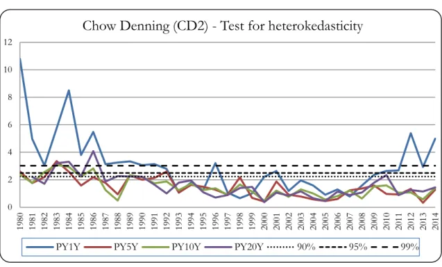
Chow and Denning (1993) through Lo and MacKinlay (1988) under heteroskedasticity show that the variance ratio test is more powerful than the Dickey-Fuller unit root test, and Ayadi and Pyun (1994) also argue that the variance ratio has more appealing features than other procedures. The figure 5 presents results of this variance ratio test for the Zero-Coupons yields curve and the figure 6 presents the results for the Par-Yield curve in analysis. We only present the CD2, test for uncorrelated series with possible heteroscedasticity, because normally this financial assets present conditional heteroskedasticity of yields. In order to get accurate results are used the selected lags: 2, 5, 10, and 20.
Figure 5 – Chow and Denning Multiple Variance Ratio Test on ZC yields curve
As we can observe on the figure 5, the hypothesis of a random walk is not rejected at 1% significance level for the whole period analysed (1980 to 2014) on the higher maturities: 5, 10, 20 Years, except the result in 1986 where the 20 Zero-Coupon yields get into the rejection zone at 1% significance level (Black Monday). For the lowest maturity, 1 Year Zero-Coupon yield, we can extract that only from 1992 to 2011 it fails to reject the Random Walk Hypothesis (economic expansion period). However, we can notice the impact of the “great moderation” before the 90’s, of the Taiwan crisis and the presidential elections in 1996 and
0 2 4 6 8 10 12 19 80 19 81 19 82 19 83 19 84 19 85 19 86 19 87 19 88 19 89 19 90 19 91 19 92 19 93 19 94 19 95 19 96 19 97 19 98 19 99 20 00 20 01 20 02 20 03 20 04 20 05 20 06 20 07 20 08 20 09 20 10 20 11 20 12 20 13 20 14
Chow Denning (CD2) - Test for heterokedasticity
ZC1Y ZC5Y ZC10Y ZC20Y
25
the QE effects after 2012, where the RWH is rejected at 1 % significance level.
Figure 6 – Chow and Denning Multiple Variance Ratio Test on Par Yields curve
On the figure 6, the hypothesis of a random walk is not rejected at 1% significance for the late 80’s period on the higher maturities: 5, 10 and 20 years, except in 1983, 1984 and 1986 where the results get heavily into the rejection zone at 1% significance level, meaning the impact of the Black Monday on the 20 Years Par Yields (also affecting the 5 and 10 years Par Yields in a lower scale). For the lowest maturity, 1 Year Par Yield, we can extract that only from 1992 to 2011 it fails to reject the Random Walk Hypothesis (economic expansion period). However, we can also observe the impact of the same events as on the Zero-Coupon Yield Curve.
The results obtained in both Yields Curve lead us to believe that before the 90’s and after the sub-prime crisis in 2008 the U.S. Treasury market was not weak form efficient, meaning that some events, that we will analyse later in this study, played a key role, having a big impact on the U.S. treasury yield curve behaviour.
0 2 4 6 8 10 12 19 80 19 81 19 82 19 83 19 84 19 85 19 86 19 87 19 88 19 89 19 90 19 91 19 92 19 93 19 94 19 95 19 96 19 97 19 98 19 99 20 00 20 01 20 02 20 03 20 04 20 05 20 06 20 07 20 08 20 09 20 10 20 11 20 12 20 13 20 14
Chow Denning (CD2) - Test for heterokedasticity
26
Non-Parametric VR Tests Using Ranks and Signs by Wright (2000)
In order complete some ambiguities in the results of the Lo and MacKinlay (1988) variance-ratios test regarding the relative daily variation behaviour in particular, we applied Wright’s (2000) version based on ranks and signs to further examine the Random Walk Hypothesis. The test takes the maximum value of the Wright’s rank or sign tests, in the same manner as Chow-Denning test through Lo and MacKinlay (1988). The tables II, III, IV and V present results for the Zero-Coupon yields and the tables VI, VII, VIII and IX present the results for the Par Yields in analysis (on the Appendix). We present the results of Wright’s test for the entire sample in a yearly basis. R1 and R2 report results of the rank based test whereas S1 presents the results of the sign based alternative. In order to get accurate results are used the selected lags: 2, 5, 10 and 20.
The R1, R2 and S1 fail to reject the null hypothesis of Random Walk at 1% significance level for the whole period analysed (1980 to 2014) on the higher maturities: 5, 10 and 20 Years, except the result in 1986 where the 10 and 20 Years Zero-Coupon yields get into the rejection zone at 1% significance level (Black Monday). For the lowest maturity, 1 year Zero-Coupon yield, we can extract that in R1 and S1 only from 1993 to 2011 fails to reject the null hypothesis and in R2 the random walk hypothesis is clearly not rejected from 1993 to 2010. However, we can highlight two important events contributing for the treasury market become not weak efficient in this years: the Taiwan Crisis and Presidential Elections in 1996 and the terrorist attacks of 2001.
On the Par Yields, the R1, R2 and S1 fail to reject the RWH at 1% significance level for the whole period analysed (1980 to 2014) on the higher maturities: 5,10,20 Years, except in 1983, 1984 and 1986 (Black Monday) where the results get into the rejected zone at 5% and 1% significance level. For the lowest maturity, we can extract that R1, R2 and S1 only from 1993 to 2010 it fails to reject the Random Walk Hypothesis (Economic expansion period).
27
Furthermore, the power of a test statistic of both ranks and signs increases with the lag, evidence that is also in line with Wright (2000). In addition, almost all rejections are in the upper tail of the null distribution, indicating that the resulting variance ratios are statistically greater than one at all lags for all the analysed series. The critical values for the Wright test used are 1.96, 2.23 and 2.76. They differ by the sample size n and have been generated through R Software, where we assume the n equal to the average number of observations each year, 250 observations, and we have used 10000 replications which is recommended by the author for better and accurate results.
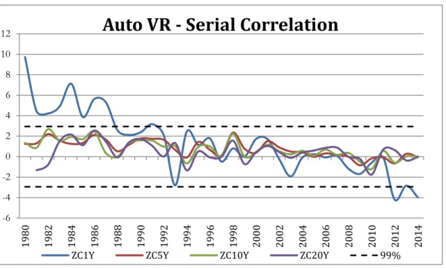
Automatic variance ratio test under conditional heteroskedasticity of Choi
(1999)
The Automatic Variance ratio test of Choi (1999) works under the null hypothesis of no serial correlation, which can help to interpret how well the past relative daily variation of a U.S treasury market predicts it future performance, the asymptotic distribution of the statistic has been found to be a two-sided test, the critical values are taken from both tails of the standard normal distribution. The tables II, III, IV and V presents results of this variance ratio test for the Zero-Coupons yields and the table VI, VII , VIII and IX presents the results for the Par-Yields in analysis
We find from the figure 7 and 8 as on the respective tables on the appendix that the null hypothesis of no serial correlation is not rejected for whole period on the 5,10,20 years yields. For the lowest maturity in study, 1 year yields, we observe the failure to reject the no serial correlation from 1992 to 2011. We may thus conclude on the basis of the findings of this test that from 1980 to 2014 the performance of the market on 5,10,20 years yields is weak form efficient as well as for the lowest maturity from 1992 to 2011, where we can find a period of economic and financial stability on the U.S economy.
28
Figure 7 – The Automatic Variance ratio test of Choi (1999) on ZC yields curve
Figure 8 – The Automatic Variance ratio test of Choi (1999) on Par Yields curve -6 -4 -2 0 2 4 6 8 10 12 1980 1982 1984 1986 1988 1990 1992 1994 1996 1998 2000 2002 2004 2006 2008 2010 2012 2014
Auto VR - Serial Correlation
ZC1Y ZC5Y ZC10Y ZC20Y 99%
-6 -4 -2 0 2 4 6 8 10 12 1980 1982 1984 1986 1988 1990 1992 1994 1996 1998 2000 2002 2004 2006 2008 2010 2012 2014
Auto VR - Serial Correlation
29
6.2. The decade of 1980 – “Great Moderation”
After proceed with the ADF Test and the variance ratio tests, we find that the U.S. market has implemented a series of innovations in the 1960’s and 1970’s, the automation and modernization of trading technology permitting foreign brokers/dealers on the floor; abolishment of fixed commissions; new regulations on corporate disclosure and auditing; extended trading hours and establishment of New York futures market, there is not weak form efficiency in the market that we can observe on the 1 Year maturity over the 80’s. This is also consistent with the findings of Gu and Finnerty (2002), but in contrast with Ito and Sugiyama (2009).
We can also identify on the figure 5 a reaction of the markets, on the longer maturities, in 1986 due to a stock markets crash. The Black Monday resulted from a shift on the growing recovery on the United States economy, which slowed the growing expansion in the late 1986. The world markets crash took place in 19th October 1987, after Hong Kong and West Europe hatted the U.S Market with significant declines in a very short period of time. During this period the U.S. Federal Reserve response set a precedent for the central banks use of liquidity to stem financial crisis as stretched by Cecchetti and Piti Disyatat (2010).
The “Great Moderation” is also an explanation for the non-random walk and not weak form efficiency of the market on the lower maturity yields. According to U.S. Federal Reserve Chairman Ben Bernanke the standard deviation of quarterly real GDP declined by half, and the standard deviation of inflation declined by two-thirds (see, for example, McConnell and Perez-Quiros, 2000; and Stock and Watson, 2002). With a more stable economy and accurate expectation, it was likely that the stock market become weak efficient and random, meaning it was not reflecting past events in future performance.
30
6.3. Economic expansion after 1990
The late years of the 80’s after the crash experienced much less occurrence of fundamental economic and political crises as well as the 10 years of economic expansion of the 1990s corroborating with the studies of R.thaler (1985), RJ Gilson RH Kraakman (1984), MC Jensen (1978), EF Fama (1998) to arrive at the conclusion that the U.S. Market was weak form efficient during this period. This form of efficiency has major implications for investors and market regulators. For investors, there is evidence that their return on investment will be guaranteed, as their capital allocation will be directed towards productive investment opportunities, ceteris paribus. Regulators on the other hand would find it necessary to reduce market interventions. This is consistent with the results obtained on the variance ratio tests, which indicates a period of random walk in all yield maturities studied.
The Chow And Denning (1993) and Wright (2000) tests results suggest that during this expansion period there were some events that influence the lower maturity yields random walk outcome. The Taiwan crisis and uncertainty of presidential election on U.S. increase the predictability of the market in 1996and in 2001 the effectiveness of the U.S. Federal Reserve as a central bank was put to the test on 11st of September 2001 due to the terrorist attacks on New York, Washington and Pennsylvania affecting U.S. financial markets. In the days after, the U.S. Federal Reserve lowered interest rates and loaned more than $45 billion to financial institutions in order to provide stability to the U.S. economy.
Due to the importance of the big financial crisis in 2007 and 2008 we analyse it influence in our outcomes. This impact is not significant in our analysis because the variance ratio test just reflect a light shift on the results tendency around 2007 and 2008 for the lowest maturity in study.However, the after sub-prime crisis the FED implemented new strategies to stimulate the economy, which we will develop in the next point.
31
6.4. Quantitative Easing (QE)
After the global financial crisis of 2007 and 2008, the United States of America, the United Kingdom, and the Eurozone used Quantitative Easing because their risk-free short-term nominal interest rates were close to zero. To control the situation and stimulate the economy, the U.S. central bank starts purchasing financial assets and monetary instruments from banks and financial institutes to lower long-term interest rates, which our VR tests strongly reflect. The implementation of the Quantitative Easing, known as QE, had three stages: QE1 took place in November 2008 until June 2010, where the Federal Reserve could inject 2.1 trillion into the United States economy; QE2 came in November 2010 because the economy was not growing as fast expected after QE1 and the plan was similarly spread over the next 8 months ending around June 2011; QE3 was implemented in September 2012, this QE was different from its predecessors because the plan was based on a monthly approach for purchases instead spend the whole budget for a period of time.
A significant event between QE2 and QE3 took place in September 2011, the Federal Reserve decided to introduce “Operation Twist. It was a quantitative easing in which the Federal Reserve sell its short-term Treasury Bills and use the funds to buy long-term Treasury Notes instead of buying short-term Treasury Bills again. This is consistent with the results of our variance ratio tests, where we reject the RWH and the markets are not weak efficient on lowest maturity in study from 2011 to 2012.
In June 2013, the Federal Reserve intend on taper the efforts to increase stability in the economy and was revealed that QE3 would be brought to a complete halt by the middle of 2014. However, our test outcomes indicate that the effects of the Quantitative Easing would be still present until the end of the year of 2014, meaning that we reject the null hypothesis for random walk with Chow Denning and Auto VR tests.
32
7.
Conclusions
In this research, the observation of the random walk hypothesis and the efficiency form present in the U.S. treasury yields curve, on a daily basis, are the main analysis focuses. The Augmented Dickey-Fuller test is used to check the existence of a unit root as a necessary condition for random walk is rejected over all the yield maturities tested. The VR tests permit identify clearly the biggest events in the U.S. economy chronology in the end of the 20th and
beginning of the 21st century, including recessions and economic expansion periods.
The Automatic Variance ratio test of Choi (1999) indicate the existence of no serial correlation on the longer yield maturities, meaning that we can’t use past to predict future outcomes on the U.S. treasury yield curve, and also confirm the sensibility of the 1 year maturity yields to events outside of economic expansion periods. The Chow Denning multiple VR test(1993) and Wright non-parametric VR test(2000) fail to reject the random walk hypothesis over all Zero-Coupon and Par Yield maturities during almost the whole period of study, except the lowest maturity that only fails to reject the RWH at the turn of the century. Therefore, we can conclude that as the lower are the yields maturity as the higher are its sensibility to economic events like recessions, terrorist attacks or new Federal Reserve monetary policies, meaning that market becomes not weak efficient. However, the random walk of U.S. treasury yields curve is directly affected by several events between 1980 and 2014 even in the highest maturities in analysis, which leads us to believe that there is still a big investigation margin on this field.
More than understand the random walk of the U.S. treasury yields curve or understand the impact of some chronologic events on the yield curve, would be also relevant to develop economic theories or monetary policies that will permit optimize anticipation and control of the yields curve outcome during several periods of time. To this become a reality, will be needed to apply VR tests to other benchmarks over all continents, other periodicities like weekly or monthly analysis and also other moving windows in different periods of the
33
world’s economy history. These are some examples of possible future researches that can be developed in this subject.
34
8.
References
Amélie Charles, Olivier Darné (2009). Variance ratio tests of random walk: An overview. Journal of Economic Surveys, Wiley-Blackwell, 23(3), 503-527.
Belaire-Franch, J. and Opong, K.K. (2005). Some evidence of random walk behaviour of
Euro exchange rates using ranks and signs. Journal of Banking and Finance, 29: 1631–1643.
Bernanke, B.S. (1990). On the predictive power of interest rates and interest rate spreads. New England Economic Review (Federal Reserve Bank of Boston), November/December, 51-68.
Cecchetti, Stephen G., and Piti Disyatat (2010). Central Bank Tools and Liquidity
Shortages. Federal Reserve Bank of New York Economic Policy Review 16, no. 1: 36-7
Choi, I. (1999). Testing the random walk hypothesis for real exchange rates. Journal of Applied Econometrics 14, 293–308.
Chow, K. V. and K. C. Denning (1993). A Simple Multiple Variance Ratio Test, Journal of Econometrics 58, 385-401.
D. Mbululu, C.J. Auret and L. Chiliba (2013), Do exchange rates follow random walks? A
variance ratio test of the Zambian foreign exchange market.
Eric Dongmo Guefack and Romuald N. Kenmoe S. (2013), Equity Stock Markets in
Africa: Empirical Evidence from the Random Walk Hypothesis.
Estrella, A. and G.A. Hardouvelis (1991). The term structure as a predictor of real economic
activity. Journal of Finance, 46(2), June, 555-76.
Estrella, A. and F. Mishkin (1995b). The term structure of interest rates and its role in
monetary policy for the European Central Bank. NBER working paper, 5279, September.
Fama, E.F. (1990). Term-structure forecasts of interest rates, inflation and real returns. Journal of Monetary Economics, 25(1), January, 59-76.
Gürkaynak, Refet S., Brian Sack, and Jonathan H. Wright (2007). The US Treasury
35
Gu, A. Y. Finnerty, J. (2002). The evolution of market efficiency: 103 years daily data of
Dow. Review of Quantitative Finance and Accounting, 18, 219-237.
Haubrich, J. G. and A. M. Dombrosky (1996). Predicting real growth using the yield curve. Federal Reserve Bank of Cleveland Economic Review, vol. 32(1), 26-35.
Ito, M. and Sugiyama, S. (2009). Measuring the degree of time varying market inefficiency. Economics Letters 103: 62-64.
Jeng-Hong Chen (2008). Variance Ratio Tests Of Random Walk Hypothesis Of The Euro
Exchange Rate. Albany State University, USA.
Jorion, P. and F. Mishkin (1991). A multicountry comparison of term-structure forecasts at
long horizons. Journal of Financial Economics, 29(1), March, 59-80.
Liu, C.Y. and He, J. (1991). A variance ratio test of Random Walks in foreign exchange
rates, Journal of Finance, 46(2): 773–785.
Lo, A. W. and A. C. MacKinlay (1988). Stock Market Prices Do Not Follow Random
Walks: Evidence from a Simple Specification Test. The Review of Financial Study 1, 41-66.
Kendall, M. (1953). The Analysis of Economic Time Series - Part 1: Prices. Journal of the Royal Statistical Society, 96, 11-25.
Kim, J.H. (2006). Wild bootstrapping variance ratio tests. Economics Letters, 92: 38–43. Maria Rosa Borges (2007). Random walk tests for the Lisbon stock market. Department of Economics, Technical University of Lisbon, Instituto Superior de Economia e Gestão.
Mishkin, F. (1990). The information in the longer maturity term structure about future
inflation. Quarterly Journal of Economics, 105 (3), August, 815-28.
Nityananda Sarkar (2001). Testing Market Efficiency in the framework of model
specification: an empirical investigation with Indian data. Indian Statistical Institute.
Plosser, C. I. and K. G. Rouwenhorst (1994). International term structures and real
36
Poterba, J. M. and Summers, L. H. (1988). Mean reversion in stock prices: Evidence and
implications, Journal of Financial Economics 22, 27–59.
Tomas K. Molenaars1 , Nick H. Reinerink1 , Marcus A. Hemminga (2013).
Forecasting the yield curve - Forecast performance of the dynamic Nelson-Siegel model from 1971 to 2008.
Trippi, R.R. and Lee, J.K. (1996). Artificial Intelligence in Finance and Investing:
State-of-the art Technologies for Securities Selection and Portfolio Management (Revised edition). BurrRidge, IL:
Irwin Professional Publishing.
Whang, Y.J. and Kim, J. (2003). A multiple variance ratio test using subsampling, Economics Letters, 79: 225–230.
Worthington A.C. and Higgs H. (2004). Random Walks and Market Efficiency in
European Equity Markets. Global Journal of Finance and Economics, 1(1), 59-78.
Wright, J. H., (2000). Alternative Variance-Ratio Tests Using Ranks and Signs. Journal of Business and Economic Statistics 18, 1-9.
37
9.
Appendix
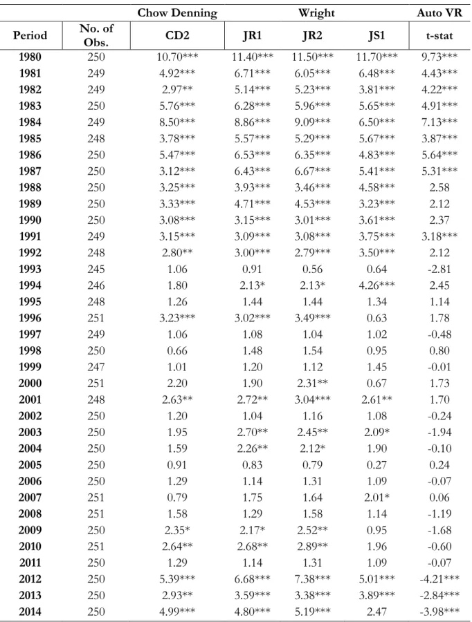
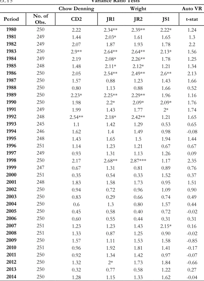
Table II - Variance Ratio Tests on 1 Year Zero-Coupon Yields
ZCY1 Variance Ratio Tests
Chow Denning Wright Auto VR
Period No. of Obs. CD2 JR1 JR2 JS1 t-stat
1980 250 10.70*** 11.40*** 11.50*** 11.70*** 9.73*** 1981 249 4.92*** 6.71*** 6.05*** 6.48*** 4.43*** 1982 249 2.97** 5.14*** 5.23*** 3.81*** 4.22*** 1983 250 5.76*** 6.28*** 5.96*** 5.65*** 4.91*** 1984 249 8.50*** 8.86*** 9.09*** 6.50*** 7.13*** 1985 248 3.78*** 5.57*** 5.29*** 5.67*** 3.87*** 1986 250 5.47*** 6.53*** 6.35*** 4.83*** 5.64*** 1987 250 3.12*** 6.43*** 6.67*** 5.41*** 5.31*** 1988 250 3.25*** 3.93*** 3.46*** 4.58*** 2.58 1989 250 3.33*** 4.71*** 4.53*** 3.23*** 2.12 1990 250 3.08*** 3.15*** 3.01*** 3.61*** 2.37 1991 249 3.15*** 3.09*** 3.08*** 3.75*** 3.18*** 1992 248 2.80** 3.00*** 2.79*** 3.50*** 2.12 1993 245 1.06 0.91 0.56 0.64 -2.81 1994 246 1.80 2.13* 2.13* 4.26*** 2.45 1995 248 1.26 1.44 1.44 1.34 1.14 1996 251 3.23*** 3.02*** 3.49*** 0.63 1.78 1997 249 1.06 1.08 1.04 1.02 -0.48 1998 250 0.66 1.48 1.54 0.95 0.80 1999 247 1.01 1.20 1.12 1.45 -0.01 2000 251 2.20 1.90 2.31** 0.67 1.73 2001 248 2.63** 2.72** 3.04*** 2.61** 1.70 2002 250 1.20 1.04 1.16 1.08 -0.24 2003 250 1.95 2.70** 2.45** 2.09* -1.94 2004 250 1.59 2.26** 2.12* 1.90 -0.10 2005 250 0.91 0.83 0.79 0.27 0.24 2006 250 1.29 1.14 1.31 1.09 -0.07 2007 251 0.79 1.75 1.64 2.01* 0.06 2008 251 1.58 1.29 1.58 1.14 -1.19 2009 250 2.35* 2.17* 2.52** 0.95 -1.68 2010 251 2.64** 2.68** 2.89** 1.96 -0.60 2011 250 1.29 1.14 1.31 1.09 -0.07 2012 250 5.39*** 6.68*** 7.38*** 5.01*** -4.21*** 2013 250 2.93** 3.59*** 3.38*** 3.89*** -2.84*** 2014 250 4.99*** 4.80*** 5.19*** 2.47 -3.98***
38
Table III - Variance Ratio Tests on 5 Years Zero-Coupon Yields
ZCY5 Variance Ratio Tests
Chow Denning Wright Auto VR
Period No. of Obs. CD2 JR1 JR2 JS1 t-stat
1980 250 2.22 2.34** 2.39** 2.22* 1.24 1981 249 1.44 2.03* 1.61 1.65 1.3 1982 249 2.07 1.87 1.93 1.78 2.2 1983 250 2.9** 2.64** 2.64** 2.13* 1.56 1984 249 2.19 2.08* 2.26** 1.78 1.25 1985 248 1.48 2.11* 2.12* 1.21 1.34 1986 250 2.05 2.54** 2.49** 2.6** 2.13 1987 250 1.57 0.88 1.23 1.43 1.66 1988 250 0.80 1.13 0.88 1.66 0.52 1989 250 2.23* 2.25** 2.29** 1.96 1.16 1990 250 1.98 2.2* 2.09* 2.09* 1.76 1991 249 1.99 1.43 1.77 2* 1.74 1992 248 2.54** 2.18* 2.42** 1.21 1.65 1993 245 1.1 1.42 1.29 0.53 0.65 1994 246 1.62 1.4 1.49 0.98 -0.08 1995 248 1.43 1.65 1.5 1.94 1.44 1996 251 1.14 1.23 1.21 0.67 0.67 1997 249 0.93 1.31 1.13 1.26 0.09 1998 250 2.17 2.68** 2.87*** 1.17 2.35 1999 247 0.67 1.31 0.81 0.89 0.76 2000 251 0.35 0.54 0.33 1.52 0.37 2001 248 1.83 1.58 1.73 0.95 1.51 2002 250 0.94 0.72 0.96 1.09 0.90 2003 250 0.83 0.29 0.66 0.74 0.49 2004 250 0.6 1.3 0.80 1.57 0.44 2005 250 0.45 0.58 0.40 0.72 -0.02 2006 250 0.60 0.55 0.44 0.31 0.31 2007 251 1.23 1.23 1.43 2.15* 0.16 2008 251 1.33 0.87 1.25 0.90 -0.02 2009 250 1.57 1.11 1.53 1.58 -0.85 2010 251 0.96 1.92 1.81 1.41 -0.17 2011 250 0.92 1.34 1.42 0.97 -0.07 2012 250 1.32 2* 1.73 1.84 -0.66 2013 250 0.32 0.77 0.58 1.22 0.27 2014 250 1.28 1.15 1.33 1.62 -0.04
39
Table IV - Variance Ratio Tests on 10 Years Zero-Coupon Yields
ZCY10 Variance Ratio Tests
Chow Denning Wright Auto VR
Period No. of Obs. CD2 JR1 JR2 JS1 t-stat
1980 250 1.89 1.78 1.81 1.46 1.35 1981 249 1.41 1.2 1.36 1.4 0.87 1982 249 2.3* 2.25** 2.2* 0.83 2.69 1983 250 2.81** 1.95 2.38** 1.31 1.56 1984 249 2.87** 2.62** 2.94*** 1.02 1.94 1985 248 2.16 2.22* 2.13* 1.21 1.71 1986 250 2.97** 3.06*** 3.05*** 3.03*** 2.46 1987 250 0.73 0.69 0.64 1.16 0.34 1988 250 0.79 1.4 1.1 1.6 0.0002 1989 250 2.2 1.52 1.76 1.46 1.34 1990 250 2.1 1.84 1.95 1.58 1.59 1991 249 1.53 1.53 1.64 0.39 1.57 1992 248 1.46 1.14 1.34 0.82 0.97 1993 245 1.37 1.33 1.41 1.92 1.04 1994 246 1.7 1.97 1.89 1.04 -0.66 1995 248 1.09 1.36 1.1 2.19* 0.97 1996 251 1.29 1.73 1.72 0.43 0.99 1997 249 0.89 1.15 1.08 0.75 0.04 1998 250 1.55 1.34 1.52 1.42 2.23 1999 247 1.21 1.74 1.32 1.53 -0.009 2000 251 0.46 0.58 0.61 0.75 0.40 2001 248 1.11 1.58 1.48 1.64 1.17 2002 250 0.79 0.94 0.70 1.36 0.52 2003 250 1.39 0.99 1.32 1.25 0.23 2004 250 1.13 0.59 0.81 0.69 0.57 2005 250 0.58 0.66 0.61 1.08 0.10 2006 250 0.88 0.62 0.90 0.46 0.69 2007 251 1.18 1.1 1.19 1.78 0.17 2008 251 0.91 0.56 0.70 1.62 0.35 2009 250 1.51 1.33 1.54 1.2 -0.50 2010 251 1.66 1.94 1.93 2.52** -1.22 2011 250 1.06 1.16 1.31 0.52 0.55 2012 250 1.07 1.39 1.17 0.74 -0.59 2013 250 0.59 1.26 0.89 1.43 0.01 2014 250 1.42 1.46 1.52 0.92 0.01
40
Table V - Variance Ratio Tests on 20 Years Zero-Coupon Yields
ZCY20 Variance Ratio Tests
Chow Denning Wright Auto VR
Period No. of Obs. CD2 JR1 JR2 JS1 t-stat
1981 124 1.94 1.9 2.15* 2.8*** -1.33 1982 249 1.58 1.45 1.33 1.72 -0.78 1983 250 1.67 2.52** 2.2* 1.16 1.52 1984 249 2.57 2.16* 2.66** 2.88*** 2.16 1985 248 1.27 1.5 1.38 1.46 1.12 1986 250 4.09*** 4.55*** 4.79*** 3.49*** 2.55 1987 250 1.9 1.55 1.65 1.15 1.46 1988 250 0.92 1.68 1.29 1.67 -0.07 1989 250 2.06 1.55 1.83 1.11 1.4 1990 250 2.06 1.82 2.07* 1.84 1.72 1991 249 1.29 1.36 1.27 1.38 1.07 1992 248 0.94 1.18 0.93 1.05 0.01 1993 245 2.04 2.38** 2.12* 2.83*** 1.33 1994 246 1.99 2.38** 2.17* 1.86 -1.34 1995 248 0.48 1.1 0.60 0.22 0.51 1996 251 0.98 0.57 0.65 0.85 -0.07 1997 249 0.89 1.06 1.03 1.4 -0.01 1998 250 1.26 1.44 1.53 0.69 1.57 1999 247 1.62 1.98 1.69 2.04* -0.73 2000 251 0.47 0.67 0.51 0.63 0.45 2001 248 1.07 1 1.02 0.44 1.05 2002 250 0.81 1.08 0.74 0.87 0.43 2003 250 1.11 0.95 1.15 1.54 -0.11 2004 250 0.56 0.52 0.52 0.82 0.40 2005 250 0.64 0.53 0.78 1.34 0.59 2006 250 1.21 0.87 2.17 1.9 0.85 2007 251 0.98 1.25 1.35 1.55 0.88 2008 251 1.21 0.85 0.68 0.80 -0.009 2009 250 1.79 1.47 1.85 1.16 -0.22 2010 251 2.35* 1.85 2.42** 1.28 -1.76 2011 250 1.28 1.09 1.5 0.58 0.69 2012 250 0.84 1.26 0.88 1.39 0.63 2013 250 1.23 1.75 1.39 2.07* -0.37 2014 250 1.45 1.48 1.38 1.5 -0.03
41
Table VI - Variance Ratio Tests on 1 Year Par Yields
PY1 Variance Ratio Tests
Chow Denning Wright Auto VR
Period No. of Obs. CD2 JR1 JR2 JS1 t-stat
1980 250 10.80*** 11.50*** 11.60*** 11.80*** 9.83*** 1981 249 4.98*** 6.76*** 6.11*** 6.48*** 4.50*** 1982 249 3.04*** 5.16*** 5.25*** 3.81*** 4.26*** 1983 250 5.74*** 6.24*** 5.92*** 5.65*** 4.90*** 1984 249 8.50*** 8.85*** 9.11*** 6.65*** 7.09*** 1985 248 3.80*** 5.61*** 5.33*** 5.85*** 3.89*** 1986 250 5.48*** 6.52*** 6.36*** 4.83*** 5.64*** 1987 250 3.13*** 6.44*** 6.67*** 5.41*** 5.31*** 1988 250 3.26*** 3.91*** 3.44*** 4.44*** 2.60 1989 250 3.34*** 4.72*** 4.54*** 3.23*** 2.12 1990 250 3.06*** 3.14*** 3.00*** 3.61*** 2.35 1991 249 3.14*** 3.06*** 3.05*** 3.75*** 3.18*** 1992 248 2.79** 3.00*** 2.79*** 3.50*** 2.12 1993 245 1.06 0.91 0.56 0.64 -2.85 1994 246 1.80 2.12* 2.11* 4.26*** 2.45 1995 248 1.26 1.44 1.44 1.34 1.14 1996 251 3.21*** 3.01*** 3.48*** 0.63 1.78 1997 249 1.06 1.09 1.04 0.99 -0.48 1998 250 0.66 1.46 1.51 0.70 0.80 1999 247 1.01 1.18 1.10 1.31 0.001 2000 251 2.21 1.89 2.30** 0.67 1.76 2001 248 2.64** 2.72** 3.04*** 2.61** 1.71 2002 250 1.19 1.04 1.15 1.08 -0.24 2003 250 1.95 2.70** 2.45** 2.09* -1.94 2004 250 1.59 2.26** 2.12* 1.90 -0.10 2005 250 0.91 0.83 0.79 2.83 0.24 2006 250 1.30 1.15 1.31 0.96 0.05 2007 251 0.78 1.74 1.64 2.01* 0.07 2008 251 1.58 1.28 1.58 1.14 -1.18 2009 250 2.36* 2.17* 2.52** 0.95 -1.68 2010 251 2.64** 2.68** 2.89*** 1.76 -0.59 2011 250 2.68** 3.13*** 3.29*** 1.64 -2.81 2012 250 5.39*** 6.68*** 7.39*** 5.01*** -4.21*** 2013 250 2.93** 3.59*** 3.38*** 3.89*** -2.84 2014 250 4.99*** 4.79*** 5.18*** 2.47** -3.97***
42
Table VII - Variance Ratio Tests on 5 Years Par Yields
PY5 Variance Ratio Tests
Chow Denning Wright Auto VR
Period No. of Obs. CD2 JR1 JR2 JS1 t-stat
1980 250.00 2.61** 2.86*** 2.86*** 2.47** 1.63 1981 249.00 1.75 2.43** 1.97* 2.53** 1.64 1982 249.00 2.19 2.30** 2.15* 2.54** 2.55 1983 250.00 3.36*** 3.21*** 3.11*** 2.45** 1.93 1984 249.00 2.58** 2.56** 2.68** 2.79*** 1.66 1985 248.00 1.58 2.30** 2.29** 1.21 1.46 1986 250.00 2.18 2.72** 2.63** 2.60** 2.30 1987 250.00 1.77 1.19 1.63 0.97 2.15 1988 250.00 0.94 1.25 1.06 1.85 0.60 1989 250.00 2.32* 2.41** 2.43** 2.22* 1.16 1990 250.00 2.00 2.24** 2.10* 2.60** 1.80 1991 249.00 2.13 1.59 1.91 2.45** 1.83 1992 248.00 2.60** 2.29** 2.52** 1.21 1.70 1993 245.00 1.06 1.40 1.23 0.82 0.65 1994 246.00 1.63 1.35 1.46 0.99 -0.05 1995 248.00 1.49 1.72 1.56 1.92 1.49 1996 251.00 1.27 1.37 1.32 0.85 0.77 1997 249.00 0.93 1.32 1.17 1.26 0.08 1998 250.00 2.17 2.73** 2.88*** 0.88 2.36 1999 247.00 0.68 1.34 0.86 1.02 0.73 2000 251.00 0.42 0.55 0.31 1.52 0.38 2001 248.00 1.87 1.60 1.78 1.21 1.51 2002 250.00 0.91 0.68 0.92 1.15 0.88 2003 250.00 0.78 0.32 0.62 0.32 0.45 2004 250.00 0.57 1.35 0.86 1.57 0.44 2005 250.00 0.45 0.55 0.34 0.73 -0.03 2006 250.00 0.60 0.54 0.44 0.26 0.36 2007 251.00 1.23 1.24 1.45 2.19* 0.14 2008 251.00 1.36 0.88 1.27 0.90 0.07 2009 250.00 1.58 1.12 1.54 1.33 -0.86 2010 251.00 0.97 1.94 1.84 1.41 -0.18 2011 250.00 0.92 1.32 1.41 0.97 -0.09 2012 250.00 1.33 2.01* 1.75 1.84 -0.66 2013 250.00 0.32 0.78 0.59 1.22 0.28 2014 250.00 1.28 1.51 1.34 1.62 -0.05
43
Table VIII - Variance Ratio Tests on 10 Years Par Yields
PY10 Variance Ratio Tests
Chow Denning Wright Auto VR
Period No. of Obs. CD2 JR1 JR2 JS1 t-stat
1980 250.00 2.36* 2.22* 2.25** 2.47** 1.63 1981 249.00 1.77 1.87 1.78 1.65 1.57 1982 249.00 2.56** 2.49** 2.50** 0.97 3.06*** 1983 250.00 3.07*** 2.28** 2.63** 0.69 1.80 1984 249.00 2.94** 2.68** 2.94*** 1.27 1.99 1985 248.00 2.22 2.36** 2.23** 1.46 1.85 1986 250.00 2.82** 2.97*** 2.97*** 3.03*** 2.44 1987 250.00 1.25 0.80 0.96 0.79 0.85 1988 250.00 0.49 1.08 0.84 1.71 0.07 1989 250.00 2.33* 1.80 1.94 1.96 1.31 1990 250.00 2.20 1.94 1.98* 1.58 1.67 1991 249.00 1.74 1.36 1.66 0.50 1.70 1992 248.00 1.87 1.59 1.81 1.72 1.02 1993 245.00 1.24 1.26 1.31 1.15 0.86 1994 246.00 1.71 1.90 1.84 1.01 -0.56 1995 248.00 1.25 1.39 1.27 2.20* 1.15 1996 251.00 1.38 1.74 1.72 0.58 1.03 1997 249.00 0.89 1.16 1.09 0.82 0.03 1998 250.00 1.65 1.32 1.74 1.58 2.27 1999 247.00 1.13 1.69 1.25 1.28 0.03 2000 251.00 0.47 0.44 0.44 0.67 0.40 2001 248.00 1.21 1.65 1.55 1.13 1.19 2002 250.00 0.76 0.84 0.63 0.94 0.53 2003 250.00 1.30 0.87 1.24 0.66 0.22 2004 250.00 1.01 0.71 0.70 0.79 0.57 2005 250.00 0.56 0.66 0.62 1.11 0.07 2006 250.00 0.80 0.51 0.79 0.57 0.67 2007 251.00 1.22 1.13 1.24 1.78 0.13 2008 251.00 0.64 0.64 0.52 1.99* 0.35 2009 250.00 1.51 1.28 1.54 1.20 -0.56 2010 251.00 1.59 1.96 1.91 2.61** -1.15 2011 250.00 1.06 1.16 1.35 0.57 0.55 2012 250.00 1.07 1.38 1.17 0.74 -0.62 2013 250.00 0.58 1.22 0.87 1.41 0.01 2014 250.00 1.41 1.42 1.46 0.97 0.02
44
Table IX - Variance Ratio Tests on 20 Years Par Yields
PY20 Variance Ratio Tests
Chow Denning Wright Auto VR
Period No. of Obs. CD2 JR1 JR2 JS1 t-stat
1981 124.00 2.21 2.10* 2.26** 0.66 0.27 1982 249.00 1.71 1.24 1.47 0.76 1.35 1983 250.00 3.20*** 3.26*** 3.26*** 2.73** 2.36 1984 249.00 3.31*** 3.08*** 3.42*** 2.30** 2.43 1985 248.00 2.26* 2.45** 2.41** 2.70** 2.08 1986 250.00 4.08*** 4.37*** 4.56*** 3.49*** 2.72 1987 250.00 1.87 1.54 1.59 1.30 1.44 1988 250.00 2.26* 1.84 1.98* 1.39 1.32 1989 250.00 2.24* 1.64 1.88 1.20 1.36 1990 250.00 2.22 1.97* 2.09* 2.09* 1.74 1991 249.00 1.64 1.71 1.75 0.89 1.51 1992 248.00 1.01 1.21 1.08 1.39 0.54 1993 245.00 1.79 1.63 1.57 1.75 1.45 1994 246.00 1.95 2.28** 2.14* 1.72 -1.04 1995 248.00 1.09 1.22 1.06 0.91 1.02 1996 251.00 0.70 0.73 0.69 0.62 0.20 1997 249.00 0.89 1.10 1.01 1.14 0.06 1998 250.00 1.40 1.33 1.38 1.42 1.90 1999 247.00 1.48 1.90 1.55 1.61 -0.51 2000 251.00 0.37 0.59 0.42 0.47 0.40 2001 248.00 1.06 1.28 1.30 0.95 1.05 2002 250.00 0.84 1.15 0.84 0.58 0.43 2003 250.00 1.15 0.83 1.04 1.00 -0.01 2004 250.00 0.66 0.57 0.43 0.65 0.41 2005 250.00 0.45 0.44 0.49 1.39 0.41 2006 250.00 1.13 0.89 1.27 2.41** 0.78 2007 251.00 0.88 0.92 1.00 2.38** 0.65 2008 251.00 1.07 0.86 0.53 0.92 -0.01 2009 250.00 1.79 1.44 1.84 1.34 -0.34 2010 251.00 2.34* 2.00* 2.46** 2.02* -1.83 2011 250.00 0.88 0.92 1.35 0.70 0.67 2012 250.00 1.25 1.32 0.97 1.23 0.28 2013 250.00 1.14 1.71 1.35 2.11* -0.25 2014 250.00 1.44 1.50 1.43 1.44 0.01