Evaluation of transform based image coders, using different transforms and techniques in the transform domain

Evaluation of Transform Based Image Coders, using Different

Transforms and Techniques in the Transform Domain

José Salvado, Bruno Roque

Department of Electrical Engineering

Escola Superior de Tecnologia – Instituto Politécnico de Castelo Branco

Av. do Empresário, S/N, 6000-767 Castelo Branco

PORTUGAL

Abstract: - This paper addresses the most relevant aspects of lossy image coding techniques, and presents an

evaluation study on this subject, using several transforms and different methods in the transform domain. We developed different transform based image coders/decoders (codecs) using different transforms, such as the discrete cosine transform, the discrete wavelet transform and the S transform. Besides JPEG Baseline, we also use other techniques and methods in the transform domain such as a DWT based JPEG-like (JPEG DWT), a JPEG DWT with visual threshold (JPEG-VT), a JPEG–like coder based on the ST, and an EZW coder. The codecs were programmed in MATLAB™, using custom and built-in functions. The structures of the codecs are presented, also as some experimental results which allow us evaluate them, and support this study.

Key-Words: - Image Coding, Image Quality, Visual Thresholds, Discrete Cosine Transform, Discrete Wavelet

Transform, S Transform.

1 Introduction

Data coding (or data compression) is a key issue in both: data storage and data transmission purposes, especially in multimedia applications [1,2]. Several techniques have been proposed in order to improve results and performance. Image coding is one of the areas that registered a high interest during the recently past years [3–6]. It is well known that data information in image signals is highly spatially correlated. In order to exploit this correlation one normally uses transforms to decorrelate data, by adopting lossy compression techniques. Amongst the various transforms we refer in particular the discrete cosine transform (DCT) [7], the discrete wavelet transform (DWT) [8], and the S transform (ST) [9].

It is well known that the Human Visual System (HVS) is more sensitive to brightness variations then to color variations [5,10]. This characteristic allows one to apply also visual threshold techniques to image coding, in order to reach imperceptible degradation levels from a subjective point of view. This requires appropriate models and a good set of sample experimental results. These visual threshold techniques can also be combined with transform appliance, by thresolding the transform coefficients. The JPEG standard [11] uses the DCT to exploit spatial redundancies, normally applied at blocks of pixels with fixed size, usually of 8x8. However,

although efficient, this scheme does not exploit the correlation among pixels at the bound regions of adjacent blocks and, therefore, artificial frontiers arise, causing an annoying visual effect known as “blocking effect”, which is particularly noticeable at higher compression ratios. The DWT is another type of orthogonal transform used to decorrelate signals that registered a growing interest in the past few years, which has good localization properties in the time-frequency plan. However, unlike in the DCT case, the DWT is normally applied to the all image region, thus preventing from blocking artifacts, and allowing better subjective image quality, even at high compression ratios. On the other hand, like in the DCT case, and by choosing the right technique, the DWT can also produce integer valued coefficients. Another interesting feature of the DWT, and perhaps one of its most important ones, is its relation to signal multiresolution analysis and filter banks, which allows the construction of highly efficient embedded coding schemes [12] like EZW, SPIHT and EBCOT [13–15]; the later is used in JPEG2000 [16,17]. Finally, the S Transform is another real valued transform, which is very simple: it is similar with the DWT when using the Haar wavelet. The S transform can be used to decorrelate signals, also avoiding from blocking artifacts. This paper presents a evaluation and comparative study on lossy image compression, using the DCT, the DWT, and the ST, also as several techniques in

the transform domain, such as visual threshold, embedded coefficients coding and DWT based JPEG like image coding. In this later case, the structure of the coder is JPEG based, but the DCT is replaced by the DWT, with a modified zig-zag coefficients scan, as we will show in section 3. The paper is organized as follows. In section 2 we refer the main aspects of the transforms considered here, i.e. the DCT, the DWT and the ST. Section 3 presents the structure of the codecs evaluated, also as some of their relevant aspects. Experimental results, analysis and comments are presented in section 4, and finally the main conclusions are presented in the last section.

2 Image and Transforms Background

Several transforms have been proposed in order to decorrelate data in discrete time sequences. Examples of these transforms are the Discrete Fourier Transform (DFT), the Short-Time Fourier Transform (STFT), the DCT, the DWT, etc. In image coding schemes the most popular of them seems to be the DCT. However in the recent past few years there have been a growing interest in using the DWT, which also produces real-valued transform coefficients. Another transform that also have been used for image coding is the S transform. An image is a matrix representation of pixels in the space domain, i.e. a two dimensional signal. Here in this section we only present the 1D version of the transforms. For the 2D case the transforms in the 1D case can be applied independently, first through the lines direction and than trough the columns direction, or vice versa. This corresponds to an extension of the 1D case applied to separable sequences. Due to space reasons, the equations for the 2D version of the transforms are not presented in this paper.

2.1 The Discrete Cosine Transform

The DCT 1D is defined by equation (1).

(

)

1 0 2 ( ) cos 2 1 , 0 1 ( ) 2 0, otherwise N n x x n k n k N C k N − = π  _{⋅ + ≤ ≤ −}  =  

∑

₍₁₎

In image coding, the DCT is normally applied to regions of 8x8 pixels. Due to its characteristics the DCT tends to concentrate energy at lower frequencies. As a result of this, taking the example of a high correlated data structure, the lower the spatial coordinates, the more significant the DCT coefficients are, i.e, the DCT tends to concentrate energy in the coefficients with lower coordinates.

2.2 The Discrete Wavelet Transform

A wavelet is a function in

L

2

( )

defined as:

1 2 , ( ) , 0 a b x b x a a b a a −  −  = ⋅ _{ } ∈ ∧ >   ψ ψ (2)

where

a b

,

are the scaling and dilation factors,

respectively, and

1 2

a

− is a normalizing energy

parameter along the different scales.

The continuous wavelet transform (CWT) of a funtion

f x

( )

relative to the analisys wavelet in (2) is defined as

( )

, ( ) , , ( ) , a b a b a b W f x f f x x dx ∞ −∞ = ψ =

_∫

⋅ψ ⋅ (3)

Where ψ()⋅ is the complex conjugated of

ψ()

⋅

. Developing equation (3) in wavelet series, restricting a to positive values, and taking discrete values of the scaling and dilation parameters, we get the DWT defined in equation (4):

, , 2 ( ) 2 j k j k j j x k w f x dx ∞ − − −∞  −  = ⋅ _{ }⋅  

∫

ψ (4)

The DWT has strong relations to multiresolution analysis (MRA) and filter banks [18], which corresponds to splitting a sequence in two subsets of its even and odd ordered coefficients, followed by a pair of low-pass and high-pass filters, h gk, k, respectively, with decimation by a factor of 2. In a multilevel decomposition scheme, the output of each low-pass filter feeds the new pair of filters in the next level of decomposition, as shown in figure 1.

Fig. 1 – Signal decomposition by wavelet filter banks.

The result of applying the DWT to a 1D sequence is a subset of aproximation coefficients and a subset of detail coefficients, thus corresponding to the low and high frequency components, respectively. This process can be applied recursively to the low frequency components, at higher MRA stages, thus leading to an approximation signal with different levels of detail. After

L

stages of decomposition this scheme provides an approximation signal

a n

_L

[ ]

with resolution reduced by a factor of

2

L_{, and detail} signals

d n

_L

[ ], , [ ]

…

d n

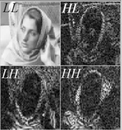
₁ .

The DWT, like the DCT, produces real valued coefficients. However, in image coding applications it is common to use the integer-to-integer mappings of the transforms, which can be done by rounding and truncating the transform coefficients [19]. In image coding, the DWT is applied to the all image region. The one level image analysis with DWT provides four subsets of coefficients organized in

sub-bands, as presented in figure 2. Sub-band

LL

corresponds to the lower frequencies (approximation coefficients), and sub-band

HH

corresponds to the higher frequencies (detail coefficients); the other sub-bands are intermediate frequency sub-bands.

Fig. 2 – One level image analysis with the DWT 2D.

In a multilevel image decomposition scheme there are hierarchical dependencies for each sub-band that must be taken into account to the scanning order of the coefficients. Figure 3 shows the dependencies of the DWT coefficients for a 3 level decomposition scheme.

Fig. 3 – Hierarchical sub-band relations of the DWT coefficients in a 3 level (L=3) image analysis scheme.

2.3 The S Transform

The S transform is one of the simplest and reversible transforms, also well known as the basic building block for the reversible integer-to-integer version of the DWT when using the Haar wavelet [9]. The appliance of the S transform to sequences is much like the DWT, with the particularity that it applies to pairs of pixels/coefficients: the even and odd ordered ones. The forward S transform maps a vector

[

x x

₀

,

₁

]

T to another vector

[

y y

₀

,

₁

]

T and is defined as

(

)

0 0 1 1 0 1 0.5 y x x y x x  ⋅ +    =     ₋     (5)

As in the DWT case, the direct S transform also has an integer-to-integer version, which is defined in equation (6), and achieved in a very simple way, by simple rounding and truncation operations after choosing the appropriate rounding operator [9].

1 0 0 1 1 , where 2 t x y t x x y t  ₊    ₌  _{ } _{= −}       _ _ (6) The corresponding inverse transform is defined by

0 1 1 0 1 , where 2 x y s y s y x s +   ₌  _{= −}    _ _  _{ }   (7)

The appliance of the S transform to image analysis is similar to the DWT case and, therefore, there is no need on further comments.

2.4 Measures for Coding Efficiency and Image Quality Evaluation

In this paper, in order to evaluate coding efficiency and image quality, we use the common parameters used for that purpose such as the compression ratio, the bit rate needed, and the peak signal to noise ratio (PSNR) obtained for the luminance component of the coded images. We also use other subjective evaluation criteria, by observing the coded images and comparing them with the original ones. The later criteria, due to its subjective dependence, should be done with a significant number of observers with different eye characteristics, in order to create a robust model. However, this task involves some requirements and logistics that we could not handle easily. Therefore, in this particular method, we simply consider the information provided by three different observers with different vision characteristics.

To evaluate the coding efficiency, we use the compression ratio defined as the ratio between the size of the original image file (the original signal) and the coded image file, as shown in equation (8).

O C

S S

γ = ₍₈₎

In image coding one also uses to measure the coding efficiency through the number of bits required for image transmission, considering the image size, usually expressed in bits per pixel (bpp).

The PSNR is defined by equation (9) where

A

represents the maximum pixel magnitude, (e.g.

255

A= for images with pixels represented by 8

bits), and MSE stands for the mean square error, defined in equation (10). 2 10 10 log A PSNR MSE = (9) 2 1 1 ( , ) ( , ) M N m n I m n I m n MSE M N ∗ = =  −    = ⋅

∑∑

₍₁₀₎

In equation (10)

M N

,

are the image dimensions,

( , )

I m n

refers to the pixel at position

( , )

m n

in the original image, and

I m n

∗

( , )

to the pixel with the same spatial coordinates in the coded image.

3 Structures of the Codecs Evaluated

This section presents the structures and describes the Codecs evaluated in this paper. We developed and evaluated five transform based image codecs: four JPEG-like image codecs and a EZW image coder. Due to its similarity in terms of structure (JPEG-like), in the first four codecs we group the following: a JPEG Baseline (DCT based), a JPEG DWT based [20], a JPEG DWT with Visual Threshold [21] and a JPEG ST based codec. The EZW image codec, which is DWT based, is presented separately due to its characteristics and also due to its differences to JPEG like codecs. Among the various studies concerning the use of DWT to image coding we refer in particular the work from Antonini et. al. [22], concluding that biorthogonal wavelet (4.4), also known as 9/7 filter pair, leads to the best results in image coding. The 9/7 wavelet filter pair is widely used in wavelet based image coding, mainly because of its good characteristics in minimizing phase distortion. The 9/7 filter pair is also used in all DWT based image codecs considered in this work.

For all the JPEG-like coders considered in this paper, i. e., JPEG Baseline, JPEG–DWT, JPEG–VT and JPEG–ST, the entropy coding block is Huffman coding. The Huffman tables used in all JPEG–like coders are those of JPEG Baseline Codec. For the EZW coder we use arithmetic coding in the entropy coding block.

3.1 JPEG Baseline

The structure of the transform based image coders is well known. Although the transform application, it also includes coefficient scanning, quantization and entropy coding. In this kind of image coders the JPEG Baseline is the simplest and the most popular, whose functional diagram is presented in figure 4.

Fig. 4 – Functional diagram of JPEG Baseline encoding.

The DCT is applied to blocks of 8x8 pixels in non-interlaced raster mode. According to the spatial organization of the DCT coefficients, its scanning order must take into account its significance. In DCT based image coding schemes, e.g JPEG Baseline, the scanning order of the transform coefficients is made in zig-zag, like it is shown in figure 5. The first coefficient is the lowest frequency coefficient, i.e. DC coefficient, and is scanned and quantized alone.

Fig. 5 – Scanning order of the DCT coefficients inside the block of 8x8 pixels.

The DCT coefficients are quantized using the quantization tables 1 and 2, for the luminance and chrominance components, respectively, as defined for JPEG standard.

                          99 103 100 112 98 95 92 72 101 120 121 103 87 78 64 49 92 113 104 81 64 55 35 24 77 103 109 68 56 37 22 18 62 80 87 51 29 22 17 14 56 69 57 40 24 16 13 14 55 60 58 26 19 14 12 12 61 51 40 24 16 10 11 16

Tab. 1 – Luminance coefficients quantization table.

                          99 99 99 99 99 99 99 99 99 99 99 99 99 99 99 99 99 99 99 99 99 99 99 99 99 99 99 99 99 99 99 99 99 99 99 99 99 99 66 47 99 99 99 99 99 56 26 24 99 99 99 99 66 26 21 18 99 99 99 99 47 24 18 17

Tab. 2 – Chrominance coefficients quantization table.

The Huffman coding [23] block is an entropy coding process, which is based on tables that respect the probabilities of occurrence of the coefficients, and that are also linked to the nature of the coefficients, i.e., the low and high frequencies coefficients of the luminance and the chrominance components, etc.

3.2 JPEG–DWT

More recently there has been a growing interest on the use of wavelets in image coding schemes. Several authors have studied the application of the DWT to image coding. However, although the superior performance achieved with relation to most of JPEG coders, the application of the DWT often leads to higher complexity coding schemes. In order to minimize the coding complexity when using the DWT, Queiroz et. al. proposed a JPEG-like image coder based on the DWT [20]: the JPEG-DWT coder, which structure is presented in figure 6.

Fig. 6 – Structure of the JPEG–DWT coder (based on the typical JPEG structure).

As one can observe, the structure of the JPEG– DWT coder is very similar to that of the JPEG Baseline. As a main difference one has to mention the use of the DWT instead of the DCT; the DWT is applied to the all image region with 3 levels of decomposition.

Regarding the hierarchical relations of the coefficients of the DWT (see fig. 3), one has to consider modifications to the scanning order of the

block of 8x8 coefficients, respecting its locations in the frequency bands, and its dependencies. To do this one has to form blocks of 8x8 coefficients (like as in the JPEG coder), whose coefficients are organized as depicted in figure 7.

After the formation of each 8x8 block, one must perform a modified scanning order of the block coefficients as depicted in figure 8. The coefficients in the same relative location, in different sub-bands, are grouped together in the same block.

Fig. 7 – Procedure for the block construction of 3-level DWT coefficients, for the JPEG–DWT coder.

For a 3 level DWT decomposition, this scheme fits perfectly into a block of 8x8 coefficients₍₂3_=8).

Fig. 8 – Modified scanning order in the constructed block of 8x8 coefficients of the 3 level DWT.

In JPEG Baseline the quantization table has 64 entries representing uniform quantization steps. For the JPEG–DWT coder with 3 levels of

decomposition (L=3), we consider the model

defined in [20] to average the quantizer steps for all the coefficients in the same subband, with respect to a variable

A

to control the bit rate.

For A=6.7, and 3 levels of decomposition, one obtains the quantization matrix in table 3 [20].

                          55 55 55 55 34 34 34 34 55 55 55 55 34 34 34 34 55 55 55 55 34 34 34 34 55 55 55 55 34 34 34 34 34 34 34 34 12 12 8 8 34 34 34 34 12 12 8 8 34 34 34 34 8 8 7 7 34 34 34 34 8 8 7 8

Tab. 3 – Quantization table for the 3 analysis levels.

3.3 JPEG–DWT with Visual Threshold

Often, to achieve better compression results, one leads to higher loss values and also on a significant increase on computational complexity, thus sacrificing performance. In order to get good compression results without having great losses and avoiding poor performance, some special coding techniques were developed, based on the perceptual characteristics of the HVS, also known as “perceptual compression techniques”. The JPEG – DWT coder with Visual Threshold (JPEG VT) has a structure similar to that of the JPEG-DWT mentioned in the previous section, and is based on visual measures with different threshold values. The measures were taken for different observers, according to models in the YCbCr space [21].

According to [21], the quantization steps in JPEG-DWT coder with visual thresholds depends on the spatial localization of the coefficients, on the number of decomposition levels of the DWT, and also on the image component (Y,Cb,Cr) and the observing angle. Also as established in [21], the quantization of the transform coefficients is supported in a mathematical model based on experimental results with various observers, whose results are shown in table 4.

Level of Analysis Image Comp. Sub-band

1 2 3 LL 14.049 11.106 11.363 HL 23.028 14.685 12.707 LH 23.028 14.685 12.707

Y

HH 58.756 28.408 19.540 LL 55.249 46.559 48.450 HL 86.789 60.485 54.571 LH 86.789 60.485 54.571

Cb

HH 215.84 117.45 86.737 LL 25.044 19.282 19.665 HL 60.019 34.335 27.276 LH 60.019 34.335 27.276

Cr

HH 184.64 77.569 47.441

Tab. 4 – Quantization factors for the DWT with 9/7 filter pair, with 3 analysis levels, according to the image components and sub-band location of the coefficients (extracted from [21]).

3.4 JPEG – ST

The structure of the JPEG–ST coder is also similar to the structure of the simple JPEG-DWT. The main difference is the type of transform used; all the other coding blocks remain unchanged, i. e., the formation of the blocks, the quantization process, and the Huffman coding are similar to those of JPEG –DWT coder.

3.5 EZW Coder

One knows that information in natural images is predominant at low frequency components. On the other hand, the DWT characteristics in image analysis tends to concentrate energy in lower bands (higher levels), thus, the coefficients located at the higher levels of decomposition are more significant than those located in lower levels. The significance of the coefficients decreases as the level decreases inside the transformed image.

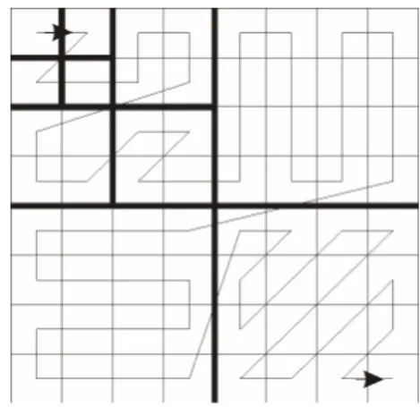
The EZW coding scheme [13] is strongly based in the high probability that the coefficients of the 2D structure of the decomposed image, at the higher levels (lower bands), are more significant than those located at lower levels (higher bands). The significance of the coefficients decreases as the level decreases inside the image. The scanning order of the coefficients is fixed, assuring that the coefficients located in the higher levels are scanned prior to those located at the lower levels. This is performed form higher to lower levels, taking into account the dependencies of the coefficients in the tree, as depicted in figure 9.

Fig. 9 – Scanning order of the DWT coefficients in EZW

In two dimensions, a node at the first level of the pyramid, also called root of the tree, or root node, has three children nodes, a node at the middle level or, intermediate level, has four children while a node at the bottom of the tree (leaf node) has no children. For images with dimensionM N× , with p levels of

decomposition, the dimensions of the tree root region are defined by Mh×Nh, where

2 h p M M = and 2 h p N

N = . We refer the subsets of DWT coefficients

in the tree-root, in an intermediate level and the coefficients located in the bottom level by, R, I and

B, respectively. Referencing each coefficient by its coordinates( , )m n , one can state the parent-children linkage [24], or hierarchical dependencies of the tree structure as, { h h h h} m n → m M n+ m n N+ m M n N+ + m n ∈ ( , ) ( , ),( , ),( , ) if ( , ) R { } m n → m n m+ n m n+ m+ n+ l m n∈ ( , ) (2 , 2 ),(2 1, 2 ),(2 , 2 1),(2 1, 2 1) if ( , , ) I { } m n → m n ∈ ( , ) if ( , ) B

With reference to a threshold, four symbols are used: positive or POS (if the coefficient is found significant and positive); negative or NEG (if the coefficient is found significant and negative); zero-tree-root, or ZTR (if the coefficient is found insignificant, also as all its dependents) and isolated zero or IZ (if the coefficient is insignificant but there are coefficients dependents that are significant). The initial threshold value,

T

₀, is set to a power of 2, not greater neither equal to the maximum absolute value of the coefficients in the matrix, as defined in equation (11).

( ) ( )

(

)

2 log max , 0 2 x y T ₌  γ   ₍₁₁₎

During EZW coding two lists are maintained: a dominant list, which is of first-in first-out type (FIFO), and a subordinate list. In the dominant pass, the coefficients are scanned, and significant coefficients are coded, which corresponds to add their value and coordinates to the dominant list, and to fill with zero the corresponding position in the matrix (preventing from coding in a future dominant pass), otherwise it remains unchanged to the next dominant pass. After the dominant pass a subordinate pass is performed in order to refine the coding, using a threshold value that is half of the one used in the dominant pass. After completing each pair of dominant and subordinate passes, the threshold is halved, and a new scanning and coding process restarts.

Due to the unavailability of Huffman tables best suited for this type of coder, we use arithmetic coding in the entropy coding block.

4 Evaluation Results and Comments

The codecs described in the previous sections were implemented in MATLAB™. Test images such as

“Lena”, “Airplane” and “Baboon” with spatial resolutions of 128x128, 256x256 and 512x512 were coded, in order to evaluate the performance of the codecs and the quality of the coded images. To avoid degradation at the bound regions of the images due to the zero fill of initial conditions, in DWT calculations, the sequences were symmetrically extended [25], and the extended coefficients are finally discharged, in order to maintain in-place computation. To evaluate of the quality of the coded images we consider the compression ratio, the bit-rate, and PSNR. We also consider subjective quality evaluation by visual inspection.

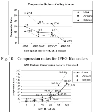
Figures 10 to 13 show compression ratios and bit rates obtained for JPEG-like coders, and for EZW coders. For JPEG–like coders, compression ratios vary from approximately 2 to 27, and bit rates vary from 0.11 to 1.5 bpp. The best results are obtained for JPEG Baseline; similar results ate obtained for JPEG DWT and for JPEG VT, and the worst results are obtained for JPEG–ST. However, is this last case, although the poor results obtained for compression ratio and bit rate, we must refer its simplicity of implementation. For the EZW coders, compression ratios vary from 5 to 185, approximately and bit rates vary form 0.02 to 1.46 bpp, depending on the threshold used. The best results are obtained for “Lena” image and the worst results for “Baboon”. This is due to the characteristics of these images, as “Baboon” has too many details, rather than “Lena”.

Compression Ratio vs . Coding S cheme

2,05 17.6 17.9 27.3 9.9 15 9.2 6 10.9 7.9 0 5 10 15 20 25 30

JPEG JPEG DWT JPEG VT JPEG ST Coding Scheme for 512x512 Image s

Co m pr es si on Ra ti o Lena Airplane Baboon

Fig. 10 – Compression ratios for JPEG-like coders

EZW Coding: Compression Ratio vs. Threshold 185.84 107.64 58.46 29.17 5.17 115.13 59.35 29.82 120.82 50.19 18.23 7.05 0 20 40 60 80 100 120 140 160 180 200 4 8 16 32 64 128

EZW Thre shold

Co m pr es si on Ra ti o Lena Airplane Baboon

Bit-Rate vs . Coding S cheme 0 0,2 0,4 0,6 0,8 1 1,2 1,4 1,6

JPEG JPEG DWT JPEG VT JPEG ST

Coding Sche me for 512x512 Image s

B it -R ate [b pp ] Lena Airplane Baboon

Fig. 12 – Bitrate (in bits per pixel), for JPEG-like coders

EZW Coding: Bit-Rate vs . Threshold

0.57 0.22 0.1 1.46 0.8 0.34 0.13 0.05 0.02 0 0,2 0,4 0,6 0,8 1 1,2 1,4 1,6 4 8 16 32 64 128

EZW Thre shold

B it -R at e [ bpp] Lena Airplane Baboon

Fig. 13 – Bitrate (in bits per pixel), for EZW coding

Figures 14 and 15 show PSNR results for JPEG-like for EZW coders. For the same image similar PSNR results are obtained with the various JPEG–like coders, with maximum differences of 2 to 3 dB approximately. For EZW coders we obtain values of PSNR from 17 to 34 dB (approx.). PSNR varies 3 to 4 dB when the threshold is halved. However, for threshold 128, although the coded images can maintain some intelligibility, the visual quality is in general very poor, and therefore, due to the high losses registered we do not consider it so efficient.

Peak S ignal to Noise Ratio vs . Coding S cheme

27 32.14 30.8 33 34.8 25 _25.4 28.15 10 15 20 25 30 35 40

JPEG JPEG DWT JPEG VT JPEG ST

Coding Scheme for 512x512 Image s

PS N R [ dB ] Lena Airplane Baboon

Fig. 14 – Curves of PSNR for the JPEG-like coders

EZW Coding: PS NR vs . Threshold

19 17 23.78 28.1 31.86 35.18 39.37 20.3 23.3 26.6 30.12 34.19 10 15 20 25 30 35 40 45 4 8 16 32 64 128

EZW Thre shold

PS N R [ dB ] Lena Airplane Baboon

Fig. 15 – Curves of PSNR for EZW coding with different threshold values.

In figures 16 and 17 we show the variations of PSNR and bit rate for different coders, considering “Lena” and “Airplane” images, respectively. From this figures one can observe that JPEG DWT and JPEG DWT with Visual Thresholds perform similar, that JPEG Baseline performs similar than EZW coder with threshold 16, and that EZW with thresholds 32 and 64 perform considerably better than the other coders, considering a reasonable degree of intelligibility in the coded images, taken by observation.

Evaluation for Bitrate and PS NR vs . Coding S cheme for "Lena" 512x512 0,00 0,02 0,04 0,06 0,08 0,10 0,12 0,14 0,16 0,18 0,20

J PEG J PEG DWT J PEG VT EZW16 EZW3 2 EZW6 4 Coding Sche me bi tr at e [ bpp] 0 5 10 15 20 25 30 35 40 P SNR [ dB ] bpp PSNR

Fig. 16 –Performance of JPEG-like coders for “Lena”

Evaluation for bitrate and PS NR vs. Coding S cheme for "Airplane" 512x512 0,00 0,02 0,04 0,06 0,08 0,10 0,12 0,14 0,16 0,18 0,20

J PEG J PEG DWT J PEG VT EZW16 EZW3 2 EZW6 4 Coding Sche me bi tr at e [b pp ] 0 5 10 15 20 25 30 35 40 PS N R [ dB ] bpp PSNR

Fig. 17 – Performance of JPEG-like coders for “Airplane”

5 Conclusions

This paper addresses the evaluation of image coding schemes, with particular interest in image coding schemes that use other transforms rather than DCT, namely the wavelet transform and the S transform. The DWT and the ST are applied in the space domain using, using the 9/7 wavelet filter pair in the case of DWT based coders. Compression ratios, bit rate values and PSNR were presented in order to allow codec evaluation in performance, and quality analysis of the coded images. From the experimental results obtained, and also from subjective information taken by observation, one can conclude that in general the DWT based coders perform better than JPEG Baseline. The JPEG coder with Visual Threshold technique, in general, has no relevant differences to the simple JPEG DWT, so we conclude that although the subjective dependencies of the Visual Threshold technique, there are no significant benefits and therefore it is not so

important. For similar compression ratios, the EZW coder outperforms all the other codecs in terms of compression ration, bit rate and PSNR. However, the EZW coder is the most complex in terms of implementation, while the DWT ST is the simplest. Also one must notice the scalability properties of the EZW coding scheme, which has particular interest in image transmission.

References:

[1] J. D. Gibson, T. Berger, T. Lookabaugh, D. Lindbergh, R. Baker, Digital Compression for

Multimedia, Morgan Kaufmann Publishers, 1998

[2] V. K. Madisetti, D. B. Williams, The Digital

Signal Processing Handbook, CRC Press/ IEEE

Press, 1998.

[3] V. Baskaran, K. Konstantinides, Image and

Video Compression Standards, Kluwer

Academic Press, 2nd _{Ed, 1996.}

[4] R. Gonzalez, R. Woods, Digital Image

Processing, Addison–Wesley Publishing, 1993.

[5] J. S. Lim, Two Dimensional Signal and Image

Processing, Prentice-Hall, 1990.

[6] K. N. Plataniotis, A. N. Venetsanapoulos, Color

Image Processing and Applications, Springer,

2000.

[7] G. Strang, “The Discrete Cosine Transform”,

SIAM Review, 41, 1999, pp. 135 – 147.

[8] I. Daubechies, Ten Lectures on Wavelets, SIAM – Society for Industrial and Applied Mathematics, 1992.

[9] M. D. Adams, F. Kossentini, R. K. Ward, “Generalized S Transform”, IEEE Transactions

on Signal Processing, Vol. 50, N. 11, November

2002, pp. 2831 – 2842.

[10] G. Sharma, H. J. Trussel, “Digital Color Imaging”, IEEE Trans. on Image Processing, Vol. 6, N. 7, July 1997, pp. 901 – 932.

[11] G. K. Wallace, “The JPEG Still Picture Compression Standard”, IEEE Transactions on

Consumer Electronics, Vol. 38, Issue 1,

February 1992, pp. xviii – xxxiv.

[12] W. A. Pearlman, A. Said, “A Survey on State-of-the-Art and Utilization of Embbeded Tree-Based Coding”, Proceedings of IEEE Int. Symp.

On Circuits and Systems, Invited Paper,

Monterey, Canada, June 1998.

[13] J. M. Shapiro, “Embedded Image Coding Using Zero-trees of Wavelet Coefficients”, IEEE

Transactions on Signal Processing, Vol. 41, N.

12, December 1993, pp. 3445 – 3462.

[14] A. Said, W. A. Pearlman, “A New, Fast, and Efficient Image Codec Based on Set Partition in Hierarchical Trees”, IEEE Transactions on

Circuits and Systems for Video Technology, Vol.

6, N. 3, June 11996, pp. 243 – 250.

[15] D. Taubman, “High Performance Scalable Image Compression with EBCOT”, IEEE

Transactions on Image Processing, Vol. 9, N. 7,

July 2000, pp. 1158 – 1170.

[16] A. Skodras, C. Christopoulos, T. Ebrahimi, “The JPEG 2000 Still Image Compression Standard”, IEEE Signal Processing Magazine, Vol. 18, N. 5, September 2001, pp. 36 – 58. [17] B. E. Usevitch, “A Tutorial on Modern Lossy

Wavelet Image Compression: Foundations of JPEG 2000”, IEEE Signal Processing Magazine, Vol. 18, N. 5, September 2000, pp. 22 – 35. [18] M. Vetterli, C. Herley, “Wavelets and Filter

Banks: Theory and Design”, IEEE Transactions

on Signal Processing, Vol. 40, Issue 9,

September 1992, pp. 2207 – 2232.

[19] A. R. Calderbank, I. Daubechies, W. Sweldens, B. L. Yeo, “Wavelets Transforms that Map

Integers to Integers”, Applied and

Computational Harmonic Analysis Journal, Vol.

5, N. 3, 1998, pp. 332 – 369.

[20] R. Queiroz, C. K. Choi, Y. Huh, K. R. Rao, “Wavelets Transforms in a JPEG-Like Image Coder”, IEEE Transactions on Circuits and

Systems for Video Technology, Vol. 7, N. 2,

April 1997, pp. 419 – 424.

[21] A. B. Watson, G. Y. Yang, J. A. Solomon, J. Villasenor, “Visual Thresholds for Wavelet Quantization Error”, Proceedings of the SPIE, Vol. 2657, Human Vision and Electronic Imaging, The Society for Imaging Science and Technology (1996).

[22] M. Antonini, M. Barlaud, P. Mathieu, I. Daubechies, “Image Coding using Wavelet Transform”, IEEE Trans. on Image Processing, Vol. 1, N. 2, April 1992, pp. 205 – 220.

[23] David A. Huffman, “A Method for the Construction of Minimum-Redundancy Codes”,

Proceedings of the I.R.E, Vol. 40, September

1952, pp. 1098 – 1101.

[24] Y. Chen, W. A. Pearlman, “Three-Dimensional Subband Coding of Video Using the Zero-Tree Method”, Proceedings of the SPIE’s 1996

Symposium on Visual Communications and Image Processing, Vol. 2727, March 1996.

[25] C. Brislawn, “Classification of Nonexpansive Symmetric Extension Transforms for Multirate Filter Banks”, Applied and Computational

Harmonic Analysis, Vol. 3, N.3, 1993, pp. 148–