___________________________________________
1Engº Agrícola, Prof. Doutor, Centro de Ecofisiologia e Biofísica, Instituto Agronômico/Campinas – SP, Fone: (19) 2131-0612,
Recebido pelo Conselho Editorial em: 17-1-2013
OF SÃO PAULO-BRAZIL: AN STUDY BASED ON THE EXTREME VALUE THEORY
GABRIEL C. BLAIN1
ABSTRACT: The application of the Extreme Value Theory (EVT) to model the probability of
occurrence of extreme low Standardized Precipitation Index (SPI) values leads to an increase of the knowledge related to the occurrence of extreme dry months. This sort of analysis can be carried out by means of two approaches: the block maxima (BM; associated with the General Extreme Value distribution) and the peaks-over-threshold (POT; associated with the Generalized Pareto distribution). Each of these procedures has its own advantages and drawbacks. Thus, the main goal of this study is to compare the performance of BM and POT in characterizing the probability of occurrence of extreme dry SPI values obtained from the weather station of Ribeirão Preto-SP (1937-2012). According to the goodness-of-fit tests, both BM and POT can be used to assess the probability of occurrence of the aforementioned extreme dry SPI monthly values. However, the scalar measures of accuracy and the return level plots indicate that POT provides the best fit distribution. The study also indicated that the uncertainties in the parameters estimates of a probabilistic model should be taken into account when the probability associated with a severe/extreme dry event is under analysis.
KEYWORDS:Extreme Value distribution, Pareto distribution, goodness-of-fit tests.
TEORIA DOS VALORES EXTREMOS APLICADA À OCORRÊNCIA DE MESES SECOS EM UMA REGIÃO AGRÍCOLA DO ESTADO DE SÃO PAULO
RESUMO: A aplicação da Teoria dos Valores Extremos (EVT) para modelar a probabilidade de
ocorrência dos extremos inferiores do Índice Padronizado de Precipitação (SPI) leva ao aprofundamento do conhecimento relativo à ocorrência de meses secos. Esse tipo de análise pode ser realizado com base nos métodos dos máximos em bloco (BM; associado à distribuição Geral
dos Valores Extremos) e dos peaks-over-threshold (POT; associado à distribuição Pareto
Generalizada). Considerando que cada um desses procedimentos apresenta vantagens e desvantagens, o objetivo principal do trabalho foi comparar o desempenho de ambos os métodos na caracterização da probabilidade de ocorrência dos extremos secos do SPI obtidos a partir da estação meteorológica de Ribeirão Preto-SP (1937-2012). De acordo com os testes de aderência, o BM e o POT podem ser usados para avaliar a probabilidade de ocorrência de valores mensais extremamente secos do SPI obtidos na referida localidade. Entretanto, medidas escalares de precisão e gráficos de nível de returno indicam que o POT resulta no melhor ajuste. O estudo também demonstrou que as incertezas na estimação dos parâmetros de modelos probabilísticos devem ser consideradas quando a probabilidade de ocorrência dos eventos em análise estiver sendo avaliada.
PALAVRAS-CHAVE:Distribuição de valores extremos, distribuição Pareto, testes de aderência,
INTRODUCTION
Precipitation Index (SPI1) is a probability-based procedure developed for characterizing rainfall departures with regard to an expected local climate condition (GUTTMAN, 1999; BORDI et al., 2007; SANTOS et al., 2011 and BLAIN, 2012a, among others). Consequently, the SPI is suitable for detecting a shortage of water supply especially during those months in which high precipitation amounts are expected (BLAIN 2012a,b). As can be noted from the SPI calculation algorithm (BLAIN, 2012a), for those locations with a distinctly dry season, the lowest (or driest) SPI values tend to be observed during the rainy season. Moreover, according to BORDI et al. (2007) and HAYES et al. (2011), we may assume that the characterization of a dry event does not rely entirely on low precipitation amounts; it also depends on a negative anomaly of these amounts with respect to an expected local climate condition (BORDI et al., 2007). This last feature may be seen as one of the reasons that lead the SPI to be widely used by governmental agricultural institutions, such as
Empresa Brasileira de Pesquisa Agropecuária (EMBRAPA), Instituto Agronômico (IAC) and Instituto Nacional de Meteorologia (INMET).
According to SANTOS et al. (2011) an important task in drought risk evaluation is to assess the rarity of severe dry events. Hence, assessing the probability of occurrence of extreme low SPI values leads to an increase of the knowledge related to the occurrence of extreme dry months. After BORDI et al. (2007) have stated that the SPI is more suitable than the rainfall for charactering
extreme dry monthly events they used the Extreme Value Theory (EVT) to model the probability of
extreme dry periods in Sicily-Italy.
A question that arises when an extreme value analysis is being carried out is related to what should be regarded as an extreme event (WILKS, 2011). A practical decision is to adopt the so-called block maxima or minima approach (BM), in which the blocks are considered equal to one year. The BM selects the largest (or the smallest) single value in each year or block (WILKS, 2011).
A desirable feature of the use of the BM is that it removes the influence of serial correlations on the estimates. However, this procedure also leads to a large loss of information (or data) by sampling only one value from each block (the average sample rate of the BM is equal to 1 event per
year; λ=1). To overcome this undesirable feature one may adopt the procedure called
peaks-over-threshold (POT). According to SUGAHARA et al. (2009) the abovementioned large loss of data has been an important reason for the increasing use of the POT. This last approach selects any value larger than (or smaller than) a threshold regardless of their year of occurrence (WILKS, 2011). The asymptotic distribution of a dataset that was correctly sampled by the POT is the Generalized Pareto Distribution (GPD) (COLES, 2001, SUGAHARA et al., 2009, KATZ, 2010 and WILKS, 2011). Naturally, a dataset can only be correctly sampled by the POT if an appropriate threshold is chosen. As described by COLES (2001), a too low threshold may violate the asymptotic basis of the function, leading to bias. On the other hand, a too high threshold may lead to a great loss of data resulting in high variance of the parameters estimations. SUGAHARA et al. (2009) state that choosing an appropriate threshold is a fundamental step for using the POT. At this point, we may pose the same question presented in WILKS (2011): Which of these approaches (BM or POT) is more useful for a given application? According to authors such as MADSEN et al. (1997) this question should be empirically evaluated for each location under analysis.
The aforementioned arguments, associated with the fact that a severe/extreme rainfall deficit frequently leads to crop yield reductions (BACK & UGGIONI, 2010), have motivated us to verify (i) whether the BM and/or POT can be used to assess the probability of occurrence of extreme dry SPI values in an agricultural region of the State of São Paulo, Brazil and (ii) which of these approaches provides the best characterization of the probability of occurrence of extreme dry months. Thus, the goals of this study were to apply both BM and POT to sample the extreme SPI data, obtained from the weather station of Ribeirão Preto (1937-2012), and to empirically compare the performance of these both approaches in providing the best fit extreme value distribution. It is
1 Developed by Mckee, T.B.; Doesken, N.J.; Kleist, J. and first presented at the 8th Conference on applied climatology (1993) of the
expected that this study should provide a better assessment of the probability of occurrence of extreme dry months that may be linked to crop yield reductions.
MATERIAL AND METHODS
Monthly rainfall totals were obtained from the weather station of Ribeirão Preto (21º11’S,
47º48’W, 620m – 1937 to 2012; State of São Paulo, Brazil). As can be noted from studies such as
BLAIN (2009) the shape of these monthly probability functions vary from a strongly skewed distribution similar to those observed in arid climate (July) to a bell-shaped distribution similar to those observed in equatorial climate (January). All statistical tests of this study were performed at the 5% significance level.
As described by GUTTMAN (1999) the SPI calculation starts by determining a parametric distribution (cdf[x]) capable of properly describing the long-term observed precipitation. According to BLAIN (2011, 2012b), the rainfall monthly series of Ribeirão Preto can be considered as coming from a 2-parameter gamma distribution or a 3-parameter Pearson Type-III distribution (PE3). The cumulative probability [H(PRE)], associated with a given rainfall amount, is obtained from the following mixed distribution (equation 1) where m is the number of zeros observed in a dataset
composed by N observations.
) ( )] / ( 1 [ ) / ( )
(PRE m N m N cdf x
H (1)
The final step of the SPI calculation algorithm is to subject H(PRE) to an equiprobabilistic transformation. This last step aims to transform H(PRE) into a normally distributed process with zero mean and unit variance. The SPI (dry) categories are shown in Table 1.
TABLE 1. The SPI classification system.
SPI values Category
−1.00 to −1.49 Moderately dry
−1.50 to −1.99 Severely dry
Less than −2.00 Extremely dry
Note. Extracted from GUTTMAN (1999)
Based on distinct locations of the State of São Paulo, BLAIN (2011) has indicated that the SPI series obtained from the PE3 meets more frequently the normality assumption (intrinsic to the use of this standardized index) than the SPI series obtained from the gamma. Therefore, we estimated the SPI monthly values by using the PE3 distribution (GUTTMAN, 1999, SANTOS et al., 2010, BLAIN, 2011 and BLAIN, 2012b).
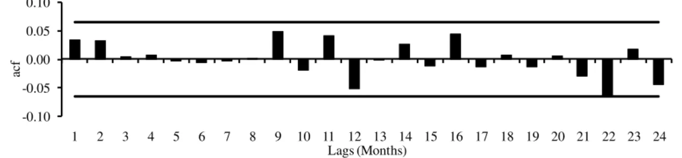
Finally, it is worth emphasizing that the SPI can be calculated for several time scales. However, as described in BORDI et al. (2007), time scales greater than the monthly scale introduces temporal persistence or serial correlations into its series. These authors state that the presence of a significant serial correlation is an undesirable feature for applying the EVT. Thus, we decided to estimate the SPI only at the monthly scale. The presence of serial correlation in the SPI monthly series was evaluated by using the autocorrelation function (acf; WILKS, 2011).The acf coefficients were estimated up to lag 24 (months). Although the number of lags (#Lags) is an
arbitrary choice, the upper limit #Lags ≤ N/4 was respected.
Block maxima and Peaks-over-threshold
The Extremal Types Theorem implies that when the highest values of a process are stabilized
COLES (2001), each one of these three different types of distributions gives distinct representations of extreme value behavior. Therefore, in some applications of the EVT, it is usual to adopt, at least, one of these types, and then to estimate the parameters of the adopted function. Naturally, a technique should be applied to select the most appropriate type for each data sample (COLES, 2001). Fortunately, these three types can be combined into a single function; the General Extreme Value Distribution (GEV; equation 2 in its cumulative form). By using the GEV function, the data
themselves specify the most appropriate type of tail behavior and there is no need to make a priori
judgments about which individual type (Gumbel, Fréchet or Weibull) should be adopted (COLES, 2001). 1/ ) PI ( 1 exp GEV(SPI) S (2)
The parameters of the GEV distribution were estimated by using the method of maximum likelihood (ML) as described in several studies such as Coles (2001), WILKS (2011), FURIÓ & MENEU (2010) and BLAIN & CAMARGO (2012). Hereafter, these estimative will be represented by the following characters: μ (location), σ (scale), ξ (shape) and, for the sake of brevity, will be
referred to as parameters. As described in studies such as DELGADO et al. (2010), while σ defines
the spread of the distributions, μ defines the position of the GEV function with regard to the origin.
The Gumbel distribution corresponds to the case ξ=0. The Fréchet and Weibull distributions
correspond, respectively, to the cases ξ>0 and ξ<0 (COLES, 2001). According to CANNON (2010)
ξ is the main determinant of the tail behavior.
SUGAHARA et al. (2009) observed that several strategies have been proposed for selecting an appropriate threshold for using the GPD (equation 3, in its cumulative form). However, according to these authors, the scientific literature still lacks of a general and objective method to define such a threshold. In this study, the threshold was selected by means of two different procedures described in COLES (2001). The first one, called mean residual life plot, is an exploratory method that is based on the mean of the GPD in the sense that the expectation E(SPI-threshold|SPI>threshold) is a linear function of all valid thresholds. The second one is based on the search of stability of the parameters estimations obtained by adopting different thresholds. Further information regarding these two procedures can be found in COLES (2001). The parameters of the GPD distribution were also estimated by using the ML, which is frequently regarded as a robust parameter estimation procedure (HADDAD & RAHMAN, 2010).
1 * 1 1 ) ( SPI threshold
SPI
GPD (3)
Goodness-of-fit
The chi-square test (χ2) and the Kolmogorov-Smirnov test (KS) are often used to check the fit
of a given data sample to a parametric distribution (WILKS, 2011). The χ2 is suitable for discrete
random variables because to calculate it, the range of the data must be divided into discrete classes (WILKS, 2011). On the other hand, the KS test compares the theoretical and the empirical cumulative distribution. Hence, for continuous data such as the SPI, the KS test tends to be more
powerful than the χ2 (WILKS, 2011). The null hypothesis (H
0) of the KS test states that the data was drawn from the theoretical distribution under analysis. However, according to authors such as
WILKS (2011) and VLČEK & HUTH (2009) the original KS calculation algorithm is applicable if,
and only if, the parameters of the theoretical distribution have not been estimated from the same sample used to evaluate the fit of the parametric distribution.
Given that the parameters of the extreme value distributions were fitted using all available data, the KS test had to be modified. This adapted method is frequently mentioned as Kolmogorov-Smirnov/Lilliefors test (KS-L; WILKS 2011). The statistical simulations required for its calculation
were based on the method called “non-uniform random number generation by inversion” as
Regarding extreme-value statistics, the Anderson-Darling (AD) test (equation 4) is based on the sum of the squares of the differences between theoretical and empirical distribution with a
weight function [Ψ(SPI)] which emphasizes the discrepancies in both upper and lower tails (SHIN
et al., 2012). This last feature cannot be observed in the KS-L algorithm.
N F SPI G SPI SPI dG SPI
Qn 2 (4)
where,
N = the length of the series, G(SPI) is the parametric cumulative distribution function, and
F(SPI) = the empirical distribution and Ψ(SPI) ={G(SPI)[1-G(SPI)]}-1.
According to SHIN et al. (2012) the AD test is a powerful test because it emphasizes the tails differences. However, one may correctly argue that equation 4 gives equal weights to both upper and lower tails of the distribution (SHIN et al., 2012). So, studies addressing drought events are naturally interested in the lower tail of the (SPI) distributions rather than in its upper tails. Thus, the
use of a Ψ(SPI) function that, for the present case, gives emphasis to discrepancies at the lower tails
of the distributions becomes an interesting choice. Considering this background, a modified form of the AD test (equation 5; AU) that gives emphasis to the lower tails of the distributions should also be used. As for the KS-L, the null hypothesis of the AU and AD were obtained by using the
procedure called “non-uniform random number generation by inversion” (Ns=10000).
SPI dG SPI
SPI G
SPI G SPI F N AU
1
2
(5)
After analyzing equations 4 and 5, one may correctly argue that a weakness of the AD and AU tests is that both F(SPI) and G(SPI) tend to 1 as the SPI absolute values increase. Naturally, the same weakness can be associated with the use of the KS-L test. According to COLES (2001), this deficiency can be avoided by analyzing the quantile estimation, which can be obtained by inverting equations 2 (QGEV) and 3 (QGPD). The mean absolute error (MAE) and the mean squared error
(MSE) were used to evaluate the agreement between these estimates (QGEV and QGPD) and the SPI
values. Further information regarding the MAE and the MSE can be found in WILKS (2011). Finally, the return level plot, as described in several studies such as COLES (2001), was used as a qualitative assessment of the goodness-of-fit of the two parametric models.
RESULTS AND DISCUSSION
-0.10 -0.05 0.00 0.05 0.10
1 2 3 4 5 6 7 8 9 10 11 12 13 14 15 16 17 18 19 20 21 22 23 24
acf
Lags (Months)
FIGURE 1. Auto-correlation function (acf) applied to the monthly SPI series of the location of Ribeirão Preto (1937-2012), SP.
Block maxima and Peaks-over-threshold
The mean residual life plot (not shown here for the sake of brevity) has indicated that the expectation E(SPI-threshold|SPI>threshold) may be seen as a linear function of threshold values equal to or smaller than -0.85. So, by adopting several thresholds values (raging from -2.0 to -0.5) it was observed that the parameters of equation 2 remains approximately constant for values equal to or smaller than -0.85. At this point, it is worth emphasizing that a threshold ≤ -0.85 leads to an average sample rate λ=2.10 events per year which is, naturally, greater than the sample rate obtained from the BM approach. Thus, by following the idea that a threshold must not result in the violation of the asymptotic basis of the GPD function and it also must avoid the great loss of data associated with the BM approach (COLES, 2001; BORDI et al., 2007;SUGAHARA et al., 2009 and WILKS, 2011), we adopted a threshold equal to -0.85, which is also virtually equal to the threshold (-0.84) used by SANTOS el al. (2011).
The parameters of the two distributions are: μ =1.213 [0.0688], σ=0.416 [0.0384], ξ=0.089 [0.0524]
(GEV); σ*=0.459 [0.0506], ξ=0.0636 [0.0762] (GPD); [.] represents the standard error associated with
each estimate. Positive values of the shape parameter imply that both distributions have no upper limit (COLES, 2001; WILKS, 2011). Considering that the rainfall distributions, from which the SPI values were calculated, have a physical lower limit associated with the zero value, these positive values of ξ
should be regarded as an indication that the real lower limit of the SPI distributions could not be specified. It also should be remembered that all SPI data were multiplied by -1.
Goodness-of-fit tests such as the KS-L, AD and AU provide empirical evidences for rejecting or accepting the null hypothesis that a given parametric distribution may be used to describe the probability of occurrence of a given variable. This last statement is based on the fact that these tests quantify the agreement between the empirical cumulative distribution and the theoretical cumulative function (WILKS 2011 and SHIN et al., 2012).
TABLE 2. Kolmogorov-Smirnov/Lilliefors (KS-L) test, Anderson-Darling test (AD), Modified Anderson-Darling test (AU), mean absolute error (MAE) and mean squared error (MSE) used to evaluate the fit of the General Extreme Value distribution (GEV) and the Generalized Pareto distribution (GPD) to the extreme dry SPI values obtained from the weather station of Ribeirão Preto-SP.
Model KS-L AD AU MAE MSE
GEV 0.073 (p-value =0.7) 0.418 (p-value =0.8) 0.171 (p-value =0.8) 0.08 0.03
GPD 0.055 (p-value =0.8) 0.438 (p-value =0.8) 0.252 (p-value =0.7) 0.04 0.01
Considering the 95% confidence interval, the visual analysis of Figure 2 clearly indicates that the GEV model is inconsistent with the most extremes SPI values obtained from the weather station of Ribeirão Preto. However, the same analysis indicates that the GPD model is consistent with all observed data. Thus, similar to what was indicated by the MAE and MSE, the results depicted in Figure 2 indicate that the GPD is better than the GEV for describing the probability associated with extreme dries SPI values obtained from the abovementioned location. Moreover, the analysis of Figure 2 also indicates that parameter uncertainties, associated with a probabilistic model, should be taken into account when the probability of an extreme event is being assessed. According to COLES & PERICHI (2003) uncertainties in extreme value are substantial, so the sample variability has to be taken into account in any extreme value analysis.
-8 -6 -4 -2 0
5 50 500
R
et
ur
n
le
ve
l (
SP
I)
Return Period
a) Generalized Pareto
5 Return Period50 500
b) Generalized Extreme Value
FIGURE 2. Return level plots for the Generalized Pareto Distribution (a) and Generalized Extreme Value Distribution (b) fitted to extreme and severe dry SPI values. Ribeirão Preto-SP (1937-2012). The black dots represent observed data. The dashed lines represent the 95% confidence interval.
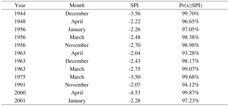
As can be noted from Table 3 the most extreme dry monthly event occurred during the Month of April 2000. This event has a cumulative probability equal to 99,87%. No extreme dry SPI
value was observed during the 1980’s. The years of 1956 and 1963 present three months with
extreme low SPI values. By considering the analyzed period (1937-2013), one may note that approximately 10% of the 76 years presents at least one extreme dry month that may cause great damage to the crop yield production. In this view, by using equation 3 and the parameters estimated in this study, it is possible to verify that the (average) cumulative probability of occurring at least
one dry month Pr(x≥SPI=-2) during a given year in the location of Ribeirão Preto is approximately
TABLE 3. Probability of occurrence associated with extreme dry months observed for the weather station of Ribeirão Preto, State of São Paulo-Brazil (1937-2012)
Year Month SPI Pr(x≥SPI)
1944 December -3.56 99.70%
1948 April -2.22 96.65%
1956 January -2.26 97.05%
1956 March -2.48 98.38%
1956 November -2.70 98.98%
1963 April -2.04 93.28%
1963 December -2.43 98.17%
1963 March -2.75 99.07%
1975 March -3.50 99.68%
1991 November -2.07 94.12%
2000 April -4.53 99.87%
2001 January -2.28 97.23%
CONCLUSSION
The peaks-over-threshold approach can be used to assess the probability of occurrence of extreme dry SPI monthly values obtained from the Weather Station of Ribeirão Preto - State of São Paulo, Brazil.
When compared to the Block Maxima, the peaks-over-threshold provides a better characterization of the probability of occurrence of extreme low SPI values that describe a shortage of available water for plant growth. Accordingly, we recommend the use of this latter approach to assess the probability of occurrence of an extreme dry month that can cause great damage to crop yield production.
The uncertainties in the parameters estimates should be taken into account when the probability associated with a severe/extreme dry event is being assessed.
REFERENCES
BACK, Á. J.; UGGIONI, E. Aplicação do modelo de pulsos retangulares de Bartlett-Lewis
modificado para estimativa de eventos extremos de precipitação. Engenharia Agrícola, v. 30, n. 6,
p. 1033-1045, 2010.
BLAIN, G.C. Considerações estatísticas relativas à oito séries de precipitação pluvial da Secretaria
de Agricultura e Abastecimento do Estado de São Paulo, Revista Brasileira de Meteorologia, v.24,
n.1, p.12-23, 2009.
BLAIN, G. C. Standardized Precipitation Index based on Pearson type III distribution, Revista
Brasileira de Meteorologia, São José dos Campos,v. 26, n. 2, p. 167-180, 2011
BLAIN, G. C.; KAYANO, M. T. 118 anos de dados mensais do Índice Padronizado de
Precipitação: série meteorológica de Campinas, Estado de São Paulo, Revista Brasileira de
Meteorologia, São José dos Campos,v. 26, n. 1, p. 137-148, 2011
BLAIN, G. C. Revisiting the probabilistic definition of drought: strengths, limitations and an
BLAIN, G. C. Monthly values of the standardized precipitation index in the State of São Paulo,
Brazil: trends and spectral features under the normality assumption, Bragantia, Campinas,v. 71, n.
1, p. 460-470, 2012b
BLAIN, G., C., CAMARGO, M. B. P. Probabilistic structure of an annual extreme rainfall series of
a coastal area of the State of São Paulo, Brazil. Engenharia. Agrícola, v.32, n.3, p.552-559, 2012
BORDI, I.; FRAEDRICH, K.; PETITTA, M.; SUTERA, A.; Extreme value analysis of wet and dry
periods in Sicily. Theoretical and Applied Climatology, v. 87, n. 1-4, p. 61-71, 2007.
CANNON, A.J. A flexible nonlinear modeling framework for nonstationary generalized extreme
value analysis in hydroclimatology. Hydrological Process, v.24, n. 1 , p. 673-685, 2010.
COLES, S. An introduction to statistical modeling of extreme value, London: Springer, 1st ed, 2001,
208p.
COLES, S., PERICCHI, L. Anticipating catastrophes through extreme value modelling. Journal of
the Royal Statistical Society. v.52, n.4, p. 405-416, 2003
DELGADO, J. M.; APEL, H.; MERZ, B. Flood trends and variability in the Mekong river.
Hydrology and Earth System Sciences, v. 14, n. 1, p. 407-418, 2010.
FURIÓ, D.; MENEU, V. Analysis of extreme temperatures for four sites across Peninsular Spain,
Theoretical Applied Climatology, v.24, n. 1, 2010.
GUTTMAN, G. B. Accepting the “Standardized Precipitation Index”: a calculation algorithm
index. Journal of the American Water Resources, v. 35, n. 2, p. 311-322, 1999.
HAYES, M. J.; SVOBODA, M. D.;WALL, N.; WIDHALM, M. The Lincoln Declaration on
Drought Indices - Universal meteorological drought index recommended. Bulletin of the American
Meteorological Society, v. 92, n. 4, p. 485-488, 2011.
HADDAD, K., RAHMAN, A. Selection of the best fit flood frequency distributionand parameter
estimation procedure: a case study for Tasmania in Australia. Stochastic Environmental Research
and Risk Assessment, v. 25, n. 3, p. 415-428, 2011.
KATZ, R. W. Statistics of extremes in climate change. Climatic Change, v. 100, n.1, p. 71–76,
2010.
MADSEN, H., RASMUSSEN, P. F., ROSBJERG, D. Comparison of annual maximum series and partial duration series methods for modeling extreme hydrologic events: 1. At-site modeling.
WaterResources Research, v. 33, n.4, p. 747–757, 1997
SANTOS, J. F., PULIDO-CALVO, I., PORTELA, M. M. Spatial and temporal variability of
droughts in Portugal. Water Resources Research, v. 46, n.1, p.1-13, 2010
SANTOS, J. F., PORTELA, M. M.. PULIDO-CALVO, I. Regional Frequency Analysis of
Droughts in Portugal. Water Resources Manage, v. 25, n.1, p.3537-3558, 2011
SHIN, H.; JUNG, Y.; JEONG, C. Assessment of modified Anderson–Darling test statistics for the
generalized extreme value and generalized logistic distributions Stochastic Environmental Research
Risk Assessment, v. 26, n. 1, p. 105-114, 2012.
SUGAHARA, S., DA ROCHA, R. P., SILVEIRA, R. Non-stationary frequency analysis of extreme daily rainfall in Sao Paulo, Brazil. International Journal of Climatology, v. 29, n. 9, p. 1339–1349,
2009.
VLČEK, O., HUTH R. Is daily precipitation Gamma-distributed? Adverse effects of an incorrect
application of the Kolmogorov-Smirnov test. Atmospheric Research v. 93, n.4, p. 759-766, 2009
WILKS, D.S. Statistical methods in the atmospheric sciences, San Diego: Academic Press, 3rd ed,