A Stochastic Dynamic Programming Model for
Valuing a Eucalyptus Investment
M. Ricardo Cunha1 and Dalila B. M. M. Fontes2
1
Universidade Católica Portuguesa and Lancaster University Faculdade de Economia e Gestão
R. Diogo Botelho, 1327 4169-005 Porto, Portugal. [email protected]
2
Faculdade de Economia da Universidade do Porto and LIAAD – INESC Porto L. A. Rua Dr. Roberto Frias, 4200-464 Porto, Portugal.
Abstract
This work proposes an exercise-dependent real options model for the valuation and optimal harvest timing of a forestry investment in eucalyptus. Investment in eucalyptus is complex, as trees allow for two cuts without re-plantation, and have a specific time and growth window in which they are suitable for industrial proc-essing into paper pulp. Thus, path dependency in the cutting options is observed, since the moment of exercise of the first option determines the time interval in which the second option may be exercised. Therefore, the value of the second op-tion depends on the history of the state variables rather than on its final value. In addition, the options to abandon the project, or convert land to another use, are also considered. The option value is estimated by solving a stochastic dynamic programming model. Results are reported for a case study in the Portuguese euca-lyptus forest which show that price uncertainty postpones the optimal cutting deci-sions. Moreover, optimal harvesting policies deviate from present practice of for-est managers and allow for considerable gains.
Key words. Real Options, Dynamic Programming, Forestry Investments,
Bi-nomial Lattice.
1. Introduction
Traditionally, forestry investment decisions were analyzed by using Discounted Cash Flow (DCF) techniques. Given their inability to account for flexibility, these approaches tend to systematically undervalue investments. DCF techniques are based on the assumption that future cash flows follow a constant pattern and can be accurately predicted. The project uncertainty, which may arise from the uncer-tainty about costs, selling prices, weather and legal conditions, to name but a few,
and the flexibility, given to managers to react to changing conditions, are dealt with only superficially [20]. Another disadvantage of DCF is that it is linear and static in nature. It also assumes the project to be either irreversible or if reversible only decisions of now-or-never are allowed [10]. In particular, net Present Value (NPV) takes the project risk into consideration by discounting expected cash flows to the present moment. This discount considers risk either by using certainty-equivalent cash flows [24], or by discounting cash flows using a risk adjusted dis-count rate that can be obtained either through the use of the capital asset pricing model [25] or from a comparison with the market return rates of “similar or risk equivalent” investments. This last approach is the most generalized among practi-tioners. Using this decision process, all projects with positive NPV are undertaken, as they provide an “effective” growth in the wealth of the investor (or market value of the firm). Forest investors, namely paper pulp production companies, use the NPV to decide whether to enter or not a specific investment project. The NPV technique, by not accounting for managerial flexibility, provides an underestimate of the project value, relative to real options. Therefore, when there is an option element in an investment, traditional DCF techniques may result in wrong project valuation and hence inadequate decisions, see e.g., [21] and [10].
Although the writings of Aristotle in Ancient Greece already mention the exis-tence of such features in business and investment, only in the seventies applica-tions to natural resources management have been known [14, 3]. Many other re-searchers have treated the question of replacing a forest stand with the same or other land use, the value of both being stochastic, e.g. [30], [23] and [1].
In a real options model of forestry, and particularly in eucalyptus, the basis starting point is that the owner of the forest holds a call option1, i.e., an option to acquire timber at an exercise price given by the cost of cutting the timber. This forestry option is similar to what in the finance literature is called an American op-tion, since it can be exercised at any moment within the time interval during which the wood is suitable for pulp and paper production. Traditionally, studies address-ing real options in a forest context have applied a saddress-ingle option approach [18]. Such studies are however not suitable for the valuation of multiple harvesting for-estry investments, as investments in eucalyptus. Our study goes consequently be-yond previous studies by considering two cutting options, with potential exten-sions. Therefore, we have to decide when to harvest having in mind that a second harvest is possible and also that the latter must occur within a time window de-pendent on when the previous harvest has taken place. Unlike the single rotation problem, the multirotation case represents a path dependent option, which is far more complex, see [28]. In this case, the option value depends also on the history
1
An option is the right, but not the obligation, to take some action in the future under specified terms. A call option gives the holder the right to buy a stock at a specified future date (maturity) by a specified price (exercise or strike price). This option will be exercised (used) if the stock price on that date exceeds the exercise price.
of the underlying state variables rather than only on their final value. Therefore, the project value today depends on the quantity of timber, which in turn depends on the timing of the previous harvest. In addition, we also consider the options to convert land usage and abandon project.
Results are provided for a case study involving the investment in eucalyptus pulp production for the Portuguese paper industry, one of the most developed in the world. In this case study, two scenarios are considered: one where eucalyptus wood is sold to pulp and paper companies (base problem) and another where ver-tical integration is considered, i.e., wood is processed into white paper pulpwood, which is then sold (extended problem).
After determining the maximum expected value of the investment, we retrieve the policy associated with such a value. Then, in order to test the quality of the cutting strategy and its robustness, we apply the strategies obtained to randomly generated data and compare the values obtained with the current practice of forest managers.
2. Literature Review
In 1973 for the first time, Black & Scholes [5] and Merton [19] provided a closed form solution for the equilibrium price of a call option, leading to a new paradigm in asset valuation. The model they developed gave origin to numerous papers and empirical research in contingent claims analysis, and to applications to many types of contingent claims. Among these, valuation models for real invest-ments have appeared, giving birth to the real options theory of investment deci-sions.
To this date, not many studies have addressed forestry investments using a real options perspective and, as far as the authors are aware of, no previous work has been developed in what concerns investment in eucalyptus forests. Morck et al. [20] developed a contingent claims analysis of a long-term investment in renew-able resource investments. They have extended the general model of valuation of natural resources developed for a gold mining application [6]. Their model values a forestry lease and determines the optimal timing to harvest the timber. The value of the lease is considered to be the value of an option to cut down the trees at the best possible timing. In their model the timber selling price and the inventory of timber are stochastic processes that follow geometric brownian motions. Zinkhan [30] proposes a Black-Scholes type of approach for the valuation of the land use conversion option when valuing timberlands. The conversion option represents the ability of the timberland owner to convert the land use from timber to some other alternative use. Thomson [26] develops this model further in an attempt to in-crease its consistency and simplicity. In both works it is assumed that the land owner holds a European option rather than an American one. Bailey [4] proposes a model to value an agricultural producer considering optimal shutting and reopen-ing and volatile output and demand. However, in what concerns forestry, the model is built only for productive trees with periodical (e.g., annual) harvest. This
characteristic of the model makes it useless for our purpose of valuation of for-estry investment in eucalyptus for paper pulp production, where after two cuts the asset is “worthless” for the paper industry. Abildtrup & Strange [1] analyze the decision to convert a natural or semi-natural forest into Christmas tree production, when groundwater contamination is irreversible and future returns on non-contaminated groundwater resources and Christmas tree production are uncertain. These authors concluded that conventional expected NPV analysis may not lead to an optimal decision rule, and show that the option to postpone conversion and ac-quire new information should be included. Yin [29] discusses harvest timing, land acquisition, and entry decisions combining forest level analysis and options valua-tion approach. Other authors have studied the impact of assuming that stochastic prices follow a mean reverting process rather than geometric brownian motion, see e.g., [16] and [13].
Most of the studies addressing real options in the forest investment context have applied a single option approach. However, exceptions can be found in the literature. Some authors consider additional problem features, while others con-sider more than a single option. For example, Malchow-Mollera et al. [18] include temporal and spatial arrangement of harvests. These authors consider that con-straints upon harvesting options on adjacent forest stands are imposed and exam-ine the optimal harvest rules under adjacency restrictions and uncertainty. They conclude that the costs of adjacency constraints tend to increase with uncertainty and that the optimal harvesting strategies become rather complex due to the inter-action of the involved stochastic variables. Duku-Kaakyire & Nanang [11] devel-oped a forestry investment analysis where four management options are consid-ered: delay of reforestation, capacity expansion, investment abandonment, and a compound option obtained considering simultaneously all three previous options. The models developed are valued on a standard binomial lattice. The authors solve an example with which they show that DCF techniques value the investment as unprofitable, consequently rejecting it. Real options, however, show the invest-ment to be highly valuable. Insley & Rollins [16] model the harvesting problem assuming infinite rotations as a linear complementarity problem that was solved numerically. The accuracy of the solution, obviously, depends on the grid used. Given the computational experiments performed the authors were able to conclude that the value of the harvesting option can be very sensitive to the number of dis-crete levels of the stochastic variable.
In this work, the main objective is to develop a methodology that allows for the valuation of the investment in eucalyptus forest and also to find an optimal har-vesting policy, considering the managerial flexibility inherent to the process. Al-though a similar problem to that of Insley & Rollins [16] is addressed, their meth-odology cannot be applied to eucalyptus forestry investments, since they consider an infinite time horizon framework. Furthermore, this study goes beyond the usual valuation approach since the harvesting policies found are tested by being re-applied to specific data, both real and random.
3. Problem Description
The investment decision under consideration includes three main options: the option to cut down the trees; the option to postpone or defer the trees harvesting until the price or quantity is favorable; and the option to convert the land to an-other use or to abandon the project. We model and solve the problem by consider-ing a compound option obtained by considerconsider-ing all the aforementioned options simultaneously. It should be noticed that the decision of when to harvest the trees is associated with both harvesting options (cut and postponement). Furthermore, these decisions and thus options, must be taken twice since the eucalyptus globu-lous plantations allows for two rotations without replantation.
Many variables guide the profitability of the investment in eucalyptus. Nature, for example, has a major role in the growth of trees. Therefore, the inventory of timber is a very important decision factor. In this work timber inventory is consid-ered to follow a deterministic process with a known growth pattern depending on the region under consideration, the time since last cut (or plantation), and rotation. Also, an obviously very important factor for the decision making is the paper pulpwood selling price, since it determines the main positive cash flow. This price is stochastic and it is assumed to follow a geometric brownian motion. This is fur-ther discussed in Section 1.
The investment decisions
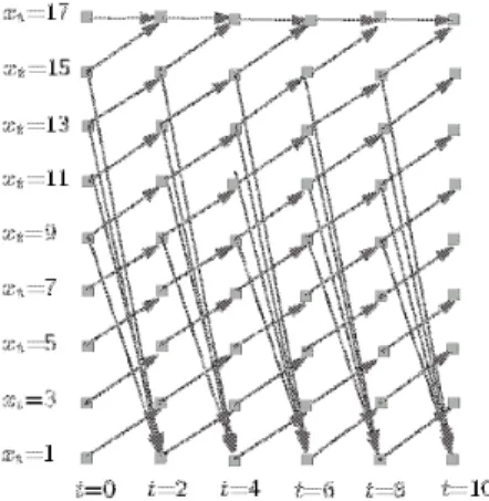
During the investment process in forestry, and particularly in eucalyptus, when the tree is mature, the landowner possesses the option to cut down the trees and receive the resulting cash flow. On the other hand, such a decision may be post-poned if price and/or wood inventory conditions are not favorable. This option is similar to a financial option on a stock, where the underlying asset is the amount of wood in the land and the strike price is the cost of cutting the trees and logging the wood. However, as previously explained, the investment process in eucalyptus is normally composed of two rotations (production cycles). The trees planted at the beginning of the process are suitable for two cuts - after the first cut trees re-grow, permitting a second cut without replantation. Regarding the timing of cut, the characteristics of the wood that could be extracted from trees which are up to 7 years old do not fit the requirements of the industrial producers of pulpwood. The same happens after 16 years of growth, when the diameter of the trees becomes too large for its industrial processing and the fiber in the wood is not of the re-quired standards. Thus, the window time frame is 9 years, for both rotations. However, as the time of exercise of the first option determines the time window during which the second option may be exercised, its temporal location depends on the timing of the first cut. Furthermore, the total expected payoff to be received is given by the sum of the first and second harvesting expected cash flows. Given the path dependency observed, the cash flow received from the second harvesting depends upon the timing of the first harvesting. This dependency leads to a
multi-plicity of possible paths and strategies, as can be seen in the state transition dia-gram given in Figure 1. In this diadia-gram we have represented the time
t
and the elapsed time since last cut or plantationx
t, with a 2-years step interval.Figure 1: State transition diagram: 2-years step interval.
The cash flow to be received from harvesting the trees depends on the cutting period - since the quantity of wood, although known, evolves through time - and on wood market price and future value expectations. Moreover, the decision of cutting the trees in the first rotation must consider not only the immediate cash flow, but also the expectation of the cash flow from the second rotation.
In our analysis, the eucalyptus forest investor is assumed to hold the land. Therefore, at any moment in time the investor holds the option to abandon the pro-ject and put it aside, or receive an estimated value from converting the land into an alternative use. Activities like tourism and hunting have increased the demand for forest land and hence, its value. This alternative value (or capacity to abandon without a loss greater than the initial land acquisition investment) must then be considered in the valuation of eucalyptus forest investment.
4. Methodology
The approach developed consists of a dynamic programming model which is evaluated on a discrete-valued lattice. The uncertainty of the underlying risky as-set, wood or paper pulp selling price, is modeled through the use of a standard bi-nomial lattice. This approach is described in the following section. To develop the dynamic programming model, we first must define and explain the decision vari-ables as well as the state varivari-ables. The decision varivari-ables are associated with the possible strategic decisions that investors and managers may undertake during the investment process, while the state variables are related to time, see Section 2. In Section 3 we present the dynamic programming model and explain how to solve it
through backward induction. The optimal value of the investment project and the corresponding optimal harvesting strategy are given by the solutions to the pro-posed model.
4.1. The binomial lattice
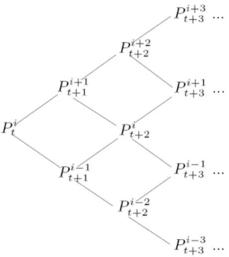
The analysis performed in this work makes use of the multiplicative binomial model of Cox, Ross & Rubinstein [8], the standard tool for option-pricing in dis-crete time. In this approach, the stochastic variable (the selling price in our case) is assumed to be governed by a geometric diffusion, which implies that at each pe-riod there is only one constant growth/decay rate. If this is assumed, a natural way of obtaining a valued-lattice for the stochastic variable is to discretize it through a standard binomial lattice, see Figure 2.
Figure 2. A lattice discretizing selling price.
A node of price value
P
tican lead to two nodes with their values being given byP
ti++11=
uP
ti andP
t+i−11=
dP
ti with probabilityp
andq
=
1
−
p
, respectively. The probability of reaching each of these nodes is the usual equivalent martingale measure used in the binomial option pricing model of Cox et al. (1979):d
u
d
r
p
f−
−
+
=
(
1
)
andq
=
1
−
p
(1) wherer
f is the risk free interest rate over the interval∆
t
,u
=
exp(
σ
∆
t
)
,)
exp(
t
as
∆
t
→
0
the parameters of the multiplicative binomial process converge to the geometric brownian motion.The advantages of this approach are that (i) it can be used to price options other than European, like American and path dependent options; (ii) it does not depend on the investor subject probabilities of an upward/downward price movement, since it uses risk neutral probabilities; and (iii) it is intuitive and simple to under-stand and implement.
The binomial model breaks down the investment horizon into
n
time intervals or steps. The lattice is then developed in a forward movement by finding the value of selling prices. At each step the price moves up or down by an amount obtained from its volatility, which is assumed to be constant and known, and the time step length. Thus, the lattice provides a representation of possible selling prices throughout the whole project life.4.2. Decision and state variables
The selling price variable
P
ti is modeled as a stochastic variable, which fol-lows a binomial process, as in the previous section.In terms of decisions, as previously described, we consider basically three pos-sibilities: to cut the trees, delay trees cutting, and abandon project or convert land to another usage. Hence, we define a decision variable
D
ti that may assume three values according to the decision taken at timet
and state (price index expecta-tion)i
.
use,
another
to
converted
land
or the
abandoned
is
project
the
if
,
3
,
maintained
investment
the
and
postponed
is
cutting
if
,
2
cut,
are
trees
if
,
1
The inventory of wood is considered to be a deterministic process, following a known growth pattern according to the considered region, the time since last cut (or plantation), and the rotation. The evolution of the time since the first cut (or plantation)
x
tis modeled as:
=
+
=
=
+,
2
if
1
,
1
if
2
1 t t i t tD
x
D
x
and initialized as
x
1=
1
. In the second rotationx
t+1 is initialized as 2, rather than 1, since the trees are already there and thus, do not need to be planted. If the decision is to abandon the project or convert land to another use then the project ends.Regarding the inventory of wood, we need two variables to represent it. One concerning the inventory of wood that is good for paper pulp production and an-other for the wood that does not meet paper pulp industrial requirements. Recall that, as explained before, the wood obtained from trees having up to 7 years of growth, as well as from trees with more than 16 years of growth, does not meet paper pulp industrial requirements. Let
tc
min=
8
andtc
max=
16
be, respec-tively, the minimum and maximum time from plantation (or first cut) for the trees to be suitable for paper production. LetSQ
( )
x
t,
i
andCQ
( )
x
t,
i
be the inven-tory of wood that can be sold to paper pulp production and the inveninven-tory of wood that is extracted from cutting the trees, respectively. On one hand, if tree cutting occurs within 8 to 16 years of growth, then these two figures, obviously, have the same value. On the other hand, if trees are cut before reaching 8 years of growth or after 16 years of growth, thenSQ
is zero2 whileCQ
is positive.( )
( )
( )
( )
( )
( )
<
=
=
<
=
>
<
=
,
if
,
,
if
,
,
,
if
,
,
if
,
,
or
if
,
0
,
2 1 2 1 max mint
x
x
Q
t
x
x
Q
t
x
CQ
t
x
x
Q
t
x
x
Q
tc
x
tc
x
t
x
SQ
t t t t t t t t t t t twhere
Q
1( )
x
t andQ
2( )
x
t are the quantities of wood extracted from cutting the trees which have been growing forx
t years at rotation 1 and rotation 2, re-spectively.4.3. Dynamic programming model
In each period, the forest investor must decide whether the forestry investment is going to be kept or not. Since both for project abandonment and land use con-version options only a lump sum is received, no subdivision is considered regard-ing these options. However, for the former case, the forest investor still has to make a decision regarding the timing of tree harvesting. The investor will choose either to harvest at the current period or to leave the trees there for the next period, whichever yields better expected cash flows.
Harvesting the trees yields the owner revenue from selling the wood but also involves costs
K
incurred with cutting, peeling, and transporting the wood. There-fore, at periodt
, given the elapsed time since last cut or plantationx
t and the
2
Any other value, that could be obtained for the wood, can be used in our model.
price expectation index
i
, the net revenueπ
obtained if the cutting option is ex-ercised is given by(
x
i
t
)
P
iSQ
( )
x
tt
K
CQ
( )
x
tt
t t,
,
=
×
,
−
×
,
π
(2)As described before, in order to allow for earlier exercise, the valuation proce-dure begins at the last stage and works backwards to the initial moment. At the fi-nal lattice nodes, i.e., at the end of the project life
t
=
T
,
all possible selling price values and elapsed time since last cut values are computed. For each of these ter-minal nodes the project value is then given by the largest of (i) the final revenue plus residual value if a harvesting decision is still possible and exercised or (ii) the residual value. Here, by residual valueR
we mean the maximum between aban-doned land value and land conversion value. The land conversion value is as-sumed to have no real appreciation or depreciation. Evidence shows that agricul-tural and forest land values have been stationary. However, in the empirical sections we perform some model sensitivity analysis to the value ofR
. It should be noticed that, after second harvest or at the end of the period of analysis if no second harvest takes place the project value is given by the residual valueR
. Fur-thermore, this value is the same both for the base and the extended problems, which is in accordance with the fact that no additional investment costs have been considered for latter problem.(
)
(
)
+
=
R
R
T
i
x
T
i
x
V
T T,
,
max
,
,
π
(3)The project value at each intermediate lattice node is computed by performing a backward induction process. The project value at intermediate steps is used to compute the project value at previous steps by using risk neutral probabilities. The decision made at any period (and state variable) has implications not only on the cash flow of the current period but also on the expected cash flow of future peri-ods. Therefore, the optimal project value is obtained by maximizing the sum of the current period’s net revenue with the optimal continuation value considering all possible decisions. The optimal project value at period
t
, given the elapsed time since last cut or plantationx
t and the price expectation indexi
,
is then given by(
)
(
)
(
)
(
)
(
)
(
)
= = + + − − + + + = + + − − + + + + = + + + + , 3 if , 2 if r 1 1 , 1 , ) 1 ( 1 , 1 , , 1 if r 1 1 , 1 , ) 1 ( 1 , 1 , , , max , , f 1 1 f 1 1 t t t t t t t t D t D R D t i x V p t i x pV D t i x V p t i x pV t i x t i x V i t π (4)where
π
(
x
t,
i
,
t
)
is the net revenue from the selling of the wood,r
f is the real risk free interest rate,p
is the risk neutral probability of an upward movement inthe binomial price, and
R
is the largest of the abandonment value or conversion to another use value.The estimated project net value is then given by
V
(
1
,
1
,
1
)
(
1
+
r
f)
minus theinitial investment3. Furthermore, the solution to this model also provides an opti-mal decision strategy for the forest manager.
In the following section the dynamic programming model given by equations (3) and (4) is empirically tested through the application to a case study of invest-ment in eucalyptus for the paper pulp industry, in Portugal.
5. Case study
In this section, we start by giving a brief characterization of the Portuguese for-est sector. Secondly, we describe the case study to which our model is to be ap-plied, and end by presenting the results obtained.
5.1 Brief characterization of the Portuguese forest
sec-tor
Portugal, due to its natural characteristics, possesses unique natural and eco-logical conditions for forestry production, which only recently has started to be methodologically and professionally managed. This fact is particularly true for high productivity forest species such as the eucalyptus globulous for the paper in-dustry.
According to forest inventories (DGRF – Database 2001), forest and wooded land represent 37.7% of the Portuguese continental regions. Nowadays, the main species existent in Portuguese forests are pinus pinaster (29.1%), cork oak (21.3%), and eucalyptus (20.1%), the latter being mainly represented by the euca-lyptus globulous species.
The eucalyptus globulous, the main sub-species in our country and the one that possesses the best characteristics for paper production, is a fast growing tree. Originally biologically adapted to the poor soils of the Australian continent, in southern Europe, and Portugal in particular, this species grows very rapidly. Nor-mally, the eucalyptus are cut with an age of 12 years and used to produce pulp-wood, providing cellulose fibers that have remarkable qualities for the production of high quality paper. In what concerns ownership, the pulp industry manages
3
The initial investment is considered to be given by the land acquisition costs, the plantation costs, and the cost of a maintenance contract for the full length of the project. However, this contract does not include cutting, peeling, and transpor-tation of the harvested wood, which account for the exercise price of the cutting option.
proximately 30% of the eucalyptus area in Portugal. The increase in the paper and pulpwood production translated into an increase in real terms of about 50% of the gross value added of the forestry sector, which reveals a much faster growth than the one observed for the rest of the Portuguese economy [7].
Forest and forest related industries are a key sector in the Portuguese economy, generating wealth and employment. The modernization of this sector can be a source of competitive advantage for the country, given the favorable ecological and natural conditions. Due to the development of the paper production industry and the natural characteristics of the species, eucalyptus globulous has shown to be a key player in the sector, with a huge wave of investment in the species in the last decades.
5.2. Data and parameters
The initial investment: plantation and maintenance costs
We assume that the investor contracts all expected operations to a specialized firm at the start of the investment and pays the contract in advance. The operations and their present value costs add up to 3212 euros per hectare, from which 1712 euros correspond to the plantation and the 2 rotations maintenance contract (which can last from 15 to 31 years, with 23 years expected duration), and 1500 euros correspond to the acquisition cost of 1 hectare of land. The details of how these values were obtained are given in Appendix A. Recall that, in this study two sce-narios are considered. The base problem considers that the eucalyptus forest is owned by a forest investor, and that its wood is sold to pulp and paper companies. The extended problem considers that the eucalyptus forest is owned by the paper industry and that the wood is processed into white pulp, which is then sold. The two problems are included in order to distinguish outputs for different types of agents. Hence, the pulpwood productive capacity is considered to be present and its investment is disregarded and treated as a sunk cost, not relevant for undergo-ing investment projects.
Wood and white paper pulpwood prices
The price of wood in the base problem and the price of white paper pulpwood in the extended problem are assumed to follow a binomial stochastic process, as previously explained. We use 2002 prices: 45 euros per cubic meter of peeled eucalyptus wood; and 500 euros per cubic meter of white paper pulp [2]. The prices volatility was extracted from the time series of prices [12,7], considering constant prices of 2002 and using the consumer price index as deflator [15]. The extracted volatility corresponds to the volatility of returns of the three-years mov-ing average of prices. This average was calculated in order to smooth the price se-ries, as jumps in prices were periodical (3 year intervals between jumps). The
price volatility measured by the standard deviation has been computed to be 0.0717 for wood and 0.1069 for white pulpwood.
Wood and white paper pulpwood quantities
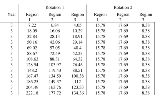
In order to compute the quantities of available wood per ha of eucalyptus forest we have used the inventory model Globulus by Tomé, Ribeiro & Soares [27]. We have considered wood quantities for the three main Portuguese regions in what concerns eucalyptus investment: north central coast (region 1), central coast (re-gion 2), and river Tejo valley (re(re-gion 3). For each re(re-gion and rotation we consider different tree growth patterns. The average growth curve for the amount of wood in a hectare of eucalyptus forest land in each of the regions can be observed in Appendix B. In the extended problem, which uses pulpwood valuation, it has been considered that about 3.07 cubic meters of wood are required to produce 1 ton of white pulp, which corresponds to approximately 1.1 cubic meters of white pulp [27].
The exercise price for the cutting option
K
The exercise price of the cutting option is given by the costs incurred in cutting the trees, peeling the wood, and transporting it to the factory. Considering constant prices of 2002, the total cost is estimated to be 22.5 euros per cubic meter of wood [2]. When considering the extended problem, which takes into account transfor-mation into white pulp, the cost of this transfortransfor-mation must also be taken into con-sideration. The industrial processing cost is approximately 320 euros per ton of white pulpwood4 (200 euros of variable costs and 120 euros of fixed costs). The cost of cutting, peeling and transporting the wood necessary for a ton of white pa-per pulp is 69.14 euros. Therefore, a ton of white papa-per pulp costs 389.14 euros to transform. As 1 ton of white paper pulp corresponds to 1.1 cubic meters, the cost of processing 1 cubic meter of white paper pulp is then 353.76 euros [22].
The risk free interest rate
r
fAs we are working with real prices from the year 2002, we have considered a real risk free interest rate of 3%. This value was approximated through the obser-vation of the Euro yield curve (average nominal risk free interest rate of 5% for long term investments such as the eucalyptus) and the 2% expected inflation target in the Euro area (Eurostat).
4
This value was obtained through the analysis of the operating costs of the pa-per pulpwood companies and their installed capacity, and also through inquiries to experts.
The abandonment and Conversion to another land use value
R
In each time step, the investor possesses the option to abandon the investment project, putting the land aside and/or receiving the market price for agricultural and forest land.
In other situations, the investor may convert the land use into other activities, e.g., tourism, hunting, or real estate development. In this work, we consider both situations. We assume that demand may exist for the land as it is, or for the land to be converted to another use. Several possible values for the conversion value
R
are considered, from the situation where no value is given to the land due to lack of demand, to situations of high conversion values that may arise, for example, due to real estate speculation.
6. Results
In this section, we specify the computational experiments conducted as well as the results obtained. All experiments have been performed using three regions in continental Portugal: 1 – north central coast, 2– central coast, and 3 – river Tejo valley, which present different productivity, as shown in Appendix B.
The results are divided into two sections, one regarding the dynamic program-ming model discussed in the previous section and another regarding the applica-tion of the harvesting strategies obtained to randomly generated data sets. In the first section, we report on the results obtained by applying the aforementioned dy-namic programming model to the base and extended problems. In the second sec-tion, we present results regarding the implementation of the optimal strategies provided by the dynamic programming model to both the base and the extended problem. In order to do so, we randomly generate sets of price data, to which we apply these optimal strategies. The application of these strategies to the randomly generated data only considers the fact that price movements are upwards or downwards, disregarding the magnitude of the movement.
A – Results for the base and extended problems
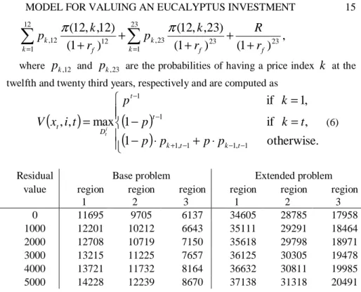
To start with, and in order to have a standard project value, we compute the value of the project considering that cuts are performed at years 12 and 23 respec-tively, the industry common practice. The price values used are the expected value of the price at years 12 and 23. Several possible values are considered for the land residual value. This valuation is in nature a net present value approach. The cut timing strategy considered has been observed to be the most common among eucalyptus forest managers.
The results, reported in Table 1, are computed, for the three above mentioned regions, as
,
)
1
(
)
1
(
)
23
,
,
12
(
)
1
(
)
12
,
,
12
(
23 23 1 23 23 , 12 1 12 12 , f k f k k f kr
R
r
k
p
r
k
p
+
+
+
+
+
∑
∑
= =π
π
(5)where
p
k,12 andp
k,23 are the probabilities of having a price indexk
at the twelfth and twenty third years, respectively and are computed as(
)
(
)
(
)
⋅
+
⋅
−
=
−
=
=
− − − + − −otherwise.
1
,
if
1
,
1
if
max
,
,
1 , 1 1 , 1 1 1 t k t k t t D tp
p
p
p
t
k
p
k
p
t
i
x
V
i t (6)Residual Base problem Extended problem value region 1 region 2 region 3 region 1 region 2 region 3 0 11695 9705 6137 34605 28785 17958 1000 12201 10212 6643 35111 29291 18464 2000 12708 10719 7150 35618 29798 18971 3000 13215 11225 7657 36125 30305 19478 4000 13721 11732 8164 36632 30811 19985 5000 14228 12239 8670 37138 31318 20491 Table 1. Common practice project value, for varying residual values.
Regarding the values obtained by our model, and in order to show that the postpone and abandonment/conversion options interact, we value the project con-sidering (i) that only the harvesting and postponement options exist and (ii) that all options exist. Furthermore, the project is valued considering several land residual values
R
.For the results presented in Table 2, where only the harvesting and postpone-ment options exist, the residual value
R
is only recovered at the end of the pro-ject. This happens, at timeT
or either whenever the two possible cuts have al-ready been performed or no further cutting is allowed.Residual Base problem Extended problem value region 1 region 2 region 3 region 1 region 2 region 3 0 15959 13084 8186 51295 42116 26030 1000 16371 13496 8599 52114 42935 26849 2000 16784 13909 9012 52934 43755 27667 3000 17196 14322 9426 53753 44574 28488 4000 17609 14735 9842 54573 45396 29308 5000 18022 15149 10261 55393 46219 30128 Table 2. Real options project value, for varying residual values.
When considering all options the residual/conversion land value is obtained in the same conditions as above or whenever it is optimal to give up further harvest-ing. In the experiments performed, we have considered that the value to be recov-ered is the residual value
R
, since a better comparison with the results obtained when considering only the harvesting and postponement options, is possible. It should be noticed that, by doing so we are considering an abandonment option. In here, we only report one set of results, since the results obtained for cases (i) and (ii) were the same. Differences in the project value when considering all options began to appear only when there is an abnormal demand for the land, which ap-preciates its value to levels several times the considered acquisition value.The differences in valuation between the standard NPV approach, typically used by the industry, and the options approaches here presented are clear. The real options approach, due to the consideration of the flexibility in the management of the forest, allows for much higher values. It provides a revenue increase that can go up to 36.46% for the base problem and up to 49.15% for the extended problem. It should be noticed that the increase decreases with the residual value, since the higher the residual value the smaller is the impact of the harvesting strategy on project value.
Another main conclusion that can be drawn is that the different sources of flexibility clearly interact. However, the difference in valuation considering the presence of all options and only the main cutting options is only relevant if sidering very high residual values. This does not come as a surprise, since we con-sider that the residual value is a fixed value in time. Given that we are discounting future cash flows, then the residual present value decreases with project time hori-zon. Furthermore, we are not considering a real and specific land conversion value, which can often be much larger than the abandonment value.
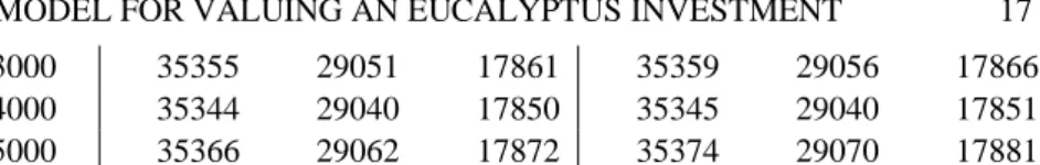
Before comparing the results obtained for the base problem and the extended problem, let us recall what these problems represent. The base problem considers the situation where the forest is considered to be privately owned, and the eucalyp-tus wood is sold to paper industry companies. The extended problem, however, considers vertical integration of wood and paper production. The value added by the ownership of forest land being in the hands of the pulp industries (or the value added through vertical integration) can be estimated through the difference be-tween the project values for the base and the extended problems, as given in Table 3. Recall that, for the extended problem, no additional investment costs are being considered, thus to the value added through vertical integration we still have to deduct the aforementioned investment costs.
Residual Harvest and postpone options All options value region 1 region 2 region 3 region 1 region 2 region 3 0 35339 29035 17845 35339 29035 17844 1000 35344 29040 17850 35345 29040 17851 2000 35344 29040 17850 35345 29040 17851
3000 35355 29051 17861 35359 29056 17866 4000 35344 29040 17850 35345 29040 17851 5000 35366 29062 17872 35374 29070 17881 Table 3. Project value differences between base and extended problems, for varying residual values.
As it can be observed, the difference in project value is small and basically constant across the different residual values considered, that is, it almost does not depend on the residual value. Nevertheless, the value added through vertical inte-gration seems to be extremely high, and justifies the observed direct and indirect investment of paper industry companies, out of their core business of paper pulp production, into producing the inputs themselves. Furthermore, as expected, the larger differences are observed for the most productive regions. However, care should be taken in drawing conclusions, since non-neglectful investments may be required for the vertical integration to take place. As these costs have not been ac-counted for in the results, the benefits of vertical integration are overestimated. This overestimation is however not as large as it might seem, as the residual value - the value of the firm at the end of the project - is the same for both problems.
C – Applying the optimal strategies
In order to evaluate the quality of the optimal strategy produced by our dy-namic programming model, we apply the strategy provided by the model when considering all options, to randomly generated price data sets. The project value obtained in this way is then compared to the one that would be obtained by the common practice of harvesting after 12 years of growth. Five data sets have been randomly generated according to the characteristics given in Table 4. The charac-teristics reported are relative to the price values used in the case study.
Data Price values
Set minimum maximum average
1 80% 100% 80%
2 100% 100% 90%
3 100% 100% 100%
4 100% 100% 110%
5 100% 120% 120%
Table 4. Characteristics of the randomly generated data sets.
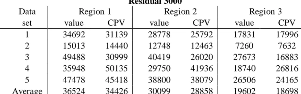
We report the project value obtained by applying the optimal strategies devised both for the base and the extended problems. These results are provided for the 5 randomly generated data set types. We also report on the common practice project value (CPV) obtained by performing the harvest at years 12 and 23, see tables 5 to 8 for different residual values.
Residual 0
set value CPV value CPV value CPV 1 33492 29619 27578 24271 16631 16476 2 13813 12920 11548 10943 6060 6112 3 48288 29479 39219 24500 26473 15363 4 34748 48615 28550 40416 17540 25296 5 46278 43898 37600 36559 25306 22645 Average 35324 32906 28899 27338 18402 17178 Table 5. Project value considering a residual of 0 for all regions when decision strategies are ap-plied to specific data sets.
Residual 1000
Data Region 1 Region 2 Region 3 set value CPV value CPV value CPV
1 33892 30126 27978 24778 17031 16983 2 14213 13426 11948 11450 6460 6619 3 48688 29986 39619 25006 26873 15869 4 35148 49121 28950 40922 17940 25803 5 46678 44404 38000 37066 25706 23151 Average 35724 33413 29299 27844 18802 17685 Table 6. Project value considering a residual of 1000 for all regions when decision strategies are applied to specific data sets.
Residual 3000
Data Region 1 Region 2 Region 3 set value CPV value CPV value CPV
1 34692 31139 28778 25792 17831 17996 2 15013 14440 12748 12463 7260 7632 3 49488 30999 40419 26020 27673 16883 4 35948 50135 29750 41936 18740 26816 5 47478 45418 38800 38079 26506 24165 Average 36524 34426 30099 28858 19602 18698 Table 7. Project value considering a residual of 3000 for all regions when decision strategies are applied to specific data sets.
Residual 5000
Data Region 1 Region 2 Region 3 set value CPV value CPV value CPV
1 35492 32153 29578 26805 18631 19009 2 15813 15453 13548 13476 8060 8645 3 50288 32013 41219 27033 28473 17896 4 36748 51148 30550 42949 19540 27830 5 48278 46431 39600 39093 27306 25178 Average 37324 35440 30899 29871 20402 19712
Table 8. Project value considering a residual of 5000 for all regions when decision strategies are applied to specific data sets.
As it can be seen, in the above situations the project has a larger value when computed using the real options approach. Region 1, the north central coast, is the most appropriate area in the country for eucalyptus and thus, the most productive. Results for the other two regions also provide the same conclusions.
It should be noticed that the harvesting decisions typically take place after six-teen years of growth for both rotations. This corresponds to the maximum time growth allowed. Thus, it can be concluded that the cutting option is exercised al-most always at maturity, which allows for the investor to take advantage of the full tree growth. This fact is inconsistent with the common practice of most forest producers. The urge to cash in the value of their eucalyptus wood, due to high risk aversion, typically made at the 12th year seems to be not optimal. A possible ex-planation may be that once the second cut is performed, then the project can be re-peated and given the human life expectancy it may not make sense to wait longer than the minimum required time.
7. Conclusions
In this work, we address the valuation of an investment in eucalyptus forest land for the paper pulp industry by using real options theory. The modeling of the eucalyptus forest investment decisions using real options theory allows for valua-tion results more consistent with the normal positive investment outcomes than the ones obtained using traditional valuation techniques. The interpretation of the two possible tree cuts as two exercise interdependent call options on the wood allows for the introduction of managerial flexibility in the forest management process. The inclusion of the abandonment and conversion to another use options increases the closeness to the real decision process.
The evidence in this paper, through the application of the developed stochastic dynamic programming model to the eucalyptus investments in three Portuguese regions and for randomly generated situations, is consistent with the experts’ warnings of the under-valuation performed by traditional discounted cash flow techniques. A rationale for the trend of vertical integration of paper pulp and wood production is also provided by the value difference between the two problems considered.
It is also shown that typical cutting time decisions by forest owners are not consistent with cash flow maximization. According to our model, cutting should be almost in all situations performed at the end of the time interval when wood is suitable for paper pulp production.
Acknowledgments
The authors would like to thank FCT for the financial support through scholar-ship BD/12610/03 and project POCI/MAT/61842/04.
Appendix A
Initial investment: operation costs and present values
Year Maintenance Operations Operation costs (eu-ros)
2002 Present
value 1 Soil preparation and fertilization
Plantation Infrastructures - Paths 1100 1100 1 Replantation (10-15% of planted trees) 60 60 2 Soil fertilization 62.5 60.6 3 Soil cleaning (Milling cutter) 90 84.8 4 Soil fertilization
Infrastructures cleaning 100 91.5 7 Soil cleaning (Disc harrow)
Infrastructures cleaning 100 83.7 12 Infrastructures cleaning 10 7.2 14 Soil fertilization 55 37.4 15 Road selection 90 59.5 16 Soil fertilization Infrastructures cleaning 100 64.1 19 Soil cleaning (Disc harrow)
Infrastructures cleaning 100 58.7 24 Infrastructures cleaning 10 5
Value of plantation and maintenance contract 1712
Appendix B
Rotation 1 Rotation 2 Year Region 1 Region 2 Region 3 Region 1 Region 2 Region 3 3 7.22 6.84 4.05 15.78 17.69 8.38 3 18.09 16.06 10.29 15.78 17.69 8.38 3 32.84 28.14 18.91 15.78 17.69 8.38 3 50.16 42.06 29.14 15.78 17.69 8.38 3 69.02 57.05 40.4 15.78 17.69 8.38 3 88.67 72.59 52.23 15.78 17.69 8.38 3 108.63 88.31 64.32 15.78 17.69 8.38 3 128.54 103.97 76.46 15.78 17.69 8.38 3 148.2 119.43 88.51 15.78 17.69 8.38 3 167.47 134.59 100.38 15.78 17.69 8.38 3 186.25 149.37 112 15.78 17.69 8.38 3 204.49 163.76 123.33 15.78 17.69 8.38 3 222.18 177.72 134.36 15.78 17.69 8.38Table 10. Quantities of eucalyptus wood, in
m
3 per ha .References
[1] Abildtrup, J. & Strange, N. (1999), ‘The option value of non-contaminated forest watersheds’, Forest Policy and Economics 1, 115–125.
[2] Aliança Florestal (2002), Technical Internal Report: www.alflorestal.pt. [3] Arrow, K. & Fisher, A. C. (1974), ‘Environmental preservation, uncertainty
and irreversibility’, Quarterly Journal of Economics 88, 312–319. [4] Bailey, W. (1991), ‘Valuing agricultural firms: An examination of the
contin-gent claims approach to pricing real assets’, Journal of Economic Dy-namics and Control 15, 771–791.
[5] Black, F. & Scholes, M. (1973), ‘The pricing of options and corporate liabili-ties’, Journal of Political Economy 27, 637–654.
[6] Brennan, M. & Schwartz, E. (1985), ‘Evaluating natural resource investments’, Journal of Business 58, 135–157.
[7] CELPA – (Associação da Indústria Papeleira), www.celpa.pt.
[8] Cox, J., Ross, S. & Rubinstein, M. (1979), ‘Option pricing: a simplified ap-proach’, Journal of Financial Economics 12, 229–263.
[9] DGRF – Database (2001), Inventário Florestal Nacional by Direcção Geral dos Recursos Florestais: www.dgf.min-agricultura.pt.
[10] Dixit, A. & Pindyck, R. S. (1994), Investment under uncertainty, Princeton University Press, Princeton, New Jersey.
[11] Duku-Kaakyire, A. & Nanang, D. M. (2004), ‘Application of real options theory to forestry investment analysis’, Forest Policy and Economics 6, 539–552.
[12] FAO – (Food and Agricultural Organization of the United Nations),
www.fao.org.
[13] Gjolberg, O. & Guttornmsen, A. G. (2002), ‘Real options in the forest: What if prices are mean reverting’, Forest Policy and Economics 4, 13–20. [14] Henry, C. (1974), ‘Option values in the economics of irreplaceable assets’,
Review of Economic Studies 41, 89–104.
[15] INE – Infoline (2001), Instituto Nacional de Estatística: www.ine.pt.
[16] Insley, M. (2002), ‘A real options approach to the valuation of a forestry in-vestment’, Journal of Environmental Economics and Management 44, 471–492.
[17] Insley, M. & Rollins, K. (2005), ‘On solving the multirotational timber har-vesting problem with stochastic prices: a linear complementarity formu-lation’, American Journal of Agricultural Economics 87, 735755. [18] Malchow-Mollera, N., Strangeb, N. & Thorsen, B. J. (2004), ‘Real-options
aspects of adjacency constraints’, Forest Policy and Economics 6, 261– 270.
[19] Merton, R. C. (1973), ‘An intertemporal capital asset pricing model’, Econo-metrica 41, 867–887.
[20] Morck, R., Schwartz, E. & Stangeland, D. (1989), ‘The valuation of forestry resources under stochastic prices and inventories’, Journal of Financial and Quantitative Analysis 24(4), 473–487.
[21] Pindyck, R. S. (1991), ‘Irreversibility, uncertainty, and investment’, Journal of Economic Literature 29(3), 1110–1148.
[22] Portucel Setúbal (2002), Technical Internal Report: www.portucelsoporcel.com.
[23] Reed, W. (1993), ‘The decision to conserve or harvest old-growth forest’, Ecological Economics 8, 45–49.
[24] Robichek, A. A. & Myers, S. (1966), ‘Conceptual problems in the use of risk-adjusted discount rates’, Journal of Finance 21, 727–730.
[25] Sharpe, W. F. (1964), ‘Capital asset prices: A theory of market equilibrium under conditions of risk’, Journal of Finance 19(3), 425–442.
[26] Thomson, T. A. (1992), ‘Option pricing and timberlands land-use conversion option: comment’, Land Economics 68, 462–469.
[27] Tomé, M., Ribeiro, F. & Soares, P. (2001), O modelo glóbulus 2.1, Technical report, Grupo de Inventariação e Modelação de Recursos Naturais, De-partamento de Engenharia Florestal, Instituto Superior de Agronomia, Universidade Técnica de Lisboa.
[28] Wilmott, P. (1998), Derivatives, the Theory and Practice of Financial Engi-neering, Wiley, Chickester.
[29] Yin, R. (2001), ‘Combining forest-level analysis with options valuation ap-proach – a new framework for assessing forestry investment’, Forest Sci-ence 47(4), 475–483.
[30] Zinkhan, F. (1991), ‘Option pricing and timberlands land-use conversion op-tion’, Land Economics 67, 317–325.