Abstract
Extensive research has been applied to discover new techniques and methods to model protein-ligand interactions. In particular, considerable efforts focused on identifying candi-date binding sites, which quite often are active sites that correspond to protein pockets or cavities. Thus, these cavities play an important role in molecular docking. However, there is no established benchmark to assess the accuracy of new cavity detection methods. In prac-tice, each new technique is evaluated using a small set of proteins with known binding sites as ground-truth. However, studies supported by large datasets of known cavities and/or binding sites and statistical classification (i.e., false positives, false negatives, true positives, and true negatives) would yield much stronger and reliable assessments. To this end, we propose CavBench, a generic and extensible benchmark to compare different cavity detec-tion methods relative to diverse ground truth datasets (e.g., PDBsum) using statistical clas-sification methods.
Introduction
Modeling protein-ligand interactions is crucial to drug discovery and design, as well as to understand bio-molecular structures. While extensive efforts have been applied for many years into discovering new methods to model protein-ligand interactions, a comprehensive mecha-nism to compare and assess such methods (and algorithms) is still lacking. This makes it diffi-cult to properly ascertain the contributions of each method in the context of the myriad of approaches developed over the past decades.
In the present work, we are particularly interested in benchmarking protein cavity (or pocket) detection methods against one or more databases of cavities (e.g., PDBsum [1,2]) or even databases of already-known binding sites (e.g., scPDB [3]). Often, these already-known protein binding sites correspond to protein cavities, so they may also work as ground-truth cavities. This explains why detecting pockets/cavities on protein surfaces is an important first step toward identifying protein binding sites for small molecules or ligands [4–6]. Thus, pocket detection plays an important role in protein-ligand docking and structure-based drug design. a1111111111 a1111111111 a1111111111 a1111111111 a1111111111 OPEN ACCESS
Citation: Dias S, Simões T, Fernandes F, Martins AM, Ferreira A, Jorge J, et al. (2019) CavBench: A benchmark for protein cavity detection methods. PLoS ONE 14(10): e0223596.https://doi.org/ 10.1371/journal.pone.0223596
Editor: Manuela Helmer-Citterich, Universita degli Studi di Roma Tor Vergata, ITALY
Received: April 26, 2019 Accepted: September 24, 2019 Published: October 14, 2019
Copyright:© 2019 Dias et al. This is an open access article distributed under the terms of the Creative Commons Attribution License, which permits unrestricted use, distribution, and reproduction in any medium, provided the original author and source are credited.
Data Availability Statement: The software is available athttps://github.com/mosqueteer/ CavBenchand the datasets are available from https://figshare.com/articles/CavBench_datasets/
9917087.
Funding: This research has been partially supported by the Portuguese ResearchCouncil (Fundac¸ão para a Ciência e Tecnologia), under the FCT Projects UID/EEA/50008/2019, UID/CEC/ 50021/2019, PTDC/EEI-SII/6038/2014, the doctoral grant SFRH/BD/99813/2014, and postdoctoral grants SFRH/BPD/97449/2013 and
Many protein cavity detection methods have been proposed in the literature for the last 35 years (see, for example, [4,7–17]). However, only a few times have we seen such methods vali-dated or certified relatively to a ground-truth underlying a database of known cavities or a database of known binding sites. This is largely because the first such databases only made their appearance in the early 2000s, after the debut of DIP (Database of Interacting Proteins) available athttp://dip.doe-mbi.ucla.edu/for protein-protein interactions [18], in particular BIND (Biomolecular Interaction Network Database) athttps://bio.tools/bind[19] and Bin-dingDB (https://www.bindingdb.org/bind/index.jsp) [20,21] for interactions between any two molecules consisting of proteins, nucleic acids, and ligands.
Since then, several databases exclusively dedicated to known protein-ligand bindings have been reported in the literature, namely PDBsite [22], PLD [23], SitesBase [24], Binding MOAD [25,26], FireDB [27], PoSSuM [28], ccPDB [29], Pocketome [30], BioLiP [31], sc-PDB-Frag [32], but only a few have been worked out as ground-truth datasets to certify the accuracy of protein cavity detection methods [33–39], namely SCOP [40], Relibase [41], PDBbind [42,43], sc-PDB [3], LigASite [44], MPStruc (http://blanco.biomol.uci.edu/ mpstruc/). These ground-truth based methods use statistical analysis to check a technique’s accuracy in finding putative binding sites. To this end, they use performance metrics such as precision and recall [45], which are expressed in terms of false positives, true positives, false negatives, or true negatives.
To the best of our knowledge, despite the aforementioned databases of known protein-ligand binding sites and methods to identify protein cavities (or putative binding sites), there is no benchmarking software to compare ground-truth datasets of binding sites. Neither are there approaches to assess cavity detection methods against those ground-truth repositories using statistical classification metrics, including recall, precision, and F-score. We designed CavBench to fulfill this need, and more importantly, we made it XML-extensible to accommo-date new cavity datasets, new binding-site datasets, and new cavity detection methods as they become available. At the present time, CavBench includes a single ground-truth dataset of cav-ities concerning 660 apo proteins and 1633 holo proteins, in a total of 2293 proteins. Holo-pro-teins consider the structure of each protein combined with their ligand(s), while apo-proHolo-pro-teins only consider their isolated form. This dataset is here calledCavDataset, and combines the
clefts, pores, and tunnels retrieved from PDBsum [1,2]; PDBsum clefts were obtained using SURFNET [46], while PDBsum pores and tunnels were retrieved though Mole [47]. CavBench also integrates the following cavity detection methods: Fpocket [48], GaussianFinder [6], GHECOM [36], and KVFinder [15]. This integration is made possible due to CavBench’s XML-compliance.
In short, the main features of CavBench include platform-independence, interoperability, and extensibility. It is platform-independent since it runs on any major operating system namely, Mac OSX, Unix/Linux, and Windows. Its interoperability stems from its program-ming in shell scripting and XML interfaces to datasets and methods. Finally, its extensibility also results from its XML-based back-end.
Materials and methods
Background
Following the terminology of PDBSum [1,2], the protein cavities can be classified asclefts, tun-nels (chantun-nels), and pores (seeFig 1). A cleft is a depression on the molecular surface, and is called a pocket if it is a shallow depression. A cleft often works as binding site for ligands and other proteins. A protein may also possess internal cavities, also called voids, which are isolated from the exterior environment. Voids often are enzymatic reaction sites, as a void constitutes a
SFRH/BPD/111836/2015. No additional support was received for this study. The funders had no role in study design, data collection and analysis, decision to publish, or preparation of the manuscript.
Competing interests: The authors have declared that no competing interests exist.
highly controlled environment inside the protein. But, if a void communicates with the exte-rior environment of a given protein via one or more tunnels, it is called a chamber. A tunnel is a ligand accessible pathway that goes from the protein surface to a chamber. But, while a tunnel has a single entry on the protein surface, a pore has two entries (or an entry and an exit). In fact, a pore is a tunnel through the protein that connects an entry to an exit on the protein sur-face. Many pores work as selective transport pathways across membranes.
CavBench architecture overview
CavBench has been designed as a layered benchmark. It consists of the following three work-spaces (or layers):
• Ground-truth datasets. Currently, the first workspace consists of a single dataset of cavities,
called CavDataset, but more datasets may be added in the future (e.g., the dataset of cavities concerning already-known binding sites of sc-PDB [3]). In order to incorporate another ground-truth dataset in the first workspace, we need to produce a XML-specification file that describes it; for example, the CavDataset is described by the file CavDataset.xml. Such XML file is generated from a dataset-specific parser (using some programming or scripting language).
Fig 1. Main types of cavities: A—Pockets, B—Cavities, C—Tunnels, D—Pores (courtesy of Sehnal et al. [49]). https://doi.org/10.1371/journal.pone.0223596.g001
• Method-specific parsers. The second workspace comprises the parsers that are specific to
cav-ity detection methods. A method-specific parser transforms the output (predicted cavities in each protein) of each method into clusters of spheres described in a XML file.
• Cavity benchmark. The third workspace has been designed to contrast the method-specific
predicted cavities of one or more proteins against the ground-truth cavities. The benchmark generates not only a cavity overlapping matrix for each protein, which determines the amount of overlapping between ground-truth cavities and method-specific predicted cavi-ties, but also method-specific statistics for true positives, false positives, true negatives, and false negatives, as well as precision, recall, and F-score values for distinct methods.
We proceed by providing a more detailed description of each workspace in CavBench.
Ground-truth datasets
In order to carry out testing in a reasonable time, the ground-truth workspace comprises a sin-gle dataset, calledCavDataset, which consists of a subset of the PDBsum dataset (http://www. ebi.ac.uk/pdbsum/) [1,2]. At our best knowledge, PDBsum is the only repository that includes a dataset of geometric cavities of proteins; these cavities do not necessarily match binding sites on protein surfaces. As mentioned above, CavDataset comprises 2293 proteins, among which we find 660apo proteins and 1633 holo proteins. An apo structure is considered to be an
iso-lated protein without any ligands attached. On the other hand, anholo structure is a
protein-ligand complex, identified by a different PDB entry, and very frequently characterized by some level of structural deformation (in relation to itsapo form) caused by the binding event.
Taking into consideration the classification of protein cavities above (seeFig 1), each pro-tein of the ground-truth dataset is associated to a single .xml file that describes such cavities. For example, the cavities of the protein 1A4U are specified in the file 1a4u.xml of the CavDataset (seeFig 2). This .xml file is the result of the fusion of three separate files: 1a4u-clefts.pl, 1a4u-tunnels.xml, and 1a4u-pores.xml. The first is a Perl file that was directly retrieved from the PDBsum web site, and only describes the clefts of the protein 1A4U. The second and third files describe tunnels and pores as generated from Mole (http:// mole.chemi.muni.cz/web/index.php) [47], which is a program that locates and characterizes tunnels and pores in proteins. Note that it is also feasible to directly retrieve a list of tunnels and pores of each protein from PDBsum, which also uses Mole for such purpose, but not their constituent pseudo-atoms and volumes. Mole builds upon a Voronoi tessellation and a Dijsk-tra path search algorithm to find such types of cavities.
PDBsum clefts. To generate the .xml files that describe the clefts of the proteins of the
CavDataset, first their .pl files (Perl files) were extracted from the PDBsum web site. Each .pl file (without protein structure) lists the dummy atoms (also called pseudo-atoms or hetero-atoms) of each cleft, as illustrated inFig 3. Then, each .pl file was parsed to generate an .xml file that describes the clefts of each protein. As a result, we obtain the corresponding .xml files for clefts, each one having the structure shown inFig 2. Note that each cleft is represented by a list of dummy atoms (or spheres), each one specified by means of its radius and center coordi-nates. As in the PDBsum web site, the clefts inFig 2are listed in the decreasing order of their volumes.
Mole tunnels and pores. PDBsum provides the tunnels and pores of a given protein, but
does not list their dummy atoms and volumes. However, we can get such dummy atoms using Mole (http://mole.chemi.muni.cz/web/index.php). Mole takes the standard PDB file of such a protein and generates two separate .xml files, the first describing its tunnels, while the second its pores.
In practice, because we are only interested in shape information of cavities, our parsers for tunnels and pores only extract geometric cavity information (i.e., their dummy atoms) from a Mole .xml file, generating two CavBench .xml files with the same structure as the one for clefts shown inFig 2, the first for tunnels and the second for pores. Recall that, as men-tioned above, the three .xml files for clefts, tunnels, and pores concerning a single protein are merged into a single .xml file. That is, the CavDataset consists of 2293 .xml files concerning 2293 proteins.
Fig 2. A snippet of XML file 1a4u.xml partially describing two clefts of the protein 1A4U in the CavDataset. https://doi.org/10.1371/journal.pone.0223596.g002
Fig 3. Snippets of the Perl file 1gfs.pl (concerning the protein 1GFS) that describes the volume of the second cluster (or cleft) and three of its dummy atoms.
Method-specific parsers
These parsers form the second workspace (or layer). As known, the input format of each cavity detection method/software is standard, as it consists of a PDB file describing the structure of a protein. However, its output (e.g., clusters of points) is not standard and varies from a method to another. To standardize the output produced by each cavity detection method, the corre-sponding method-specific output file (e.g., PDB-like file) must be converted into an XML file describing the cavities of each protein, as shown inFig 2; that is, each cavity must be expressed as a cluster of spheres, each representing a pseudo-atom. Such PDB-like-to-XML parsing pro-cess is illustrated inFig 4for a cavity detection method called Fpocket.
Thus, adding a new cavity detection method to CavBench requires: • To create its PDB-like-to-XML parser.
• To add its dataset to CavBench; that is, to add the .xml files produced by its parser for the proteins existing in CavBench.
In other words, CavBench does not run the code of any specific cavity detection method. However, it incorporates the 2293 .xml files generated by each method-specific parser, one file per protein. Although each .xml file is generated from the typical output PDB-like format file of most methods, each method has its own peculiarities, namely:
Fpocket. This is a Voronoi tessellation method [48]. Its output is not a single file, but a set
of files for each protein. Fpocket outputs two PDB-like files per cavity. The first file is a .pqr file that lists Voronoi balls (of variable radius) which fill in the cavity. The second file owns exten-sion .pdb and lists the atoms that enter in contact with the Voronoi balls. Therefore, as illus-trated inFig 4, our Fpocket-specific parser reunites all these PDB-like files into a single CavBench’s XML file that describes all cavities of a single protein.
GHECOM. GHECOM is a grid-and-sphere method [36] which outputs a single PDB-like
file that lists the pseudo-atoms of all cavities of a specific protein. Each pseudo-atom (or het-ero-atom) is a sphere whose center is a grid point located outside the protein, with its radius taking on the value of half the spacing. Unlike Fpocket, this method does not provide any information concerning atoms of the protein surface that interface with cavity hetero-atoms. So, our GHECOM-specific parser basically converts the GHECOM output PDB-like file into a CavBench’s XML file that lists the cavities of a given protein and their hetero-atoms.
KVFinder. KVFinder is another grid-and-sphere method that outputs a single PDB-like
file per protein [15]. As usual, each pseudo-atom is described by its center and radius. How-ever, the listing of pseudo-atoms does not include information about their cavities. To over-come this problem, we used the DBSCAN clustering algorithm [50] to transform the soup of pseudo-atoms outputted by KVFinder into a set of clusters of pseudo-atoms, with each cluster featuring a cavity. Unlike k-means clustering [51,52], DBSCAN has the advantage of not requiring thea priori specification of the number of clusters in the point data. Isolated points
or points with only a few neighboring points were considered as noise outliers. Finished such clustering, our KVFinder-specific parser produced the CavBench’s XML file that describes the cavities of each protein in terms of its pseudo-atoms.
GaussianFinder. GaussianFinder is a grid-and-surface method [6]. It also produces a
sin-gle PDB-like file per protein. Similar to KVFinder, it outputs the set of grid nodes concerning cavities, but does not provide the cavity identifier associated to each grid node. Similar to GHECOM, the radius of the pseudo-atom centered at each grid node is half the grid spacing. The cluster of hetero-atoms concerning each cavity was also obtained using the DBSCAN clus-tering [50]. Finally, we were in position of using our GaussianFinder-specific parser to gener-ate the CavBench’s XML file that describes all cavities of each protein.
Recall that all these geometric methods to detect cavities are agnostic to the type of cavities. In other words, they only deliver cavities, no matter if they are clefts, tunnels, or pores. Accord-ing to the XML schema shown inFig 2, agnostic cavities own the type NOTYPE. In fact, Cav-Bench carries out the XML-based standardization of the ground-truth and method-specific cavities to make them comparable. That is, both ground-truth and method-specific cavities are expressed as clusters of spheres.
Cavity benchmark
The cavity benchmark corresponds to the third workspace of CavBench, whose workflow is shown inFig 5. Our cavity benchmark builds upon statistical classification (i.e., an example of supervised learning), as usual in machine learning and statistics. However, we are not using machine learning techniques as convolutional neural networks to determine cavities on pro-tein surfaces. Nevertheless, we can see the ground-truth dataset as the training set, and the cav-ities determined by each method (e.g., Fpocket) as the testing set. Recall that our ground-truth consists of two subsidiary datasets. The first concerns the surface cavities (i.e., PDBsum clefts), while the second includes tubular cavities (i.e., PDBsum/Mole tunnels and pores). On the other hand, the cavities outputted by each geometric method are type-agnostic.
Cavity overlapping evaluator. To evaluate the prediction quality of putative binding-sites
of each cavity detection method in the benchmark, we determine the Jaccard index (or Jaccard similarity coefficient) which measures similarity between method-specific cavitiesci(i = 1, . . .,
m) and their ground-truth cavities Cj(j = 1, . . ., n). Given the pair (ci,Cj), the Jaccard index
J(ci,Cj) is defined as the size of the intersection of such cavities divided by the size of their
union, i.e.,
Jðci;CjÞ ¼ ci\Cj ci[Cj :
Ideally,J = 1, i.e., ciis congruent withCj. Thus, the Jaccard index works as a cavity similarity
evaluator (or cavity overlapping evaluator) that computes the percentage of intersection rela-tive to the union ofciandCj. This amounts to determine the percentage of pseudo-atom Fig 4. Workflow of the Fpocket-specific parser for the protein 1A4U, that transforms the multiple-file PDB-like output of Fpocket into a single . xml file called 1a4u-fpocket.xml.
https://doi.org/10.1371/journal.pone.0223596.g004
Fig 5. CavBench’s workflow to compare Fpocket-specific cavities with ground-truth cavities. https://doi.org/10.1371/journal.pone.0223596.g005
centers ofci\Cjrelative to pseudo-atom centers ofci[Cj. Note that our overlapping
condi-tion given by the Jaccard index is stricter than the spanning condicondi-tion used in other studies [53–55], which states that a prediction is a hit if the barycenter of the predicted pocket is within 4Å to any atom belonging to the ligand.
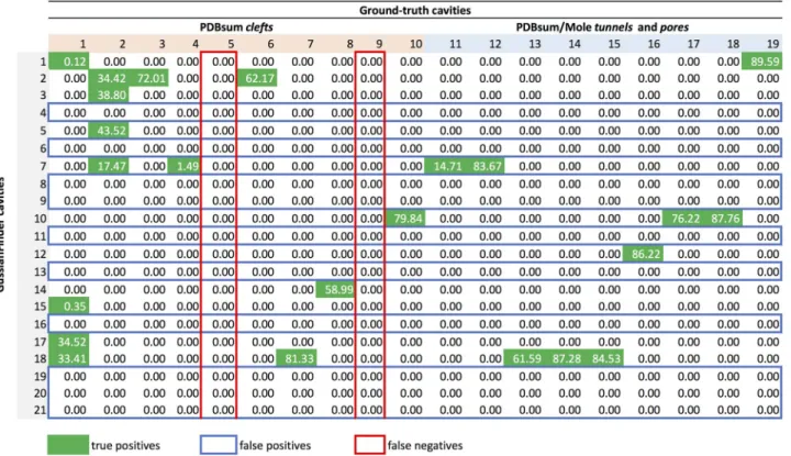
Thus, our cavity overlapping evaluator produces anoverlapping matrix for each protein, as
shown inFig 6, where rows represent method-specific cavities and columns the ground-truth cavities; the first ten columns concern PDBsum clefts, and the remaining columns indicate PDBsum/Mole tunnels and pores. Taking into consideration that CavBench’s dataset includes 2293 proteins, we need to produce 2293 overlapping matrices to evaluate the performance of each cavity detection method. A 3D representation of part of an overlapping matrix depicting the overlapped volumes between cavities detected by the method and those from the ground-truth can be seen inFig 7.
Statistical classifier. As illustrated inFig 5, the statistical classifier computes the number
of true positives (TP), false positives (FP), and false negatives (FN) from the overlapping matrix of each protein. Atrue positive is a hit, that is, a cavity cidetected by a specific method
that overlaps at least one ground-truth cavityCjof a given protein, i.e.,ci\Cj6¼⌀. For
exam-ple, inFig 6, we see that the cavityc14detected by GaussianFinder for the protein 180L is a
true positive because its Jaccard similarity index relative to the ground-truth cleftC8is 58.99%.
Furthermore,c14does not overlap any other ground-truth cavity, so there is no repetition to
consider. On the contrary,c2overlaps three ground-truth cavities, namely the cleftsC2,C3, Fig 6. The overlapping matrix produced by the cavity overlapping evaluator for the protein 180L, as a result of benchmarking the cavities outputted by the GaussianFinder against the ground-truth dataset. Columns correspond to ground-truth cavities and rows to cavities detected by the GaussianFinder method. True positives (TP) correspond to rows (GaussianFinder cavities) containing at least a green cell; false positives (FP) are identified by rows (GaussianFinder cavities) without any green cell, i.e., they do not meet any ground-truth cavity; false negatives (FN) are identified by columns (i.e., ground-truth cavities) in red. This example contains 11 TP (rows), 10 FP (rows) and 2 FN (columns).
andC6, in a scenario with repetitions. Obviously, discarding the repetitions, we would keepC3
because it is the most similar toc2, with a Jaccard index of 72.01%.
Afalse positive is a method-specific cavity that does not overlap any ground-truth cavity.
For example,c4inFig 6is a false positive because it does not intersect any ground-truth cavity.
Therefore, we identify false positives by zeroed rows (only zeros) of the overlapping matrix or, equivalently, cavities detected by the method, but that do not exist in the ground-truth.
Afalse negative is a ground-truth cavity that is not detected by the method. For example,
the cavityC9is a false negative because it does not intersect any method-specific cavity for the
given protein. False negatives can be recognized by zeroed columns, which denote cavities existing in the ground-truth, but not detected by a specific method.
The computation oftrue negatives (TN) is a bit more complex. A true negative is a protein
cavity that is not part of the ground-truth nor is detected by a specific method for a given pro-tein. This means that true negatives cannot be inferred from the overlapping matrix associated to a given protein. These true negative cavities are important because they can be seen as unknown binding sites, which eventually will be sites for binding new drugs or ligands. The
Fig 7. Overlapping matrix (top) and voxelized,cross-eyed stereoscopic 3D visualization of the protein 1A4U. The example represents the overlap between 5 method-detected cavities (rows) and 10 ground-truth cavities (columns). The overlapped portions of the ground-truth cavities are rendered with opaque colors (true positives), and the non-overlapped portions as semi-transparent (false negatives). This example shows that the method detected roughly 13.6% of the first cavity (red), 1.5% of the second (orange), 2.3% of the fourth (light green), 1.4% of the sixth (cyan), and 11.8% of the eigth (purple).
procedure of computing true negatives for each method is as follows: (i) determine the convex hull of the protein; (ii) construct the union that comprises protein atoms, ground-truth cavity pseudo-atoms, and method-specific cavity pseudo-atoms; (iii) construct the difference between such convex hull (first step) and union (second step); (iv) apply DBSCAN to form undetected cavities from the empty difference space. Nevertheless, our statistical study focuses on positive (rather than negative) samples, so we end up not to compute TNs at all.
Performance evaluator. As illustrated inFig 5, CavBench evaluates the performance of a
given cavity detection method (e.g., Fpocket) through three metrics: precision (p), recall (r),
and F-score (F).
Theprecision is a measure of the performance of a given cavity detection method. It is
defined by the number of correctly identified cavities divided by the number of all identified cavities of a specific cavity detection method, that is:
p ¼ TP
TP þ FP ð1Þ
Therecall is also known as sensitivity, true positive rate, or probability of detection, and is
given by
r ¼ TP
TP þ FN ð2Þ
whereTP + FN is the number of positive samples. In the context of protein cavity detection,
the recall measures the rate (or percentage) of positives that are correctly identified by a spe-cific method.
The previous two metrics (precision and recall) do not depend on the number of true nega-tives, that is, they both apply to the positive class. TheF-score combines precision and recall
metrics into a single performance metric for each cavity detection method. Specifically, the F-score is the harmonic mean of precision and recall [56], that is,
F ¼ 2TP
2TP þ FP þ FN ð3Þ
Thus, what determines whether a method performs better than another is its higher value of F-score. In fact, a brief glance at Tables1and2shows us that Fpocket and GaussianFinder perform better than the GHECOM and KVFinder because their F-score values are higher than those of the latter ones. Furthermore, Fpocket generally performs better than GaussianFinder, particularly when we do not consider repetitions.
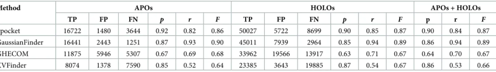
Table 1. Classification (TP, FP, FN) and performance (p, r, F) results with repetitions. Four cavity detection methods are benchmarked against the ground-truth: Fpocket, GaussianFinder, GHECOM, and KVfinder.
Method APOs HOLOs APOs + HOLOs
TP FP FN p r F TP FP FN p r F p r F Fpocket 16722 1480 3644 0.92 0.82 0.86 50027 5722 8699 0.90 0.85 0.87 0.90 0.84 0.87 GaussianFinder 16441 2443 1251 0.87 0.93 0.90 45011 7939 2964 0.85 0.94 0.89 0.86 0.94 0.89 GHECOM 11875 5946 5307 0.67 0.69 0.68 33962 19566 13917 0.63 0.71 0.67 0.64 0.70 0.67 KVFinder 8074 1378 7590 0.85 0.52 0.64 23385 3643 19885 0.87 0.54 0.67 0.86 0.53 0.66 Abbreviations:
APOs: apo proteins; HOLOs: holo proteins.
TP: true positives; FP: false positives; FN: false negatives. p: precision; r: recall; F: F-score.
Results
As suggested by the CavBench workflow shown inFig 5, we end up getting three types of results for each cavity detection method: overlapping matrices (one per protein), classification results, and performance results. These results can be all retrieved from CavBench since we provide the entire method-specific dataset (e.g., the set of all xxxx-GaussianFinder .xml files, one per protein, where xxxx denotes the alphanumeric identifier of each protein) beforehand. Optionally, results for a single protein or a small set of proteins can be also retrieved in the .csv file format.
Overlapping results
By default, the overlapping matrices (one per protein) generated by CavBench for a cavity detection method provide raw results, that is, results with repetitions. In other words, not all method-specific cavitiesciestablish a one-to-one relationship with ground-truth cavitiesCj.
A brief glance atFig 6shows us that the overlapping matrix concerning the protein 180L exhibits rows where a single method-detected cavity overlaps more than one ground-truth cav-ity. That is, overlapping results inFig 6include repetitions. For example,c2intersects three
ground-truth cavities,C2,C3, andC6; in this case, the repetitions (c2,C2) and (c2,C6) are
thrown away (i.e., their overlapping percentages withc2are set to zero) becauseC3is the
ground-truth cavity that most overlapsc2, with a percentage of 72.01%. Likewise,C2is
over-lapped by four method-specific cavities,c2,c3,c5, andc7, butc5is the one that most overlaps
C2, with overlapping percentage of 43.52%; consequently, the overlapping percentages of (c2,
C2), (c3,C2), and (c7,C2) are set to zero. Obviously, as explained below, removing repetitions
alter the classification results in terms of TP, FP, and FN. Hence, we considered two scenarios for results, with and without repetitions (see Tables1and2).
Classification results
The classification results are expressed in terms of the number of TP, FP, and FN, and are obtained from the overlapping matrices associated with the proteins.Table 1lists such results with repetitions for Fpocket, GaussianFinder, GHECOM, and KVFinder, whileTable 2 pres-ents the results without repetitions for the same four methods. By comparing the classification results of both Tables1and2, we see that the removal of repetitions decreases the number of true positives, and increases the number of false positives and false negatives. For example, looking again atFig 6, we see thatc5is a true positive because it is the the cavity that most Abbreviations:
APOs: apo proteins; HOLOs: holo proteins.
TP: true positives; FP: false positives; FN: false negatives. p: precision; r: recall; F: F-score.
overlaps or resemblesC2; so, setting the overlapping percentage of (c3,C2) to zero originates a
new false positive and, consequently, decrements the number of true positives. Furthermore, eliminating the repetitions may also lead to the increase of the number of false negatives and, at the same time, decreasing the number of true positives. For example, removing the repeti-tion (c7,C4) creates a new false negative and decrements the number of true positives.
Performance results
As usual, there are two methodologies to discuss the performance of a given method based on its results. The first methodology consists in findingprecision values when the recall varies in
the interval [0, 1], or vice-versa. The second methodology is more straightforward, and con-sists in combining both scores into a single measure. In either methodology, precision and recall scores are discussed jointly, not in isolation. Here, we have adopted the second method-ology by computing theF-score, which, as mentioned above, is the harmonic mean of precision
and recall.
The performance results are presented in Tables1and2considering both scenarios with and without repetitions, respectively. Note that performance results are better for the scenario with repetitions than without repetitions. For example, the F-score of GaussianFinder takes on the value of 0.89 considering repetitions, and 0.34 without repetitions. In fact, as seen above, discarding repetitions has the effect of reducing the number of true positives (TP) and increas-ing the number of false positives (FP) and false negatives (FN), while keepincreas-ing the same total numbers of method-detected and ground-truth cavities, and thus changing the values of preci-sion, recall, and F-score as given by Eqs (1)–(3).
Precision. In the scenario with repetitions (Table 1), Fpocket is more precise than
any other method; that is, it is capable of correctly identifying more cavities (relative to all identified cavities) than the remaining methods. In fact, considering apo and holo proteins altogether, its precision is 0.90 (in the interval [0, 1]), while the precision values of Gaussian-Finder, GHECOM, and KVFinder are 0.86, 0.64, and 0.86, respectively. Note that Fpocket also performs more precisely than the other three methods in the scenario without repetitions (Table 2).
Recall. A brief glance at Tables1and2allows us to observe that the probability of a
method to correctly detect positives is higher for the scenario with repetitions than without repetitions. In addition, such a probability (i.e., recall) is consistently higher for GaussianFin-der than any other method. In fact, we see that GaussianFinGaussianFin-der ranks first with a joint probability of detection (for apo and holo proteins) of 0.94, while Fpocket, GHECOM, and KVFinder come next with 0.84, 0.70, and 0.53, respectively. However, this ranking does not hold in the scenario without repetitions, as Fpocket performs better than any other method concerning recall, which takes on the value of 0.39.
F-score. By blending precision and recall into a single score, called F-score, we end up
having only one metric to measure the performance of each cavity detection method. Based on the results shown in Tables1and2we see that GaussianFinder performs better than any other method in the scenario with repetitions (F = 0.89), while Fpocket ranks first in the scenario
without repetitions (F = 0.42), considering apo and holo proteins as a whole.
CavBench software
CavBench is available athttps://github.com/mosqueteer/CavBench/. It was designed as a standalone software suite to run entirely on Linux, Mac OSX, and Windows (via Power Shell) using shell scripting. Its idea is to easily and quickly compare any new technique against
state-workflow shown inFig 5. Thus, the XML design of CavBench reinforces the interoperability between distinct operating systems and their versions. Besides,CavBench does not require
installing or compiling programs in some remote execution environment. These features make theCavBench suite easy to run and its results more readily accessible to the research
community.
Conclusions
Identifying cavities on protein surfaces is an important step to both drug design and discovery, and protein docking. So far, researchers have used ad-hoc methods to compare each new cav-ity detection method against known binding sites. This has made it difficult to assess the rela-tive strengths and limitations of new techniques, since there is no common ground against which to evaluate new research. To the best of our knowledge, no benchmark has been pro-posed in the literature to allow comparing cavity detection methods to one another or relative to a ground-truth dataset. We designed CavBench as such a benchmark to fill that gap.
As future work, we intend to also consider true negatives in our benchmark, as well as new metrics to account for the negative class. Furthermore, we plan to add more method-specific datasets (i.e., more methods) and ground-truth datasets to CavBench. We also plan to paralle-lize CavBench’s workflow using GPUs, as well as to create a graphical user interface and add more data visualization tools to provide a more friendly and interactive user experience while affording better insights into comparing method performances.
Acknowledgments
We are grateful to reviewers for their criticism that allowed us to improve this paper significantly.
Author Contributions
Conceptualization: Se´rgio Dias, Tiago Simões, Francisco Fernandes, Abel J. P. Gomes.
Data curation: Se´rgio Dias, Tiago Simões, Francisco Fernandes, Alfredo Ferreira.
Formal analysis: Tiago Simões, Francisco Fernandes, Ana Mafalda Martins, Alfredo Ferreira.
Investigation: Se´rgio Dias, Ana Mafalda Martins, Abel J. P. Gomes.
Methodology: Tiago Simões, Ana Mafalda Martins, Alfredo Ferreira, Joaquim Jorge.
Project administration: Joaquim Jorge.
Software: Se´rgio Dias, Tiago Simões, Francisco Fernandes, Alfredo Ferreira.
Supervision: Abel J. P. Gomes. Validation: Abel J. P. Gomes.
Writing – original draft: Joaquim Jorge, Abel J. P. Gomes.
Writing – review & editing: Francisco Fernandes, Ana Mafalda Martins, Alfredo Ferreira,
Joaquim Jorge, Abel J. P. Gomes.
References
1. Laskowski R, Hutchinson E, Michie A, Wallace A, Jones M, Thornton J. PDBsum: a Web-based data-base of summaries and analyses of all PDB structures. Trends in Biochemical Sciences. 1997; 22 (12):488–490.https://doi.org/10.1016/s0968-0004(97)01140-7PMID:9433130
2. de Beer T, Berka K, Thornton J, Laskowski R. PDBsum additions. Nucleic Acids Research. 2014; 42 (D):292–296.https://doi.org/10.1093/nar/gkt940
3. Kellenberger E, Muller P, Schalon C, Bret G, Foata N, Rognan D. sc-PDB: an annotated database of druggable binding sites from the Protein Data Bank. Journal of Chemical Information and Modeling. 2006; 46(2):717–727.https://doi.org/10.1021/ci050372xPMID:16563002
4. Kuntz ID, Blaney JM, Oatley SJ, Langridge R, Ferrin TE. A geometric approach to macromolecule-ligand interactions. Journal of Molecular Biology. 1982; 161(2):269–288. https://doi.org/10.1016/0022-2836(82)90153-xPMID:7154081
5. Shoichet B, Kuntz I, Bodian D. Molecular docking using shape descriptors. Journal of Computational Chemistry. 1992; 13(3):380–397.https://doi.org/10.1002/jcc.540130311
6. Dias S, Gomes AJP. GPU-Based Detection of Protein Cavities using Gaussian Surfaces. BMC Bioinfor-matics. 2017; 18:493:1–493:10.
7. Voorintholt R, Kosters MT, Vegter G, Vriend G, Hol WG. A very fast program for visualizing protein sur-faces, channels and cavities. Journal of Molecular Graphics. 1989; 7(4):243–245.https://doi.org/10. 1016/0263-7855(89)80010-4PMID:2486827
8. Ho CW, Marshall G. Cavity search: An algorithm for the isolation and display of cavity-like binding regions. Journal of Computer-Aided Molecular Design. 1990; 4(4):337–354.https://doi.org/10.1007/ BF00117400PMID:2092080
9. Caprio C, Takahashi Y, Sasaki S. A new approach to the automatic identification of candidates for ligand receptor sites in proteins: (I). Search for pocket regions. Journal of Molecular Graphics. 1993; 11 (1)23–29.https://doi.org/10.1016/0263-7855(93)85003-9
10. Kleywegt GJ, Jones TA. Detection, delineation, measurement and display of cavities in macromolecular structures. Acta Crystallographica. 1994; 50, Part 2:178–185.https://doi.org/10.1107/
S0907444993011333PMID:15299456
11. Edelsbrunner H, Facello M, Fu P, Liang J. Measuring proteins and voids in proteins. In: Proceedings of the 28th Hawaii International Conference on System Sciences (HICSS’95). Washington, DC, USA: IEEE Computer Society; 1995. p. 256–264.
12. Voss NR, Gerstein M. 3V: cavity, channel and cleft volume calculator and extractor. Nucleic Acids Research. 2010; 38:W555–W562.https://doi.org/10.1093/nar/gkq395PMID:20478824
13. Zhu H, Pisabarro MT. MSPocket: an orientation-independent algorithm for the detection of ligand bind-ing pockets. Bioinformatics. 2011; 27(3):351–358.https://doi.org/10.1093/bioinformatics/btq672PMID: 21134896
14. Schneider S, Zacharias M. Combining geometric pocket detection and desolvation properties to detect putative ligand binding sites on proteins. Journal of Structural Biology. 2012; 180(3):546–550.https:// doi.org/10.1016/j.jsb.2012.09.010PMID:23023089
15. Oliveira SHP, Ferraz FAN, Honorato RV, Xavier-Neto J, Sobreira TJP, de Oliveira PSL. KVFinder: steered identification of protein cavities as a PyMOL plugin. BMC Bioinformatics. 2014; 15(197):1–8. 16. Czirja´k G. PrinCCes: Continuity-based geometric decomposition and systematic visualization of the
void repertoire of proteins. Journal of Molecular Graphics and Modelling. 2015; 62:118–127.https://doi. org/10.1016/j.jmgm.2015.09.013PMID:26409191
17. Kim B, Lee JE, Kim YJ, Kim KJ. GPU Accelerated Finding of Channels and Tunnels for a Protein Mole-cule. International Journal of Parallel Programming. 2016; 44(1):87–108.https://doi.org/10.1007/ s10766-014-0331-8
18. Xenarios I, Rice DW, Salwinski L, Baron MK, Marcotte EM, Eisenberg D. DIP: the Database of Interact-ing Proteins. Nucleic Acids Research. 2000; 28(1):289–291.https://doi.org/10.1093/nar/28.1.289 PMID:10592249
19. Bader GD, Hogue CW. BIND—a data specification for storing and describing biomolecular interactions, molecular complexes and pathways. Bioinformatics. 2000; 16(5):465–477.https://doi.org/10.1093/ bioinformatics/16.5.465PMID:10871269
23. Puvanendrampillai D, Mitchell JB. Protein Ligand Database (PLD): additional understanding of the nature and specificity of protein-ligand complexes. Bioinformatics. 2003; 19(14):1856–1857.https://doi. org/10.1093/bioinformatics/btg243PMID:14512362
24. Gold ND, Jackson RM. SitesBase: a database for structure-based protein-ligand binding site compari-sons. Nucleic Acids Research. 2006; 34(suppl. 1):D231–D234.https://doi.org/10.1093/nar/gkj062 PMID:16381853
25. Hu L, Benson ML, Smith RD, Lerner MG, Carlson HA. Binding MOAD (mother of all databases). Proteins: Structure, Function, and Bioinformatics. 2005; 60(3):333–340.https://doi.org/10.1002/prot. 20512
26. Benson ML, Smith RD, Khazanov NA, Dimcheff B, Beaver J, Dresslar P, et al. Binding MOAD, a high-quality protein ligand database. Nucleic Acids Research. 2008; 36(D):2977–2980.
27. Lopez G, Valencia A, Tress M. FireDB–a database of functionally important residues from proteins of known structure. Nucleic Acids Research. 2007; 35(suppl. 1):D219–D223.https://doi.org/10.1093/nar/ gkl897PMID:17132832
28. Ito JI, Tabei Y, Shimizu K, Tsuda K, Tomii K. PoSSuM: a database of similar protein-ligand binding and putative pockets. Nucleic Acids Research. 2012; 40(D):D541–D548.https://doi.org/10.1093/nar/ gkr1130PMID:22135290
29. Singh H, Chauhan JS, Gromiha MM, Raghava GPS. ccPDB: compilation and creation of data sets from Protein Data Bank. Nucleic Acids Research. 2012; 40(D):D486–D489.https://doi.org/10.1093/nar/ gkr1150PMID:22139939
30. Kufareva I, Ilatovskiy AV, Abagyan R. Pocketome: an encyclopedia of small-molecule binding sites in 4D. Nucleic Acids Research. 2012; 40(D1):D535–D540.https://doi.org/10.1093/nar/gkr825PMID: 22080553
31. Yang J, Roy A, Zhang Y. BioLiP: a semi-manually curated database for biologically relevant ligand-pro-tein interactions. Nucleic Acids Research. 2013; 41(D):D1096–D1103.https://doi.org/10.1093/nar/ gks966PMID:23087378
32. Desaphy J, Rognan D. sc-PDB-Frag: A Database of Protein-Ligand Interaction Patterns for Bioisosteric Replacements. Journal of Chemical Information and Modeling. 2014; 54(7):1908–1918.https://doi.org/ 10.1021/ci500282cPMID:24991975
33. Kawabata T, Go N. Detection of pockets on protein surfaces using small and large probe spheres to find putative ligand binding sites. Proteins: Structure, Function, and Bioinformatics. 2007; 68(2):516– 529.https://doi.org/10.1002/prot.21283
34. Kalidas Y, Chandra N. PocketDepth: A new depth based algorithm for identification of ligand binding sites in proteins. Journal of Structural Biology. 2008; 161(1):31–42.https://doi.org/10.1016/j.jsb.2007. 09.005PMID:17949996
35. Capra JA, Laskowski RA, Thornton JM, Singh M, Funkhouser TA. Predicting protein ligand binding sites by combining evolutionary sequence conservation and 3D structure. PLoS Computational Biology. 2009; 5(12):e1000585.https://doi.org/10.1371/journal.pcbi.1000585PMID:19997483
36. Kawabata T. Detection of multiscale pockets on protein surfaces using mathematical morphology. Pro-teins: Structure, Function, and Bioinformatics. 2010; 78(5):1195–1211.https://doi.org/10.1002/prot. 22639
37. Volkamer A, Griewel A, Grombacher T, Rarey M. Analyzing the Topology of Active Sites: On the Predic-tion of Pockets and Subpockets. Journal of Chemical InformaPredic-tion and Modeling. 2010; 50(11):2041– 2052.https://doi.org/10.1021/ci100241yPMID:20945875
38. Guo F, Wang L. Computing the protein binding sites. BMC Bioinformatics. 2012; 13(10):S2.https://doi. org/10.1186/1471-2105-13-S10-S2PMID:22759425
39. Lo YT, Wang HW, Pai TW, Tzou WS, Hsu HH, Chang HT. Protein-ligand binding region prediction (PLB-SAVE) based on geometric features and CUDA acceleration. BMC Bioinformatics. 2013; 14 (Suppl 4).https://doi.org/10.1186/1471-2105-14-S4-S4
40. Conte LL, Ailey B, Hubbard TJP, Brenner SE, Murzin AG, et al. SCOP: a Structural Classification of Pro-teins database. Nucleic Acids Research. 2000; 28(1):257–259.https://doi.org/10.1093/nar/28.1.257 PMID:10592240
41. Hendlich M, Bergner A, Gu¨nther J, Klebe G. Relibase: design and development of a database for com-prehensive analysis of protein-ligand interactions. Journal of Molecular Biology. 2003; 326(2):607–620. https://doi.org/10.1016/s0022-2836(02)01408-0PMID:12559926
42. Wang R, Fang X, Lu Y, Wang S. The PDBbind Database: Collection of Binding Affinities for Protein-Ligand Complexes with Known Three-Dimensional Structures. Journal of Medicinal Chemistry. 2004; 47(12):2977–2980.https://doi.org/10.1021/jm030580lPMID:15163179
43. Liu Z, Li Y, Han L, Li J, Liu J, Zhao Z, et al. PDB-wide collection of binding data: current status of the PDBbind database. Bioinformatics. 2014; p. btu626.
44. Dessailly BH, Lensink MF, Wodak SJ. LigASite: a database of biologically relevant binding sites in pro-teins with known apo-structures. Acid Nucleic Research. 2008; 36:D667–673.https://doi.org/10.1093/ nar/gkm839
45. Saito T, Rehmsmeier M. The Precision-Recall Plot Is More Informative than the ROC Plot When Evalu-ating Binary Classifiers on Imbalanced Datasets. PLoS ONE. 2015; 10(3):1–21.https://doi.org/10. 1371/journal.pone.0118432
46. Laskowski RA. SURFNET: A program for visualizing molecular surfaces, cavities, and intermolecular interactions. Journal of Molecular Graphics. 1995; 13(5):323–330.https://doi.org/10.1016/0263-7855 (95)00073-9PMID:8603061
47. Petřek M, Kosˇinova´ P, Koča J, Otyepka M. MOLE: A Voronoi Diagram-Based Explorer of Molecular Channels, Pores, and Tunnels. Structure. 2007; 15(11):1357–1363.https://doi.org/10.1016/j.str.2007. 10.007PMID:17997961
48. Le Guilloux V, Schmidtke P, Tuffery P. Fpocket: an open source platform for ligand pocket detection. BMC Bioinformatics. 2009; 10(1):1–11.https://doi.org/10.1186/1471-2105-10-168
49. Sehnal D, Vařekova´ RS, Berka K, Pravda L, Navra´tilova´ V, Bana´sˇ P, et al. MOLE 2.0: advanced approach for analysis of biomacromolecular channels. Journal of Cheminformatics. 2013; 5(1):39. https://doi.org/10.1186/1758-2946-5-39PMID:23953065
50. Ester M, Kriegel HP, Sander J, Xu X. A density-based algorithm for discovering clusters in large spatial databases with noise. In: Simoudis E, Han J, Fayyad U, editors. Proceedings of the Second Interna-tional Conference on Knowledge Discovery and Data Mining (KDD’96). AAAI Press; 1996. p. 226–231. 51. Forgy EW. Cluster analysis of multivariate data: efficiency versus interpretability of classifications.
Bio-metrics. 1982; 21(3):768–769.
52. Lloyd SP. Least square quantization in PCM. IEEE Transactions on Information Theory. 1982; 28 (2):129–137.https://doi.org/10.1109/TIT.1982.1056489
53. Brady GP, Stouten PFW. Fast prediction and visualization of protein binding pockets with PASS. Jour-nal of Computer-Aided Molecular Design. 2000; 14(4):383–401.https://doi.org/10.1023/
A:1008124202956PMID:10815774
54. Huang B, Schroeder M. LIGSITEcsc: predicting ligand binding sites using the Connolly surface and degree of conservation. BMC Structural Biology. 2006; 6(1):19.https://doi.org/10.1186/1472-6807-6-19 PMID:16995956
55. Weisel M, Proschak E, Schneider G. PocketPicker: analysis of ligand binding-sites with shape descrip-tors. Chemistry Central Journal. 2007; 1(1):7.https://doi.org/10.1186/1752-153X-1-7PMID:17880740 56. Powers D. Evaluation: From Precision, Recall and F-Measure to ROC, Informedness, Markedness and