Universidade Nova de Lisboa - Faculdade de Ciências e Tecnologia Department of Computer Science

(1)

Universidade Nova de Lisboa - Faculdade de Ciências e Tecnologia

Department of Computer Science

SOLAP+:

Extending the Interaction Model

By Ruben Jorge

Thesis submitted to Faculdade de Ciências e Tecnologia of the Universidade Nova de Lisboa, in partial fulfillment of the requirements for the degree of Master in Computer Science

Supervisor: PhD João Moura Pires

(2)

(3)

Abstract

Decision making is a crucial process that can dictate success or failure in today’s businesses and organizations. Decision Support Systems (DSS) are designed in order to help human users with decision making activities. Inside the big family of DSSs there is OnLine Analytical Processing (OLAP) - an approach to answer multidimensional queries quickly and effectively.

Even though OLAP is recognized as an efficient technique and widely used in mostly every area, it does not offer spatial analysis, spatial data visualization nor exploration. Geographic Information Systems (GIS) had a huge growth in the last years and acquiring and storing spatial data is easier than ever. In order to explore this potential and include spatial data and spatial analysis features to OLAP, Bédard introduced Spatial OLAP (SOLAP). Although it is a relatively new area, many proposals towards SOLAP’s standardization and consolidation have been made, as well as functional tools for different application areas.

(4)

(5)

Resumo

A tomada de decisões é um processo crucial que pode ditar o sucesso ou insucesso dos negócios e organizações de hoje. Os Sistemas de Apoio à Decisão (SAD) são desenhados de modo a ajudar os utilizadores humanos nas actividade de tomada de decisões. Dentro da grande família dos SAD está o Processamento Analítico Online (OLAP) - uma aproximação para dar resposta a consultas multidimensionais de modo rápido e eficaz.

Ainda que OLAP seja reconhecido como uma técnica eficiente e amplamente utilizada em praticamente qualquer área, esta não oferece análise espacial, visualização de dados espaciais nem exploração. Os Sistemas de Informação Geográfica (SIG) tiveram um crescimento enorme nos últimos anos e adquirir e armazenar dados espaciais é mais fácil que nunca. De modo a explorar este potencial e incluir dados espaciais e funcionalidades de análise espacial em OLAP, Bédard introduziu o Spatial OLAP (SOLAP). Apesar de ser uma área relativamente nova, várias propostas no sentido de criar standards e consolidar SOLAP têm sido efectuadas, assim como ferramentas funcionais para diferentes áreas de aplicação.

(6)

(7)

Agradecimentos

Ao Professor Doutor João Moura Pires, pela aposta em mim para este projecto e por tudo o que me ensinou, não só relativamente à área de investigação mas também no sentido de manter um espírito crítico, rigor e exigência.

Ao António Cruz e ao Pedro Lopes pelo tempo disponibilizado e apoio com questões técnicas durante o desenvolvimento da tese.

A todos os colegas e amigos de faculdade, que de um modo ou de outro me ajudaram ao longo deste percurso. Um agradecimento especial ao Francisco Costa, meu amigo e colega de trabalho ao longo de seis anos e que me ajudou sempre que precisei.

Ao pessoal da OCHC, por terem provado ao longo dos anos os amigos que são, por todas as aventuras e discussões que me ajudaram a crescer.

(8)

(9)

ix

Figure Index

Figure 1 - A Star Schema ... 6

Figure 2 - A Snow Flake ... 6

Figure 3 - Geometry Class Hierarchy from OpenGIS Features ... 11

Figure 4 - Types of spatial dimensions based on the levels’ data type ... 12

Figure 5 - Classification of topological relationship for aggregation procedures (Malinowsky and Zimányi) ... 14

Figure 6 - StatCan interface ... 16

Figure 7 - The Spatial One base framework ... 17

Figure 8 - Alternative 1 ... 18

Figure 9 - Alternative 2 ... 19

Figure 10 - An aggregate navigator... 21

Figure 11 - The extended framework ... 25

Figure 12 - Data representation on the extended framework ... 26

Figure 13 - Four combinations of different spatial attributes values leading to four partitions ... 27

Figure 14 - Example partition and respective vector object (vObj) ... 28

Figure 15 - Geometric Grouping Function ... 29

Figure 16 - Map and support table after SOLAP operations - The semantic attribute "Region" is presented on (...) ... 31

Figure 17 - An example support table displaying one numerical measure ... 32

Figure 18 - Example of representation of one single numerical measure using color and legend ... 34

Figure 19 - Chart showing "Population" as a numerical measure and ordered by a hidden function "Area" (...) ... 35

Figure 20 - Support table ordered by hidden function "Area" (ascending order) (Source: INE) ... 35

Figure 21 - Selected point and auxiliary distance lines... 36

Figure 22 - Support table ordered by hidden function "Distance to point X" (ascending order) (Source: INE) ... 36

Figure 23 - Chart showing "Crime Rate" as numerical measure and ordered using hidden function "Distance to (...) .... 36

Figure 24 - Support table at lower detail level (Source: INE) ... 37

Figure 25 - Detail table at higher detail level (Source: INE) ... 37

Figure 26 - Detail chart example (Source: INE) ... 38

Figure 27 - Example support table with two numerical measures ... 38

Figure 28 - Example of combination of charts and colors to represent four numerical measures ... 39

Figure 29 - Selected values for clustering algorithm (feature vectors)... 40

Figure 30 - Example support table for clustering ... 40

Figure 31 - Clusters discovered ... 41

Figure 32 - Clusters represented by color ... 41

Figure 33 - Support table and respective chart when there is no active selection... 42

Figure 34 - Support table and respective chart when selecting a line ... 42

Figure 35 - Support table and respective chart when selecting a column (measure) ... 43

Figure 36 - Support table and respective chart when selecting two lines and two columns (measures) ... 43

Figure 37 - An example support table with year attribute ... 44

Figure 38 - Support table for two semantic attributes from semantic dimensions and one numerical measure ... 44

Figure 39 - Support table for one semantic attribute from semantic dimension and two numerical measures ... 44

Figure 40 - An example map where a numerical measure is represented along with 3 distinct values (...) ... 46

Figure 41 - Support table after adding sA ... 47

Figure 42 - Map with numerical measure and semantic attribute representation ... 48

Figure 43 - Support table after adding store_type (sA) ... 48

Figure 44 - Hierarchy diagrams ... 49

(13)

xiii

Figure 46 - Portuguese administrative subdivisions ... 51

Figure 47 - "Município" subdivision - lowest data granularity ... 51

Figure 48 - "Distrito" subdivision ... 52

Figure 49 - "NUTS II" subdivision ... 52

Figure 50 - Verifying the inclusion principle ... 53

Figure 51 - Intersections between "Distrito" and "NUTS II" ... 53

Figure 52 - Support table ... 54

Figure 53 - Map (with legend) ... 54

Figure 54 - Example of support table and respective map when representing two spatial attributes (...) ... 55

Figure 55 - Example of support table and respective map when representing two spatial attributes (...) ... 56

Figure 56 - Alternative representation ... 56

Figure 57 - Example using relationship-lines ... 57

Figure 58 - New support table with aggregated data ... 57

Figure 59 - New map representation ... 58

Figure 60 - New map representation using charts ... 58

Figure 61 - Support table and map representation without visualization clustering ... 59

Figure 62 - Support table and map representation with visualization clustering ... 59

Figure 63 - Table representation ... 61

Figure 64 - Tree representation ... 61

Figure 65 - Possible and recommended visualization styles... 62

Figure 66 - SOLAP+ Logical Architecture ... 66

Figure 67 - SOLAP+ Server Architecture ... 67

Figure 68 - Server’s Data Request Processor Architecture ... 68

Figure 69 - Levels organized in hierarchies... 70

Figure 70 - Relationships between two levels ... 70

Figure 71 - The all level ... 71

Figure 72 - Two incomparable levels ... 71

Figure 73 - SOLAP+ Client Architecture ... 73

Figure 74 - Client's Data Processor Architecture ... 74

Figure 75 - Meta Model Root Element ... 80

Figure 76 - MapViewer's Architecture (Extracted from Pro Oracle Spatial) ... 90

Figure 77 - Implementation Overview ... 92

Figure 78 - SOLAP+ Request Lifecycle ... 93

Figure 79 - Support Table Structure ... 96

Figure 80 - SOLAP+ Client Interface ... 97

Figure 81 - Interface with both tables minimized and hidden right panel ... 98

Figure 82 - Dimensions panel where “Emissao” dimension and “Poluente” level are expanded ... 98

Figure 83 - A typical SOLAP+ session with all panels expanded ... 99

Figure 84 - Map Control detail example ... 99

Figure 85 - Slice panel with an active slice ...100

Figure 86 - Dialog box for creating/editing a slice ...100

Figure 87 - Slice panel with an active slider ...101

Figure 88 - Dialog box for creating/editing a spatial slice ...101

Figure 89 - Dialog box for creating/editing a measure filter ...102

Figure 90 - Defining measures and attributes order ...102

Figure 91 - Removing elements from the analysis ...103

Figure 92 - Loading a model/session ...103

Figure 93 - Saving a session ...104

Figure 94 - Data model for the use case ...107

Figure 95 - Spatial hierarchies for dimension Installation ...107

(14)

xiv

Figure 97 - Output example for one measure and a polygon spatial attribute ...109

Figure 98 - Output example for one measure and spatial objects generated by intersection ...110

Figure 99 - Output example for two measures ...111

Figure 100 - Output example when using header attributes ...112

Figure 101 - Output example for two header attributes ...114

(15)

Chapter 1

Introduction

1.1. Context and Motivation ... 2 1.2. Objective and Contributions ... 7 1.3. Thesis Structure ... 8

(16)

Chapter 1 – Introduction

2

This chapter starts by presenting the context and motivations for the elaboration of this thesis, including some introductory information about OLAP and SOLAP. Next, it mentions the objective and contributions of this thesis and finally there is an overview of its structure.

1.1.Context and Motivation

Decision Support Systems (DSS) are a class of computer applications that helps human users with decision making activities on business and other organizations. It is considered that the concept of Decision Support Systems became an independent area of research in mid 1970’s, evolving to a larger scale during the 1980’s. At the conceptual level, Power differentiates DSSs in five different categories [1]:

 A model-driven DSS emphasizes access to and manipulation of a statistical, financial, optimization, or simulation model. Model-driven DSS use data and parameters provided by DSS users to aid decision makers in analyzing a situation, but they are not necessarily data intensive;

 A communication-driven DSS supports more than one person working on a shared task; (collaborative tools);

 A data-driven DSS or data-oriented DSS emphasizes access to and manipulation of a time series of internal company data and, sometimes, external data;

 A document-driven DSS manages, retrieves and manipulates unstructured information in a variety of electronic formats;

 A knowledge-driven DSS provides specialized problem solving expertise stored as facts, rules, procedures, or in similar structures.

Data-driven systems are designed in order to provide decision makers with useful information compiled from the organization’s raw data that will help them choose between alternatives in a given situation. The decision-making process is no longer associated with a single central entity - it is spread across multiple users with different backgrounds and positions. This democratization led to the development of this kind of systems. Data-driven DSSs provide data reasoning operations such as comparison, pattern and outliers finding, tendencies, among others. These operations allow the user to improve his efficiency in problem solving and encourages exploration and discovery.

(17)

Section 1.1 - Context and Motivation

3 While OLAP meets all the requirements for an easy-to-use, fast and intuitive system, it has no support for spatial data visualization and analysis.

Geographic Information System (GIS) is a computer-based information system that enables capture, modeling, storage, retrieval, sharing, manipulation, and presentation of geographically referenced data.

Even though GIS is adequate for most applications that need to display or manipulate geographical data, it does not have the efficiency required from an analysis tool that deals with large amounts of data like OLAP, as Rivest and Bédard mention: “(...) despite interesting spatiotemporal analysis capabilities, it is recognized that actual GIS systems per se are not optimally designed to be used to support decision applications and that alternative solutions should be used” [2].

Nowadays there are large amounts of GIS data available. There are also many techniques to acquire it with increasing accuracy and precision. As more data with higher quality and reliability becomes available, new applications and tools are possible, including the usage of GIS capabilities as tools for analyzing spatial-related data.

It has been estimated that about 80 percent of all data stored in corporate databases are spatial data [3]. This is a clear indicator that spatial data analysis has a very wide application area. This factor along with the advance of GIS tools and DataBase Management Systems (DBMS) supporting GIS data, allowed the development of a new type of tools that combined OLAP and GIS called SOLAP (Spatial OLAP).

Rivest, Bédard et al. defined a SOLAP tool as “a visual platform built especially to support rapid and easy spatio-temporal analysis and exploration of data following a multidimensional approach comprised of aggregation levels available in cartographic displays as well as in tabular and diagram displays” [4]. These tools add spatial analysis and visualization to the standard OLAP interaction.

Several SOLAP tools have been implemented since then, however they are specific to a strict and pre-determined context and of complex usage. This complexity prevents the analysis and consequent decision making process to be made by different users, something that regular OLAP tools achieved through interaction standards and general ease of use. The work of Rosa Matias [5] and subsequent research by Marlene Vitorino and Rodolfo Caldeira [6] led to a generic, although limited, SOLAP interaction model.

(18)

4

1.1.1.Multidimensional Model

Using a multidimensional approach to model a system is enforcing simplicity [7]. A multidimensional model is composed of hypercubes, measures, dimensions, levels, hierarchies and attributes.

Dimensions are used to map and categorize data into entities that are relevant to the organization (such as product, date and warehouse in a retail sales model). Attributes are the characteristics of these dimensions (such as name, description and price in product dimension).

Each dimension can index data at several detail/aggregation levels. Hierarchies can then be defined using the levels of a dimension. For example, the date dimension can have day, week, month, year as a hierarchy and month, trimester, year as another.

A hypercube is a logical structure that has the organization's data indexed by the dimensions. Each of its cells represents an intersection from all the dimensions and contains measures – values associated to this relationship.

“The simplicity of the model is inherent because it defines objects that represent real-world business entities. Analysts know which business measures they are interested in examining, which dimensions and attributes make the data meaningful, and how the dimensions of their business are organized into levels and hierarchies.” [8]

1.1.2.Data Granularity

Regarding data granularity, Joe Oates says in DMReview [9]: “Granularity refers to the level of detail of the data stored fact tables in a data warehouse. High granularity refers to data that is at or near the transaction level. Data that is at the transaction level is usually referred to as atomic level data. Low granularity refers to data that is summarized or aggregated, usually from the atomic level data. Summarized data can be lightly summarized as in daily or weekly summaries or highly summarized data such as yearly averages and totals.”

Data granularity is a very important point in a data warehouse and data analysis. Typical OLAP operations use several data granularity levels in order to summarize and present data to the user. In order to aggregate data, an aggregation operator is needed for each measure: sum, average, etc for numerical measures; union, intersection, etc for spatial measures.

1.1.3.Typical OLAP Operations

(19)

Section 1.1 - Context and Motivation

5 analyst to focus on the relevant data. For example, if the analyst is interested in data from January 2009 only, he will apply a slice operation on the time dimension, selecting rows where the year attribute is equal to '2009' and month is equal to 'January'.

A user can filter data based on measure values, excluding elements that do not match the required criteria (Example: “Consider only sales of over 1,000 units”). Selection operations relative to measure values are also possible, such as Top/Bottom X elements. Along with slice, this enables queries such as “What were the top 10 selling products on Lisbon region in 2008?”. Note that filtering is applied before data is aggregated, while top/bottom operations are applied after.

Data aggregation levels are changed using two operations: Roll-up and drill-down. Roll-up consists on summarizing or aggregating data by going up a hierarchy towards the least detailed level. Drill-down is the opposite operation, going Drill-down a hierarchy towards the most detailed level. By using drill-down operations, the analyst can understand the reasons behind summarized data. By using roll-up operations, the analyst can see the impact of the facts on a larger scale. As an example, consider a minimalist multidimensional model of a sales company containing two dimensions: product and time. The lowest data granularity represents the sale of a certain product at a certain time. To the store manager, a monthly report detailing the sales of each product in each hour, wouldn't be very helpful for his decision making process. Probably a report depicting sales per product type and per week (roll-up) would be more reasonable. However, if the analyst detects an abnormal sales amount on one of those weeks, he may perform a drill-down operation to explain the data at a lower level (product, day or hour) in order to detect the cause.

1.1.4.OLAP Modes

There are three different modes for storing cubes in a data warehouse: Multidimensional OLAP (MOLAP), Relational OLAP (ROLAP), and Hybrid OLAP (HOLAP).

In MOLAP data is stored in multidimensional cubes built for fast data retrieval. Aggreations are pre-calculated, meaning that response times are very good. Also because of this pre-calculation, it can only handle a limited amount of data. This can be countered by pre-calculating only part of the aggregations.

In ROLAP, the underlying data is stored in a relational database with multiple related tables. It's conceptual model gives the appearance of traditional OLAP operations such as slicing and roll-up/drill-down using the dimensions. It can handle large amounts of data but it has slower response times. It is also limited by the SQL functionalities when executing queries. To address this limitation there are extensions to the SQL language especially designed to deal with multidimensional models.

(20)

6

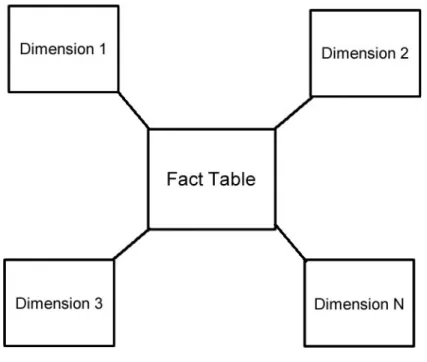
There are two main ways of arranging tables when using a ROLAP approach: Star-schema and snowflake schema. The star-schema (see Figure 1) is the simplest one and it consists of fact tables (or just one) referencing multiple dimension tables.

Figure 1 - A Star Schema

In the snowflake schema (Figure 2), the fact tables are also centralized and reference dimension tables, but dimensions are normalized into multiple related tables, resembling a snowflake.

(21)

Section 1.2 - Objective and Contributions

7

1.1.5.SOLAP Challenges

SOLAP poses a lot of challenges. Some of those are shared with standard OLAP tools but it also has specific ones that were not an issue before.

Semantic and spatial data integration

Integrating spatial and non-spatial data is the base for a SOLAP tool. This integration poses several issues regarding how and where to store both types of data (data structures, databases vs GIS, pointers to spatial data, etc) in order to work together as a single tool.

Performance

A fast response to queries is a critical requirement for OLAP tools and its importance to SOLAP is not lower. Because SOLAP deals with spatial data and operations, an acceptable response time is harder to achieve, since those operations usually involve much more processing and thus more time to perform than those using regular data.

Ease of use

Being easy to use is a very important characteristic for an analysis tool, especially when it is designed to be used by different classes of users. This allows the user to focus on the actual data analysis rather than how to do it. Dealing with maps and other geographical information poses another obstacle to interface design and user interaction.

Standardization

Defining standards is an approach to support innovation, increasing productivity and assuring the quality of a product or group of related products. SOLAP standards are far from being reached - Lots of subjects are still under discussion or reasearch and several different methods are proposed for the same objective such as multidimensional models for spatial data, spatial measures, spatial hierarchies, interaction models, topological operators, etc.

1.2.Objective and Contributions

The objective of this thesis is to extend the generic SOLAP interaction model by including new components on the base framework and redefining the interaction and presentation on the different cases and scenarios. The initial models’ limitations are presented as well as the new proposal to overcome them and extend its capabilities. An architecture for such a system and a prototype to exemplify some of the features proposed in the interaction model will also be developed.

(22)

8

 SOLAP Interaction Model - Extending and improving:

o Visualization components

o Interaction cases

o Analysis options

 Metamodel for SOLAP - A new proposal that allows the usage of aggregates in order to improve performance

 Prototype - An application that partially implements the proposed features in the interaction model:

o General

o Easy to use

o Flexible

o Aggregate-aware

1.3.Thesis Structure

The content of this thesis is structured in seven chapters and one annex. Follows the listing and description of each chapter:

(23)

Chapter 2

State of the Art

2.1. Geometrical Data Types in DBMS ... 10 2.2. Multidimensional Models for Spatial Data ... 12 2.3. SOLAP Systems ... 15 2.4. Clustering ... 19 2.5. Aggregate Navigators ... 20 2.6. Other Works on Spatial Perfomance ... 21 2.7. Conclusion ... 21

(24)

Chapter 2 – State of the Art

10

The introduction of spatial data can be a huge step in the decision making process of many organizations, even those already using conventional OLAP tools for their spatio-temporal analysis. With a plain OLAP tool, analysts don’t have the features to visualize spatial data, perform spatial analysis or explore the data using a map. [4].

It has been estimated that about 80 percent of all data stored in corporate databases is spatial data [3]. Among these large numbers is a wide variety of areas onto which spatial analysis could be applied: Airline companies that work with plane routes, railroad companies dealing with tracks, phone operators registering calls’ origins and destinations, pharmaceutical companies knowing the locations of hospitals, health centers, etc. [5].

Even though SOLAP is a relatively new area of research, there have been important works that are slowly leading to its applicability and standardization. Some researchers have managed to define many concepts related to spatial data and several multidimensional models have been proposed.

Next in this chapter we will give an overview on previous work on geometrical data types, operations and their implementation on conventional DBMSs that eventually allowed spatial data analysis to progress. The next section refers works on multidimensional models for spatial data - the base foundation for SOLAP tools, including spatial dimensions, hierarchies and measures. We will then present SOLAP systems/generic interaction models already existent and the possible usage of clustering in those tools.

2.1.Geometrical Data Types in DBMS

An entity is geographic if it has attributes that are associated with the earth coordinate system. These entities can have two kinds of components: semantic or descriptive attributes and spatial attributes. For example, a county has attributes that represent it’s name, population, unemployment rate, etc (semantic) and attributes that depict its boundaries, cities, etc (spatial).

DataBase Management Systems were initially designed and optimized to deal with simple alphanumeric data. With the growth of GIS and the expansion of available spatial data, DBMSs started to include structures to handle this kind of data. It is required that the spatial module of a DBMS has the following properties [5]:

 Abstract types for spatial data - The possibility to create conceptual and logical models using spatial data

 Spatial query language - It is necessary that the SQL language is extended in order to handle spatial data

(25)

Section 2.1 - Geometrical Data Types in DBMS

11 required that optimized mechanisms be developed and implemented in order to efficiently execute spatial queries.

The Open Geospatial Consortium (OGC) was founded in 1994 by a group of both public and private organizations with the intent of promoting development and usage of non-proprietary norms or standards on spatial data processing. To do this, the OGC develops and revises specifications where protocols and interfaces are described.

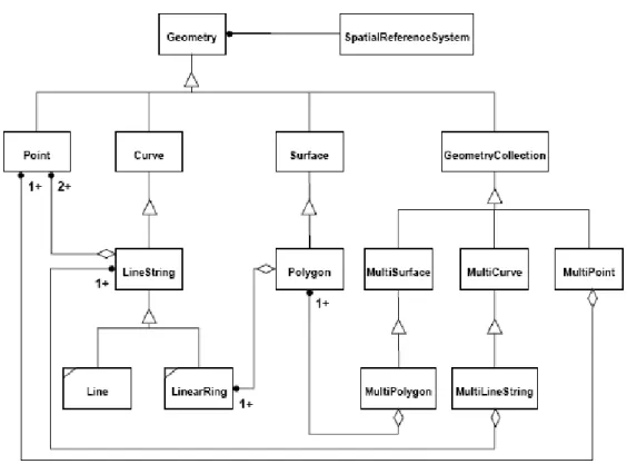
The OpenGIS Simple Feature Specification for SQL [10] is an OGC specification that contains a norm defining spatial objects in a class diagram (see Figure 3). From the abstract class Geometry derives Point, Curve, Surface and GeometryCollection.

Point is used to describe objects with zero dimensions, such as city locations on a map. Curve is used to represent objects like roads or rivers. Surface enables us to represent regions, areas or any other two-dimensional objects such as counties, natural reservations, etc. GeometryCollection allows more complex objects resulting from the combination of multiple objects by using spatial functions such as union, intersection, etc.

Figure 3 - Geometry Class Hierarchy from OpenGIS Features

(26)

12

and distance functions. Some of these functions are general for all kinds of geometries (returning the description of a geometry type) but most of them are specific for each type - returning the X coordinate of a point (Point), returning the length of a curve (Curve), return the area (Surface), etc.

2.2.Multidimensional Models for Spatial Data

Even though multidimensional models have been used for data analysis for a long time and have solid foundations, the introduction of spatial data requires a rethinking of the concepts associated with it, mainly those related to dimensions, hierarchies and measures.

The usage of spatial dimensions allows the analyst to execute new and powerful slices using topological operators for example “Amount of fishing products sales in shops that are within a 5 km buffer of a river or lake”, “What is the crime rate percentage in districts that are at least 2 km away from a police station?”, “Return the top 10 plants on CO2 emissions that are inside a protected region“, etc.

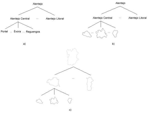
Several works [4][2][11][12] categorize spatial dimensions based on the type of data on each of its hierarchy levels: a) Non-geometric (when all levels contain only descriptive data); b) geometrical to non-geometrical (when the finest granularity levels contain geometrical data and the coarser granularity levels contain descriptive data) and c) fully geometrical (when all the levels contain geometrical data only). These types are depicted in Figure 4:

(27)

Section 2.2 - Multidimensional Models for Spatial Data

13 Fidalgo et al. [11] proposed a framework to be used as guidance for designing geographical dimensional schemas, considering geographical (only geographical attributes) and hybrid (geographical and conventional attributes) dimensions. It includes modeling guidelines in order to minimize redundancy of spatial data by normalizing Composed Geographical Dimensions (a dimension with multiple spatial attributes) into Primitive Geographical Dimensions (one that contains only one spatial attribute).

Spatial dimension hierarchies and the associated aggregation/summarization issues are subject to research in some works [13][11][14][15]. In particular, Malinowsky and Zimányi [13] defined different kinds of spatial hierarchies and gave a conceptual model for them. The summarizability problems that arises for some of those hierarchies is also studied. The conceptual model for the hierarchies is simple and effective, covering relationships between levels (denoted by child and parent) and respective cardinalities, spatial data types and topological relationships. Using real-world examples/applications, a generic classification of hierarchies (both spatial and non-spatial) is defined: Simple, Non-Strict, Multiple and Parallel.

Simple spatial hierarchies are those where the relationships between their members can be represented as a tree, for example a hierarchy depicting a relationship between stores, counties and states. Symmetric hierarchies have at the schema level only one path where all levels are mandatory. This implies that, at the instance level, the members form a tree where all the branches have the same length. Asymmetric hierarchies have only one path at the schema level but some of the lower levels of the hierarchy are not mandatory, causing the members at the instance level to generate a non-balanced tree. Generalized hierarchies contain multiple exclusive paths sharing some levels among them. At the instance level, each member belongs to only one path.

Non-strict spatial hierarchies are those that have at least one many-to-many cardinality. The previous hierarchy types can also be non-strict in addition to their already defined type. Most of the non-strict hierarchies arise when a partial containment relationship exists (only part of a river belonging to a county for example).

Multiple alternative spatial hierarchies have multiple non-exclusive simple spatial hierarchies sharing some levels. At the instance level, these hierarchies form a graph, since a child member can be associated with more than one parent member belonging to different levels.

Parallel spatial hierarchies arise when a dimension has multiple spatial hierarchies for different analysis criteria. In a parallel independent hierarchy, hierarchies do not share levels, as opposed to a parallel dependent hierarchy.

(28)

14

based on the result of the intersection between the geometric union of the spatial extent of child members and the spatial extent of their associated parent member.

Figure 5 - Classification of topological relationship for aggregation procedures [13]

The same authors also proposed a conversion for this multidimensional model into an object-relational schema, based on SQL [16]. In this article, examples of spatial functions including aggregation functions can also be found.

The usage of spatial measures is a widely discussed subject far from having a standard defined, both on when and how to apply them. In the works that address this subject, there are three main approaches on how to define spatial measures:

1) Using the concept of geographical measure: an entity described by geometric, metric and thematic (textual) attributes. Complex aggregation functions must be defined for these entities since multiple attributes may need to be aggregated using different functions [17][18][14][19]. An example of a geographical measure using this approach would be the following element:

{Name = “Region1”; Shape = (PolygonCoordinates); Type = “A”; MeasureValue = “100”}

2) As a numerical value that is calculated by applying a spatial or topological operator like area or distance to an existent geometric object [16][2]. In this case, a spatial measure could be: SUM(Region1.area() + Region2.area())

(29)

Section 2.3 - SOLAP Systems

15 Several problems related to spatial measure aggregations arise. Different aggregation functions are required, since there are different data types (spatial and semantic) with distinct meanings for each measure. To deal with the geometric part of a measure, a spatial aggregation function is needed in order to receive possibly multiple objects as input and return a single object as the output. This function can become especially complex and ineffective when the geometric objects are themselves calculated using spatial operations, causing a chain of time-costly geometric operations.

In conclusion, in most of the studied works, the geometric part of the spatial measure is an existent object or a new one computed based on existent ones from spatial dimensions – either a county, region or any other logical of administrative boundary. The only slight reference to an arbitrary geometric shape directly and solely related to a fact is present in a work by Matias and Moura-Pires [20]. In this work, an arbitrary spatial measure is proposed to represent the pollutant emission cloud as a polygon. The emission cloud is only related to the event of an emission, not to any spatial attribute or hierarchy from the dimensions.

2.3.SOLAP Systems

Bédard et. al. [4] defined and presented the features of a SOLAP system in three main areas: Visualization of Data, Exploration of Data and Structure of Data.

Under Visualization of Data, the authors defend the need for cartographic and non-cartographic displays, and their flexibility, either by using multiple displays at the same granularity or at different levels. The representation of multiple measures is another focused point as well as an interactive legend that allows the user to visualize numerical information at different levels while remaining at the same spatial level. The importance of using charts and guidelines for their construction is discussed by Tufte [21] and MacEachren [22]. Usage of context information is encouraged as it helps the user locate the displayed information.

Related to Exploration of Data, the authors explain the need for the availability of the data exploration operations in all display types, both cartographic and non-cartographic; availability of both topological and metric functions for data analysis and a timeline component for manipulating the temporal dimension. Also in this section is placed emphasis on calculated measures (measures calculated from other measures stored in the cube), filtering on the dimension members (slicing operations) and the display of significant data aggregates only, by eliminating irrelevant or empty cells from the aggregation process.

(30)

16

data (changing over time) and support for different data sources, mainly the three OLAP modes (MOLAP, ROLAP, HOLAP) are also noted.

Even though this work provides many important guidelines for the development of SOLAP applications, it lacks detail on how to model and implement the proposed features throughout the article.

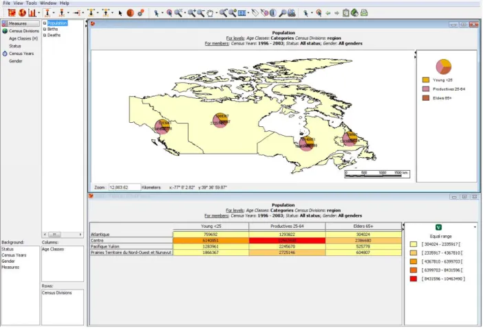
2.3.1. StatCan

StatCan [23] is a tool to analyze data from the Census of Canada. The usual census data is available such as age, gender, residence status, etc. The main SOLAP tools are available: slice, roll-up and drill-down. It includes several possible measures such as population, births and deaths.

Figure 6 - StatCan interface

The interface (see Figure 6) contains a panel for the map and one for the table. At any time the analyst can request a chart based on the information presented. In that case, a new panel is opened and the related chart is presented.

(31)

Section 2.3 - SOLAP Systems

17 The map offers the possibility to display multiple numerical measures by using charts associated with each region. It also has the basic features of zoom, spatial selection and labeling.

Slice operations are made by selecting one or more values for each attribute. Roll-up and drill-down operations can be made on either the map panel or the table panel. Applying those operations to one panel causes the other one to adapt its representation to the appropriate granularity level and executing the necessary summarization.

2.3.2.The Spatial One

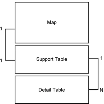
Vitorino, M. and Caldeira, R. developed a generic SOLAP interaction model [6] based on a previous interaction model by Matias, R. [5]. They defined both the components and the behavior of the system based on several generic interaction cases from the user. Those interaction cases are the base for any specific SOLAP application that may use the generic model defined. This model features the usage of spatial slices mentioned before, namely the possibility to slice by distance to a certain point, by topological operator (such as “contained in”, “touches”, ...) and by the top/bottom elements (ex.: “the 10 nearest factories to river X”).

The base framework proposed has three main components: The map, the support table and the detail table (Figure 7).

Figure 7 - The Spatial One base framework

(32)

18

The support tableis used to show the base data from which the map representation depends. This includes attributes from dimensions (semantic attributes) and measures.

The detail table is a tool to provide the user with more in-depth analysis. In order to maintain the 1:1 relationship between the support table and the map, drill-down operations resulting in certain detail levels should not be expressed in the support table, because they can’t be represented in the map (The 1:1 relationship need is explained further on). In these cases, the detail table is used to analyze that data at a lower aggregation level.

Any one of the three components can also show numerical measures.

The 1:1 relationship between the map and the support table is an important property that should be kept in any situation. It helps the analysis process as to each spatial object on the map, there is a corresponding line in the support table.

To justify this property we have to look at the alternatives to a 1:1 relationship. Those are: 1. Multiple lines in the support table to one spatial object on the map (Figure 8)

In this case, we would have multiple rows associated with each spatial object. Selecting a spatial object in the map would select multiple rows, possibly spread along the table, making it difficult for the user to relate the information in the table to the objects on the map.

Figure 8 - Alternative 1

2. One line in the support table to multiple spatial objects in the map (Figure 9)

(33)

Section 2.4 - Clustering

19 Figure 9 - Alternative 2

Data in the support table is usually aggregated at a certain level. However, if the user requires a more in-depth analysis, he/she can use the detail level, where the same data is shown but at a lower level of aggregation. This means that for each line in the support table, we will possibly have multiple lines in the detail table that represent the same data, thus the 1:N relationship.

Using this framework, the authors defined a generic interaction model contemplating the following cases:

1. One numerical measure 2. Multiple numerical measures

3. Using semantic attributes from semantic dimensions 4. Using semantic attributes from spatial dimension 5. Using spatial attributes from the same dimension 6. Using spatial attributes from different dimensions

2.4.Clustering

Even though clustering is not directly related to the SOLAP area, it will have a very important role in our interaction model proposal, used at several levels and with different goals, as we will explain further on.

Data analysis is a process that requires ease of use and fast response times so that the user can maintain his train of thought. The amount of data presented to the user and its level of detail is also extremely important: Too much or too detailed data presented at one time to the user will prevent him from drawing conclusions.

(34)

20

To address this problem we propose clustering or merging nearby spatial objects into groups represented by a single entity on the map. These groups have no semantic meaning and the spatial objects they contain are similar only on their geographical position, so that would be the only feature to be used as an input parameter on the clustering algorithm.

CLARANS [24] is a k-medoid clustering algorithm which identifies circular clusters based on a distance function. Each point is assigned to the cluster to which the distance to its respective k-medoid point has the smaller value. This algorithm requires an input parameter K – the number of clusters to be generated. Since we are only considering grouping by geographical proximity, circular clusters identified by CLARANS seems to be adequate in this case.

Clustering techniques can also be used to discover similar elements based on their associated measures. Note that in this case the geographical location is not relevant, only the measures related to them.

DBSCAN [25] is a density-based clustering algorithm that relies on notions of core and border points to determine which points belong to which cluster. Since it is density-based and not distance-based like CLARANS, it generates clusters with arbitrary shapes and doesn’t need an input parameter specifying the number of clusters to generate. In order to identify clusters based on feature vectors, DBSCAN is more accurate (as it does restrict itself to circular clusters) and with better response times than CLARANS. It is adequate for clustering needs that are not location/geography based, such as identifying similar elements based on multiple measures.

More recent works [26][27] aim to define techniques and algorithms for clustering spatial objects. Those can be interesting for simplifying visualization when dealing with polygons.

2.5.Aggregate Navigators

According to Ralph Kimball [28], providing a proper set of aggregate records is the best way to improve performance of a data warehouse. These aggregate records are summarized records obtained from the original data. Since they are summarized, operations over them are faster than having to compute all the original records.

(35)

Section 2.6 - Other Works on Spatial Performance

21 Figure 10 - An aggregate navigator

The SQL generated by the end-user application always refers the base multidimensional model’s fact tables and dimensions - it is the responsibility of the aggregate navigator to convert that base SQL into aggregate-aware SQL, where aggregate tables are referenced in case a usable aggregate is present.

2.6.Other Works on Spatial Performance

Even though this issue is not within the scope of our work, we believe a few considerations on this are important. Response time is a major concern in any analysis tool: Users expect to be able to see the results of their requested operations in timely fashion, allowing him to maintain his train of thought. An already crucial issue to a standard OLAP tool is taken to an even higher level when dealing with SOLAP, since manipulating spatial data is usually much more time costly.

Stefanovic et. al. [31] proposed time efficient methods for computing spatial measures, merging spatial objects and selecting pre-aggregated cuboids based on an adapted greedy algorithm for spatial databases.

Papadias et. al. [32] presented a method that uses aggregation trees based on Minimum Bounding Rectangles to discover arbitrary spatial hierarchies. These newly discovered hierarchies are then added to a greedy algorithm that will decide which pre-aggregates to materialize.

Spatial operations are very time costly, both on I/O and CPU. In order to minimize the cost of polygon amalgamation operations, an algorithm that reduces the number of polygons used in those operations to the absolute minimum was developed [33]. This algorithm works by identifying the internal polygons which would not be used in the amalgamation process. Two methods can be used for this identification, polygon adjacency or spatial indexes.

2.7.Conclusion

In order to achieve standard levels for SOLAP, there is still much to be done. Even though there are several proposals for most of the issues presented, many of those proposals are not compatible with each other, leading to the development of specific applications rather than generic interaction models or tools. Spatial measures is a particular case of an issue with different and incompatible proposals which has a lot of open possibilities to explore.

(36)

(37)

Chapter 3

Extended Interaction Model

3.1. Multidimensional Model Concepts and Extended Framework ... 24 3.2. Data Representation ... 26 3.3. Interaction Cases Overview ... 31 3.4. One Numerical Measure ... 32 3.5. Multiple Numerical Measures ... 38 3.6. Semantic Attributes from Semantic Dimensions ... 43 3.7. Semantic Attributes from a Spatial Dimension ... 46 3.8. Spatial Attributes from One Dimension ... 48 3.9. Spatial Attributes from Two Dimensions (or with no inclusion) ... 54 3.10. Spatial Measures ... 59 3.11. Visualization Complexity ... 60 3.12. Styles and Legend ... 62

(38)

Chapter 3 – Extended Interaction Model

24

Our work proposal is to extend the generic SOLAP interaction model previously presented [6]. We aim to redefine the behavior on several interaction aspects as well as adding new components to the visualization and new interaction cases that were not considered before.

This chapter starts by introducing a few concepts related to our multidimensional model and presenting our extended framework components followed by an explanation on how data is represented. An overview of the considered interaction cases is then presented. Finally, each of the interaction cases is exposed in detail.

3.1.Multidimensional Model Concepts and Extended Framework

We consider two types of dimensions in our model, depending on what kind of data they contain: Semantic dimensions and Spatial dimensions.

A dimension is constituted by levels. These levels are organized within one or more hierarchies inside the dimension and each level can contain multiple attributes. Levels can be compared with each other, being higher or lower in case they are on the same hierarchy or incomparable if they are on different hierarchies. This issue is addressed on section 4.3 when studying aggregates.

A dimension is semantic if it has semantic attributes only. If the dimension has at least one spatial attribute, then it is considered a spatial dimension.

Definition 1: Semantic attribute (sA) is a textual or numerical attribute from a dimension.

Definition 2: Spatial attribute (spA) is an attribute from a dimension containing a coordinate or group of coordinates that represent a spatial object. Each spatial attribute has an associated semantic attribute used to represent it in a table or another textual component. The associated semantic attribute to a spatial attribute is represented as sA(spA).

Definition 3: Spatial object (spO) is a GIS element that is either a point (ex.: client location), line (ex.: road) or polygon (ex.: county). It is not necessarily connected to a dimension.

Our interaction model considers the two most common multidimensional model architectures: Star Schema and Snow Flake. The fact table is where the relationships between the dimensions as well as possible measures are present. Measures can also be of two kinds: Numerical measures and spatial measures.

(39)

Section 3.1 - Multidimensional Model Concepts and Extended Framework

25 Definition 5: Spatial measure (spM) is a coordinate or group of coordinates that represent a spatial object. It is associated with a fact and stored in the fact table. Note that these are arbitrary spatial measures only, as mentioned in section 2.2.

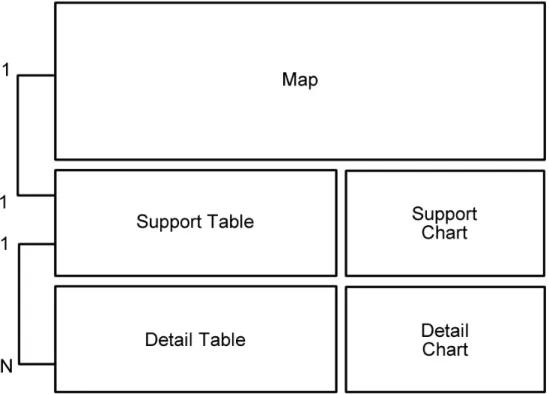
The extended framework we propose (see figure below) has two new components and some changes to the previous ones on how information is presented. The new components are the support chart and the detail chart.

Figure 11 - The extended framework

The map is used to present reference maps, spatial objects and other SOLAP information to the user.

The support table is used to show textual and numerical data at the same granularity as the map. This includes attributes from dimensions and measures. The detail table is a tool to provide the user with more in-depth analysis, usually at a finer granularity level by applying drill-down operations to the data in the support table.

The support chart is a tool used to visualize data referring to the support table. The detail chart is related to the data in the detail table.

(40)

Chapter 3 26 3.2.Dat The fra granularity coarser lev The two where Que rowsets -

3 – Extended

ta Repre

amework co y levels at vel while the

o required ery 2 is the

a set of ro

Interaction M

sentatio

omponents the same t e detail tab

Figure

data sets e result of a ows where

Model

on

s are used time. The m ble and deta

12 - Data rep

(low and h a drill-down each one

to repres map, suppo ail chart do i

presentation o

high detail) n operation

refers to a

ent data i ort table an

it at a finer

on the extend

are obtain over Query a combinat

n different nd support

level, as we

ded framewor

ned by exe y 1. This da tion of attr

t ways and chart pres e can see in

rk

ecuting data ata comes i ributes (bot

d at differe sent data a n Figure 12:

abase quer in the form th spatial a

ent t a

(41)

semantic) for the res In our i associated map and t object into Pre-pro (discussed The ne created, w one of thes

Each gr )(Figu

defined in pective attr interaction with a sin the support o one. In ord ocessing (1)

below) is a xt step is p where is th se groups w

Figure 13

roup is the ure 14):

an SQL GRO ribute comb model, we gle spatial t table. Thi der to do th is optional n example) partitioning he number o will represen

- Four combin

en convert

OUP BY clau bination. e introduce

object, wh is is done b his, the rows ly applied t ) by creating

(2) the row of combina nt a spatial

nations of dif

ed into a

use. These

e the possib ile maintain by merging set returne to the query

g virtual row wset return

tions betwe object. See

fferent spatial

vector (3)

rows also c

bility of rep ning the on g multiple r

d is subject y data set (C ws from the

ed after ex een spatial e Figure 13 f

l attributes va

that repre

Sect contain the

presenting ne to one r rows that r t to several Clustering f e original on xecuting the attributes’ for an exam

alues leading

esents an o

tion 3.2 - Data selected m

multiple n relationship

efer to the transforma for visualiza nes.

e query: g values in th mple of parti

to four partit

object (vec

a Representat measure valu

umeric valu p between t e same spat

tions: ation purpos

groups will he query. Ea

(42)

28

Figure 14 - Example partition and respective vector object (vObj)

These transformations are not required for the detail components - the vector objects are directly obtained from the lower granularity rowset. Having multiple rows referring the same spatial object is not a problem in these cases because for each element in the higher level components (map, support table, support chart) there are N elements in the lower level components (detail table and chart), allowing a more in-depth analysis.

Each component has a specific representation function. A representation function (RF) is a function that maps a set of vector objects ({ }) to a visual representation on a certain component, namely map RF (mRF), support table RF (stRF), support chart RF (scRF), detail table RF (dtRF) and detail chart RF (dcRF):

({ })

According to the component, the output from the respective representation function will be a spatial object on the map (Map), a line on a table (Support table, Detail table) or a chart (Support chart, Detail chart). All these functions take a sub-set of the vectors’ elements as input. While presenting the interaction cases, the input of the representation functions will be adapted to the given scenarios.

(43)

Section 3.2 - Data Representation

29 There are however, two particular cases of the representation function: The first case is when each vector object can be represented individually, without the need for any other information, for instance, a row in the detail table. This representation function could be defined as:

({ }) = ∑ ( ), where ∑ () represents the successive call of a representation function for each vector object.

The second particular case is when each vector object can be represented individually but requiring some context information; an example would be a bar in a chart - it can be represented individually but it would require a maximum and minimum scale value, both of which are context variables, not information from the object itself. This representation function could be defined as:

({ }) = ∑ ( , ({ })), where ∑ () represents the successive call of a representation function for each vector object and ({ }) is the context information, previously extracted from the global set.

As mentioned before, there are three high granularity and two low granularity representation functions, one for each component: Map, Support Table and Support Chart as higher level visualization components and Detail Table and Detail Chart as lower level components. The following sub-sections describe those representation functions.

3.2.1.Map Representation Function (mRF)

The different types of parameters taken by the representation functions determine different spatial object properties on the map. The selected sub-set of the spatial attributes in the rowset determines the location of the respective spatial object on the map. If only one spatial attribute is used, then its location is determined by the spatial attribute’s plain coordinates. If more than one spatial attribute is used in the representation function, an additional spatial object is computed using a Geometric Grouping Function ( ) that takes multiple spatial attributes as input. Then, the new spatial object’s coordinates determine its location on the map. can be defined as: ( , … , ) ( ), where is the number of spatial attributes used in the representation function (see Figure 15).

(44)

30

varies depending on the interaction case: It can be a spacial intersection, union, difference or any other function that generates a spatial object from multiple spatial objects. Representing only one spatial object on the map for each element ensures the 1:1 relationship between the support table and the map explained above.

The selected sub-set of the rowset’s semantic attributes and measures determines the color, pattern, shape, associated chart or any other characteristic regarding that spatial object.

In the simplest case we would have one spatial attribute representing a point and one measure. A single point would be marked on the map (at the same coordinates as the ones from the spatial attribute) with a certain color or size (determined by the measure value).

The most complex case would be multiple spatial attributes that represent polygons and multiple measures and/or semantic attributes. In this case we have more than one spatial attribute, therefore would be used, taking those spatial attributes as input and returning a representative spatial object. Then, the representation function takes all the measures/semantic attributes and determines the new object’s color, associated chart, pattern, etc.

Slicing and filtering the data for analysis is a crucial step in any OLAP/SOLAP interaction. However, even after executing those operations, the map representation when dealing with multiple spatial attributes can still be complex. To minimize this problem we propose using clustering algorithms and grouping/aggregating data sets based on their spatial location. Those ad-hoc groups do not have any semantic meaning other than being geographically near each other. Groups can be created or decomposed by user interaction or automatically related to zoom variation. This group generation is also the responsibility of , even though it’s results have to be available to the other components, in order to maintain the consistency among the represented data.

3.2.2.Support Table Representation Function (stRF)

maps a set of vector objects to a table representation. In most cases, this representation function falls into the first particular case presented above, where it can be decomposed into multiple representation functions, each of them mapping a vector object individually. This is not the case when using visualization clustering for example. In this case we would need the general approach of mapping the entire set of vectors.

(45)

Figure

It is also This helps As mention

3.2.3.Su

’s it usually c either with

3.2.4.De

The rep , kee by the high

3.3.Inte

There a following c Base sc

1.

2.

16 - Map and m

o very impo the user es ned before, upport Ch

objective is can be deco h some cont etail Rep

presentation ping in min her compon

eraction

are several cases start f cenario: One

One numer = { Multiple nu

= {

d support tabl map to establis

ortant that stablish a co , these asso hart Repr

s to map a s omposed in

text inform resentati

n functions nd that the nents - it is a

n Cases O

representa from a base e spatial att rical measur

, ( umerical me

, (

le after SOLAP sh a connecti

every spat onnection b ociated sem resentati

set of vecto to multiple ation (such ion Func

for the de set of vecto at a lower g

Overview

ation cases e scenario w tribute and re

), } easures

), , … ,

P operations -on to the resp

ial attribute between tho antic attrib ion Funct

or object’s t e calls to a r as chart sty tions (dtR

etail table a or objects t granularity,

w

that we w where intera correspond

}

- The semanti pective line in

e has a ose element utes are re tion (scR

to a visual c representat

yle, size, etc RF and d

nd chart co taken as inp more detai

will address action is app ding seman

Section 3.3

ic attribute "R n the support

an associate ts in the ma presented b F)

chart repres tion functio c) or withou dcRF)

omponents put is not th iled level.

using our plied. tic attribute

3 - Interaction

Region" is pre t table

ed semanti ap and the

by ( )

sentation. J on for each

ut it.

are similar he same as

framework

e is present

n Cases Overv

esented on th

c attribute support tab ).

Just like vector obje

r to a the one us

k. Each of t

(46)

32

Base scenario: One or more numerical measures are present in addition to a spatial attribute and corresponding semantic attribute:

3. Semantic attributes from semantic dimensions

= { , , , … , , , … , }

4. Semantic attributes from spatial dimension

= { , , , … , , , … , }

5. Spatial attributes from the same dimension

= { , , … , , , , … , }

6. Spatial attributes from different dimensions

= { , , … , , , , … , }

The last (7th) group of interaction cases is related to spatial measures.

Even though they are not mentioned in the following interaction cases, the spatial slice possibilities used in the works of Vitorino and Caldeira [6] and mentioned in section 2.3.2 are adopted - distance to a point, topological operators and neighbours (top/bottom).

Some of the given examples use data from Instituto Nacional de Estatística (INE).

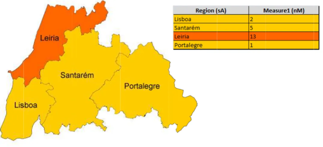
3.4.Case 1: One Numerical Measure

The first interaction case depicts the representation of a single numerical measure associated to a spatial attribute, where = { , ( ), }. ( ) is the semantic attribute associated with the spatial attribute .

3.4.1.Support Table

In the spatial dimensions, for each spatial attribute there is a corresponding semantic attribute . The support table has a column for the semantic attributes and one column for the respective numerical measure. The spatial attribute is not represented in the support table (as you can see in Figure 17), therefore: = ( ( ), ).

(47)

Section 3.4 - Case 1: One Numerical Measure

33 Each line can be colored with the same color from the map’s legend, in order to more easily establish a relation between a line and the corresponding spatial object in the map. The map’s legend component is addressed further on.

3.4.2.Map

As it was pointed out before, the visualization has a one to one relationship with the support, meaning that for each line in the support table, there is a corresponding spatial object on the map.

The representation function for each is then defined as = ( , ( ), ). This function generates a spatial object on the map based on the input values - in this case the spatial object’s properties (such as size, color, etc) are conditioned by the measure value and the type of object (point, line, polygon).

determines each spatial object’s location, while determines the color, shape, size, or any other characteristic that can graphically map a value.

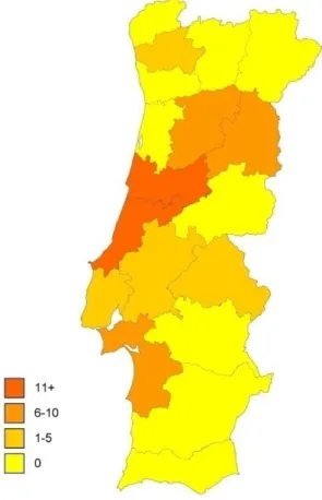
As an example, we will consider is a polygon that represents a Portuguese region. That said, can’t use neither size nor shape as those are relevant for the location. Color has been chosen because it is easy to recognize for the user and it also offers more personalization options than the pattern approach for example. For each spatial object , sets its color to a value that is determined by the respective numerical measure (using a mapping function).

(48)

34

Figure 18 - Example of representation of one single numerical measure using color and legend

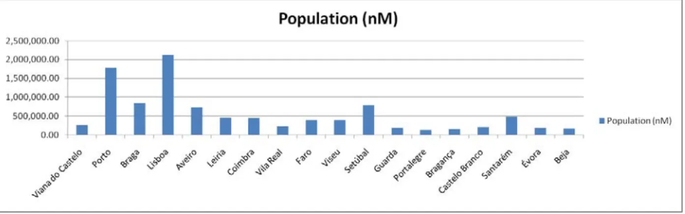
3.4.3.Support Chart

In the extended model, associated with our support table we have a support chart. This component’s function varies with the type and number of attributes and measures being used for the analysis. The support chart representation function ( ) takes a set of vector objects as input ( = { , ( ), }) to produce the chart.

In this case, semantic associated attributes ( ( )) are represented along one axis and numerical measures values ( ) along the other. Besides the possibility to order the chart bars by alphabetic order (semantic attribute), ascending/descending measure value or user-defined, we can also order the chart by the return values of a function not shown in the chart (ℎ ). The values returned by ℎ are represented on the support table.

This function takes one spatial attribute as input and returns an orderable, real number.