UNIVERSIDADE NOVA DE LISBOA
Faculdade de Ciências e Tecnologia
Departamento de Engenharia Electrotécnica e Computadores
M
ICRO
ECG:
A
N INTEGRATED PLATFORM FOR THE CARDIAC
ARRYTHMIA DETECTION AND CHARACTERIZATION
Por
Bruno Ricardo Guerreiro do Nascimento
Dissertação apresentada na Faculdade de Ciências e Tecnologia da Universidade Nova de Lisboa para obtenção do grau de Mestre em Engenharia
Electrotécnica e Computadores
Orientador: Professor Arnaldo Guimarães Batista
Co-orientadores: Professor Manuel Ortigueira
Dr. Luis Brandão Alves
Lisboa
1
Agradecimentos
Esta dissertação não representa só o resultado de extensas horas de estudo, reflexão e trabalho durante vários anos. É também o culminar de um objectivo académico que me propus e que não seria possível sem a ajuda de um vasto número de pessoas, entre as quais gostava de destacar:
O Professor Orientador Arnaldo Batista, ao qual estou profundamente agradecido, não só pela sua perspicácia, conhecimento e habilidade para superar os diversos obstáculos durante a orientação desta dissertação, mas também pela constante disponibilidade, amizade e entusiasmo contagioso.
O Professor Co-orientador Manuel Ortigueira, pelos seus sábios conselhos e recomendações perante as dificuldades encontradas.
O Professor Raul Rato, pelo interesse e disposição em colaborar sempre que solicitada a sua ajuda.
O Dr. Luís Brandão Alves do Hospital Garcia de Orta, pela disponibilidade com que nos recebeu, pelas recomendações apontadas à melhoria do software apresentado e ainda pela nomeação de pacientes que ajudaram à obtenção de resultados práticos.
Ao Carlos Mendes, pela sua disponibilidade e ajuda no desenvolvimento de versões anteriores do software aqui apresentado.
Agradeço também à Isabel Couto e Ana Valente, pela ajuda prestada na aquisição dos electrocardiogramas e por tornarem estas sessões de recolha de dados mais descontraídas.
A todos os voluntários que realizaram o HR-ECG também vai o meu especial apreço pela paciência e disponibilidade apresentada.
Queria ainda agradecer também a todos os Professores, colegas e amigos que encontrei na minha passagem pela Faculdade de Ciências e Tecnologia, de quem recebi sempre simpatia e cujos momentos passados vou sempre transportar comigo.
2
Sumário
O desenvolvimento de um pacote de software para lidar facilmente com electrocardiogramas de alta resolução tornou-se importante para pesquisa na área de electrocardiografia. O desenvolvimento de novas técnicas para detecção de potenciais tardios e outros problemas associados a arritmias cardíacas têm sido objecto de estudo ao longo dos anos. No entanto, ainda existe a lacuna de um pacote de software que facilmente permita implementar algumas destas inovadoras técnicas de uma forma integrada, possibilitando avaliar técnicas clássicas como o protocolo de Simson para a detecção de sinais não estacionários (potenciais tardios). Algumas destas inovadoras técnicas envolvem a detecção tempo-frequência usando escalogramas ou a análise espectral usando metodologias wavelet-packet, sendo implementadas no software desenvolvido com flexibilidade e versatilidade suficientes para que futuramente sirva de plataforma de pesquisa para o refinamento destas mesmas técnicas no que toca ao processamento de sinais de electrocardiogramas de alta resolução. O software aqui desenvolvido foi também desenhado de forma a suportar dois tipos de ficheiros diferentes provenientes de outros tantos sistemas de aquisição. Os sistemas suportados são o ActiveTwo da Biosemi e o USBamp da g.tec.
Abstract
The development of a software package able to easily deal with high-resolution electrocardiograms has became important to the research within the area of electrocardiography. The development of new late potentials detection techniques and other problems associated to cardiac arrhythmia have been studied. However, there is still the need of a software package that can easily implement some of these innovative techniques in an integrated form, allowing the evaluation of some classic techniques such as the Simson’s protocol to the detection of non -stationary signals (late potentials). Some of these innovative techniques are the time-frequency analysis through scalograms and the spectral analysis using the wavelet packet methodologies and they were implemented in the developed software with flexibility and versatility enough to allow, in the future, that this software could be able to be used as a platform to refine these same techniques in a signal processing approach. The developed software was designed to support two different data
3
Symbols and connotations’ inde
x
a– Scale
A – Approximation signal
AC– Alternate current
ADC– Analog to digital conversion
AD-Box– Analog to digital Box
AF– Atrial fibrillation
Ag-AgCl– Silver, Silver Chloride
AIB – Analog input box
aVr, aVl and aVf –Extended unipolar derivations
b – Temporal segment
BDF – Biosemi’s data file
𝐛𝐢(𝐧)- Signal’s noise of n points on the i cycle
BPM – Beats per minute
𝐁𝐰 - Passing band
cA– Approximation signal down sampled
cD– Detail signal down sampled
CMS –Common mode sense
Co2 – Carbon dioxide
CWT– Continuous wavelet transformation
D– Detail signal
DC– Direct current
DI, DII and DIII– Frontal plane bipolar derivations
DRL –Driven right leg
DWT– Discrete wavelet transformation
ECG– Electrocardiogram
ECG(t)– Electrocardiogram in a time domain
EDF– European data format
4
EMG– Electromyography
EP/ERP –Event potential, event related potential
Fc–Wavelet’s central frequency
FFT– Fast Fourier transformation
Fs - Frequency sampling
HR-ECG– High Resolution Electrocardiogram
𝐇 𝐬 - Transfer function in the s plane
𝐇(𝐰)– Butterworth filter transfer function
H(z)– Transfer function in the z plane
I, II and III– Frontal plane bipolar derivations
IIR - Infinite Impulse Response
LAA – left atrial appendage
LAS – Low amplitude signal
LAS40– Time duration where the low amplitude signal reaches the 40 microvolts mark until the end of signal
LSB –Least significant bit
M – Length of the signals of reference cycle and signal to align
MEG/MCG– Microgram
mVpp– milliVolts peak to peak
N – Number of cycles (heart beats)
QRSd - QRS complex time duration
QRSoffset – QRS complex end time
QRSonset – QRS complex start time
R– Reference cycle length
RMS– Root mean square
RMS20– Root mean square value of the last 20 milliseconds
RMS30 - Root mean square value of the last 30 milliseconds
RMS40 - Root mean square value of the last 40 milliseconds
SNR – Signal to noise ratio
RSR – Signal/noise relation
𝐑𝐒𝐑𝐑– Signal/noise relation in R cycles
5
s – s plane
s’ = new s plane
𝐬𝐢(𝐧) - Useful signal of n points on the i cycle
STFT– Short-term Fourier transformation
S-A node– Sino-atrial node
t – Time
V1, V2, V3, V4, V5 and V6– Unipolar thorax derivations
𝐕𝐀– Amplitude vector
𝐕𝐋𝐀–Potential difference in left arm
𝐕𝐋𝐋–Potential difference in left leg
VLPs– Ventricular Late Potentials
𝐕𝐑𝐀–Potential difference in right arm
Vx, Vy and Vz–Frank’s derivations
V-A node– Atrio-ventricular node
𝐰𝟎– Central frequency
xi– Signal of reference cycle
𝐱 –Mean signal
x(t), y(t) and z(t)–Instantaneous amplitudes in the three Frank’s derivations
yi – Signal to align
𝐲 –Reference cycle
z – z plane
Δ - Sampling period of the transformation signal
𝛒– Correlation
𝛔𝐛(𝐧) - Standard deviation of the noise’s value on n points
Ψ – Analyzing wavelet
Ψ(t) – Analyzing wavelet in a time domain
6
Chapter’s Index
1 Objectives ……….….……….…….pg.13
2 Introduction ……….……….…….…….pg.14
2.1 Anatomy……….………..……….………..……….……….pg.14
2.2 Electrocardiography……….…………..……….pg.15
2.3 The heart’sdynamics ………..………..pg.15
2.4 Depolarization sequence ………..………pg.16
2.5 Electrical system………..………..……….pg.17
2.5.1 Electrical pathway ……….………..pg.18
2.6 Nervous control of the heart ………..……..………..pg.18
2.6.1 Accelerator nerves ……….……….…pg.19
2.6.2 Vagus nerve ………..……….pg.19
2.7 Electrical signal and electrocardiography ………..…….…..pg.19
2.7.1 Standard ECG acquisition: the derivations.……….………..………pg.19
2.7.2 Formation of the ECG signal……….……..pg.22
2.7.3 Vectorcardiography……….pg.26
2.8 High Resolution ECG………pg.29
2.8.1 HR-ECG acquisition………..pg.30
2.8.2 Signal Averaging…..………..………..pg.31
3 Cardiac Arrhythmias……….…….pg.35
3.1 Reentrant circuits.………..……….……….pg.35
3.2 Late potentials………pg.35
3.2.1 Ventricular arrhythmia and late potentials…..………..…..pg.36
3.2.2 Atrial arrhythmia and late potentials…..……….……….………..pg.38
4 Late potentials’ detection………..…………pg.40
4.1 Simson’s method..………..……….…….……….……….pg.40
4.2 Magnitude vector’s parameters………..…pg.43
5 Late potentials’ detection using wavelets………pg.45
5.1 Continuous wavelet transformation………....pg.45
5.2 Discrete wavelet transformation and wavelet packets……….…pg.51
7
6.1 Components……….………..pg.56
6.2 Technical specifications………..pg.61
7 Data acquisition………..………pg.62
8 Algorithms……….………..………pg.64
8.1 General processes…………..………..…...pg.64
8.2 Late potential simulator……….pg.65
8.3 Open file………...…pg.66
8.4 Read file……….pg.67
8.5 Peak detection……….…..pg.69
8.6 Show template………..pg.70
8.7 Fine tuning………pg.70
8.8 ECG variability……….………...pg.71
8.9 Heart rate variation………..…………pg.72
8.10 Noise level……….………….pg.72
8.11 Raw data from electrodes……….…..pg.73
8.12 12-lead ECG……….……..pg.73
8.13 Magnitude vectors………..pg.74
8.14 Wavelets……….………….pg.75
9 Interface……….………pg.76
9.1 Introduction to MicroECG……….…….pg.76
9.2 Compilation process………..………..pg.77
9.3 Installation and minimum requirements……….…pg.78
9.4 Instruction manual………..….pg.79
10 Results.………..…pg.109 10.1 Magnitude vectors (Simson’s method for time domain analysis)………..pg.110
10.2 Heart rate variation………..…pg.113
10.3 ECG variability………..……….pg.118
10.4 Wavelet scalograms………pg.121
10.5 Wavelet packets………..……….…………pg.124
11 Conclusions and further work...………..pg.126
8
Figure’s Index
Figure 2.1 - Heart's blood flow………..………….pg.15
Figure 2.2 - Blood entering the heart………..………pg.15
Figure 2.3 - Atrial contraction……….pg.16
Figure 2.4 - Ventricular contraction………..……..pg.16
Figure 2.5 - Human heart in detail. ………..…………..pg.17
Figure 2.6 - Heart's electrical system……….…….pg.17
Figure 2.7 - Willem Einthoven (1906)……….…….pg.19
Figure 2.8 - Front plane bipolar derivations……….………pg.20
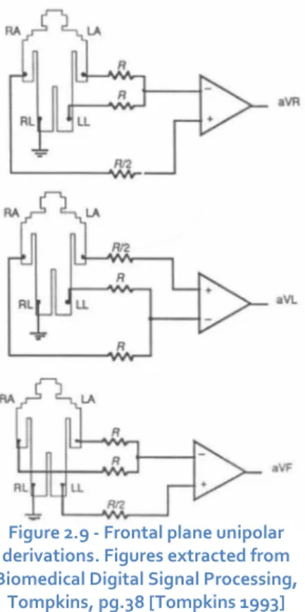
Figure 2.9 - Frontal plane unipolar derivations……….………..……..pg.20
Figure 2.10 - Electrode positioning in the unipolar derivations of the thorax (V1 to V6)………..……….…….pg.21
Figure 2.11– Sequence of the generation of the ECG signal in the Einthoven limb leads……….…….pg.23/24
Figure 2.12 - The normal electrocardiogram………..pg.25
Figure 2.13 - The projections of the lead vectors of the 12-lead ECG system in three orthogonal planes when one assumes
the volume conductor to be spherical homogeneous and the cardiac source centrally located………..…pg.26
Figure 2.14 - The lead matrix of the Frank VCG-system. The electrodes are marked I, E, C, A, M, F, and H, and their anatomical positions are shown. The resistor matrix results in the establishment of normalized x-, y-, and z-component lead vectors, as described in the text………..……pg.27
Figure 2.15– The seven electrode channels obtained through Biosemi’s ActiveTwo acquisition system using the Frank’s
lead VCG system………..……….…..pg.28
Figure 2.16–The three Frank’s derivations (Vx, Vy and Vz) obtained in MicroECG by using the seven electrode channels as
input of the Frank’s VCG equation system………..…….pg.29
Figure 2.17 - HR-ECG electrode positioning……….………..pg.31
Figure 2.18– Noisy signals are often seen even in high quality equipment such as the one used, most of these noise are
due internal factors such as muscular activity or external factors such as environment electromagnetic
noise……….……….pg.33
Figure 2.19– A heart beat template is a smoother signal due to signal averaging……….……..pg.34
Figure 3.1 - Circuit reentry………pg.35
Figure 3.2–Historical picture of a patient’s magnitude vector with positive late potentials on QRS Complex.…………..pg.36
Figure 3.3–MicroECG’s study for the template’s magnitude vector for both the P-wave and the QRS complex. Shown are
ventricular late potentials and their respective parameters values. ……….pg.37
Figure 3.4 - ECG of atrial fibrillation (top) and sinus rhythm (bottom). The purple arrow indicates a P wave, which is lost in
atrial fibrillation………...………pg.38
Figure 3.5–MicroECG’s study for the template’s magnitude vector for both the P-wave and the QRS complex. Shown are
atrial late potentials and their respective parameters values………..…pg.39
9
Figure 4.2 - Transfer function and phase of the fourth order Butterworth's passing-band filter. Marked red there is the passing-band (40 to 250 Hz) on a gain of 0 dB………pg.42
Figure 4.3 - Impulsive response to the fourth order Butterworth filter………..……….pg.42
Figure 5.1 - The wavelet-coefficient calculation is illustrated using a set of analyzing wavelet from the ‘Mexican hat’
wavelet and the ECG signal from a healthy subject. The analyzing wavelets are first multiplied by the ECG signal. Then the wavelet coefficients are calculated using the area under the resulting curves. The area values are then plotted in the time-scale domain providing the three-dimensional representation of the signal……….………..pg.46
Figure 5.2 - Frequently used wavelet functions in ECG signal processing………..pg.47
Figure 5.3 - An example of a set of analyzing wavelets from the 2nd Gaussian derivative ('Mexican Hat') is plotted. The wavelets are represented in both the time (left panel) and the frequency (right panel) domain. The mother wavelet is drawn with a bold line in the time and frequency domains………..pg.48
Figure 5.4– MicroECG obtained scalogram for the P-wave using the detection wavelet: cgau4……….……..pg.49
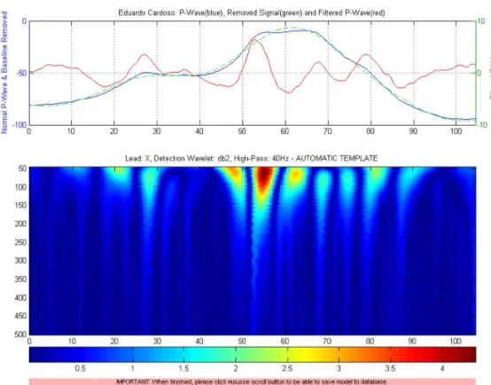
Figure 5.5– MicroECG obtained scalogram for the P-wave using the detection wavelet: db2………..…..pg.50
Figure 5.6– MicroECG obtained scalogram for the P-wave using the detection wavelet: fbsp1-1-1……….……pg.50
Figure 5.7– The original signal S, passes through two complementary filters and emerges as two signals……….….pg.51
Figure 5.8– The process on the right, which includes downsampling, produces DWT coefficients………..…pg.51
Figure 5.9– Wavelet decomposition tree………..……..pg.52
Figure 5.10 - Wavelet packet decomposition……….……pg.52
Figure 5.11– DWT reconstruction and respective values for the coefficients found for an eighth of the available frequency
band width. Only 32 of possible 256 coefficients are shown. The reconstruction of the signal, using all the found coefficients, when compared with the original signal suffers some degradation………pg.53
Figure 5.12– DWT reconstruction and respective values for the coefficients found for a quarter of the available frequency
band width. Only 64 of possible 256 coefficients are shown. The reconstruction of the signal, using all the found coefficients, when compared with the original signal suffers less degradation than the previous
example………pg.54
Figure 6.1 - ActiveTwo System and its components………pg.55
Figure 6.2 - Flat-type active-electrodes……….……...pg.56
Figure 6.3 - Analog/Digital Box………....pg.57
Figure 6.4 - USB2 receiver………..………pg.57
Figure 6.5 - ActiView software……….…….pg.58
Figure 6.6– Charger……….….pg.59
Figure 6.7 - Battery box………pg.59
Figure 6.8 - Analog Input Box………...pg.60
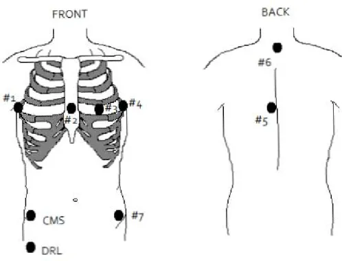
Figure 7.1 - Electrode positions used during the HR-ECG data acquisition (Frank’s leads)……….…..pg.62
Figure 8.1–MicroECG’s general process diagram……….…..pg.64
Figure 8.2–Late potential simulator diagram………..….pg.65
Figure 8.3–Open file diagram……….………….pg.66
Figure 8.4–Read file diagram………..pg.67
10
Figure 8.6–Show template diagram………..…..pg.70
Figure 8.7–Fine tuning diagram………..pg.70
Figure 8.8–ECG variability diagram………..pg.71
Figure 8.9–H.R.V diagram……….pg.72
Figure 8.10–Noise level diagram………pg.72
Figure 8.11–Raw data from electrodes diagram……….…….pg.73
Figure 8.12–12 Lead ECG diagram………...….pg.73
Figure 8.13–Magnitude vectors diagram………..……….pg.74
Figure 8.14–Wavelet diagram………..……pg.75
Figure 9.1 - Change "Current Directory"………..….pg.77
Figure 9.2 - MCRInstaller.exe is present in the given directory………..…pg.78
Figure 9.3 - .NET framework is not needed……….pg.79
Figure 9.4 - Click "Simulator" under the File tab………..….pg.79
Figure 9.5 - Late Potential Simulator………..………..pg.80
Figure 9.6 - Default beat detection values……….……….pg.80
Figure 9.7–"Automatic” Template……….………pg.82
Figure 9.8 - Show Template (delineated signal)………pg.82
Figure 9.9 - Fine Tuning……….…..pg.83
Figure 9.10 - "One Beat Correlation" method……….………pg.83
Figure 9.11 - "K Beats Average" method……….…….pg.84
Figure 9.12 - Open a real acquired signal……….…pg.84
Figure 9.13 - Recent recordings………...pg.85
Figure 9.14 - Personal Data, Recording Features………..……pg.85
Figure 9.15 - Previous recordings………..…..pg.86
Figure 9.16 - Reading .mat files………..…….pg.87
Figure 9.17 - Read File group box………..…..pg.87
Figure 9.18–Frank’s derivations (Vx, Vy and Vz)……….pg.88
Figure 9.19 - Scrolling and zooming through the data………...pg.88
Figure 9.20 - Heart Rate Variation………..……pg.90
Figure 9.21 - Raw Data from Electrodes………..……….pg.90
Figure 9.22 - Level Noise between Heart Beats (FFT analysis)……….………..pg.91
Figure 9.23 - Twelve Lead ECG………...…..pg.92
11
Figure 9.25 - ECG Variability (QRS Complex + T Wave / Selected Beats)………..…pg.94
Figure 9.26 - ECG Variability (QRS Complex + T Wave / All Beats) [Extra-systoles visible]………..……….pg.94
Figure 9.27 - Automatic Template Scenario………...pg.95
Figure 9.28 - Template's Title………pg.96
Figure 9.29 - Zoom and Restore Default Viewing……….…pg.96
Figure 9.30 - Zoomed in templates……….…pg.97
Figure 9.31 - Magnitude Vectors………pg.98
Figure 9.32 - Magnitude Vectors (P-Wave and QRS Complex)………..…..pg.98
Figure 9.33 - Magnitude Vectors' Fine Tuning………..pg.99
Figure 9.34 - Magnitude Vectors' Results………..pg.99
Figure 9.35 - Wavelet's interface……….………..pg.100
Figure 9.36 - Wavelet Scalogram (default values)………..………..pg.100
Figure 9.37 - Three wavelet scalogram (P-Wave, QRS Complex and T-Wave)……….pg.101
Figure 9.38 - Difference in both scalograms, the right one has a Threshold value of 0.3. The left one has no
Threshold………...pg.101
Figure 9.39 - Wavelet scalogram shows the difference between a filtered signal and a non-filtered signal…………...pg.101
Figure 9.40 - Wavelet scalogram showing the exact same signal, with all the same parameters in different
scales………..…...pg.102
Figure 9.41 - Normalization of a wavelet scalogram. From left to right the normalization suffered is 0, 0.5 and
1……….pg.103
Figure 9.42 - Simulated Late Potential (50:1:300)………..pg.103
Figure 9.43 – Different scalogram of a late Potential on an acquired signal. Frequencies used: 1:1:300 and
50:1:300………..………pg.104
Figure 9.44 - Selecting an artifact………..…..pg.104
Figure 9.45 - Nodes and corresponding values of a discrete wavelet transformation of the selected artifact………pg.105
Figure 9.46 - Save Model……….….pg.106
Figure 9.47 - Accessing the "Save Raw Data" feature………..………pg.107
Figure 10.1 - Magnitude vectors for both the P-Wave and the QRS Complex of a healthy subject……….…pg.110
Figure 10.2 - Statistical analysis (anoval1) for the values of P-Wave RMS20, 30 and 40 (µV). This procedure could not
differentiate any of these three parameters……….……….pg.111
Figure 10.3 - Heart rate variation on a healthy subject……….pg.112
Figure 10.4 - Heart rate variation on a subject that has cardiac extra-systoles……….pg.113
Figure 10.5 - Heart rate variation from a subject suffering from atrial fibrillation………pg.114
Figure 10.6 - Normal P-wave variability………..……pg.116
Figure 10.7 - Normal QRS complex variability………....……pg.116
12
Figure 10.9 - Heart Beat Variability (P-wave disappearance)………....pg.117
Figure 10.10 - Heart Beat Variability (P-wave disappearance - top view)……….………pg.118
Figure 10.11 - Heart beat variability (presence of seven extra-systoles)……….….pg.118
Figure 10.12– Wavelet scalogram on a healthy individual. Detection wavelet used is cmor1-1.5………pg.119
Figure 10.13– Scalogram showing a simulated late potential using the detection wavelet cmor1-1.5………..……..pg.120
Figure 10.14– Scalogram showing a simulated late potential using the detection wavelet fbsp1-1-1………..……pg.120
Figure 10.15–Scalogram from an acquired signal showing late potential………..……..pg.121
Figure 10.16– MicroECG allows zooming in on the late potential artifact………..…pg.121
Figure 10.17– MicroECG allows the user to extract the coefficients that constitute the late potential artifact….……...pg.122
Figure 10.18– MicroECG also presents the user a chart containing the RMS and power values of these
coefficients………pg.122
Figure 10.19 – Wavelet packet coefficients from 12 subjects lined side by side, allows seeing the ones suffering from atrial
13
Chapter 1: Objectives
Objectives
One of the major objectives of the development of this software package is that the MicroECG software could be used as a platform for future studies in cardiac signal processing. To do this the software package had to be as versatile and flexible as possible, regarding the cardiac arrhythmia.
The MicroECG software package contains the following features:
Versatile peak detection with wavelets and classical methods
ECG delineation using wavelet methods
Time-frequency analysis through scalogram
Spectral analysis using wavelet packet methodology
Selective reconstruction of the signal in specified frequency bands
Late potential detection using Simson’s method
Heart rate variation
ECG morphology variability
12-lead ECG display
14
Chapter 2: Introduction
2.1 Anatomy
The heart could be described as being 2 pumps. 1 pump (right side) sends blood to your lungs to be oxygenated and to remove waste products (CO2) and the other pump (left side) sends the blood around the systemic circulation to oxygenate all the cells in the body. The heart weighs between 7 and 15 ounces (200 to 425 grams) and is a little larger than the size of your fist; it is located between your lungs in the middle of your chest, behind and slightly to the left of your breastbone (sternum).
The heart has 4 chambers. Two upper chambers are called the left and right atria, and the two lower chambers are called the left and right ventricles. The septum (a wall of muscle) separates the left and right atria and the left and right ventricles. The left ventricle is known as the largest and strongest chamber in your heart with enough force to push blood through the aortic valve and into your body.
The heart chambers have valves which assist in the transport of blood flow through the heart, these are:
The tricuspid valve regulates blood flow between the right atrium and right ventricle.
The pulmonary valve controls blood flow from the right ventricle into the pulmonary arteries, which carry deoxygenated blood to your lungs to oxygenate.
The mitral or bicuspid valve lets oxygenated blood from your lungs pass from the left atrium into the left ventricle.
15
Figure 2.1 - Heart's blood flow. Extracted from http://www.ambulancetechnicianstudy.co.uk/card.html
2.2 Electrocardiography
In this chapter will be present the fundamental notions of the electrocardiographic genesis focusing the issue in the high-resolution electrocardiography (HR-ECG). Some of the major characteristics of the cardiac tissue will be explained as well.
The heart is a muscle made of four major parts; two atrial and two ventricular. The left and right ventricles push the blood to the pulmonary system and in the systemic blood circulation. Each heart beat is a mechanical process ruled by bioelectric phenomenon. The excitability and conductivity are essential properties of the cardiac tissues. These properties vary in their location inside the myocardial tissues. In periods of activity (systoles) or in periods of rest (diastoles) these cardiac cells are subjected to a series of complex electrical events on membrane or in intracellular space. These events have the primary function to promote the fast transmission of electrical impulses throughout the heart. This electrical activity verification is made through an electrocardiograph (ECG).
2.3 The heart dynamics
The right and left sides of the heart work together. Firstly, on the right side of the heart the blood enters the heart through two large veins, the inferior and superior vena cava, emptying oxygen-poor blood from the body into the right atrium. The same time, on the left side the pulmonary vein empties
oxygen-rich blood, from the lungs into the left atrium. Figure 2.2 - Blood
entering the heart. Right pulmonary
veins
Right atrium---t~~\
Inferior vena cava
Right ventricle
} Left pulmonary arteries
16
Then the atrial contraction takes place. On the right side of the heart the blood flows from the right atrium into the right ventricle through the open tricuspid valve. When the ventricles are full, the tricuspid valve shuts. This prevents blood from flowing backward into the atria while the ventricles contract
(squeeze). On the left side the blood flows from the left atrium into the left ventricle through the open mitral valve. When the ventricles are full, the mitral valve shuts. This prevents blood from flowing backward into the atria while the ventricles contract (squeeze).
The final movement is the ventricular contraction. Again, on the right side the blood leaves the heart through the pulmonic valve, into the pulmonary artery and to the lungs. As for the left side the blood leaves the heart through the aortic valve, into the aorta and to the body.
This pattern is repeated over and over, causing blood to flow continuously to the heart, lungs and body.
2.4 Depolarization sequence
The nerve fibers in their rest condition have fewer number of sodium ions in their inside that in their outside. This causes an electric tension between the inside and the outside of about 80 to 85 microvolts in the cardiac muscle. After an initial signal, a rapid diffusion of ions occurs on the inside in a short period of time. This causes a depolarization and inverts the potential. Shortly after, the sodium ions leave the inside and the membrane is polarized again. This polarization time is known as refractory period, in which the membrane cannot be depolarized again.
If a depolarization is ignited in a point, it will draw out through the membrane, causing a muscular contraction, with a speed of about 0.3 to 0.4 m/s to the auricular and ventricular fibers and till 100 m/s in larger nervous fibers. The refractory period in which the cardiac muscle cannot be excited is about 0.25 seconds and is known as functional refractory period. Still there is another relative refractory period that lasts about 0.05 seconds in which is hard, but not impossible to excite the muscle.
In the right atrium is a small section of specialized muscle called Sino-auricular nodule that has a low rest potential of about 55 to 60 microvolts and a constant escape of ions. This event causes a periodic auto-excitation. So each time the rest potential is set, the escape of ions causes a decrease of potential until the bottom limit is reached in the excitation phase. When this happens, Figure 2.3 - Atrial
contraction.
Figure 2.4 - Ventricular contraction.
Figures extracted from
http://my.clevelandclini c.org/heart/heartworks/
17
the Sino-auricular nodule will depolarize. This depolarization will be transmitted to both sides of the auricular muscle as it contracts with a 0.3 m/s velocity. As this impulse dislocates through the auricular muscle, it contracts. Given this transmission velocity the ventricular contraction would
happen before the ventricles are full of blood, so there is a delay mechanism. The
auricular signal reaches, in 0.04 seconds, to the Auricular-Ventricular nodule, located in the right atrium, being channelized to the Purkinje fibers, through the bundle of His. These high-velocity fibers conduct the signal to both ventricles in 2 m/s approximately, where then diminish to a 0.3 m/s.
2.5 Electrical System
The electrical system in your heart controls the speed of your heartbeat. Your heart has three main components to the system, these consist of:
S-A node (sino-atrial node) A-V node (Atrio-ventricular node) Purkinje system
The S-A node also called the "natural pacemaker", of your heart because it controls your heart rate. The S-A node is made of specialized cells located in the right atrium of the heart. The S-A node creates the electricity that makes your heart beat. The S-A node normally produces 60-100 electrical signals per minute — this is your heart rate.
The A-V node is a bundle of cells between the atria and ventricles. The electrical signals generated by the S-A node are "caught" and held for milliseconds before being sent onto the bundle of HIS (HIS Purkinje system).
Figure 2.6 - Heart's electrical system. Extracted from
http://www.ambulancetechnicianstudy.co.uk/card.html
Figure 2.5 - Human heart in detail. Extracted from
http://www.emergencymedicaled.com/215AED.htm SinO,Jtn,J1
(SA I
Righi Bundl. Bronch(RBBI
Right Ventricle
RighIB1IIIIIlo~""",h
Left Atrium
l'urkiJlje fib.", IPFl
18
HIS-Purkinje system is in your heart's ventricles. Electricity travels through the His-Purkinje system to make your ventricles contract. The electricity from the A-V node hits the bundle of HIS before being directed into the right and left bundle branches and finally into the Purkinje fibers that are located in the cardiac muscle. This stimulates the ventricles to contract.
2.5.1 Electrical Pathway
1. The S-A node creates an electrical signal
2. The electrical signal follows natural electrical pathways through both atria. The movement of electricity stimulates the atria to contract, which pushes blood into the ventricles.
3. The electrical signal reaches the A-V node. There, the signal pauses to give the ventricles time to fill with blood
4. The electrical signal spreads through the His-Purkinje system. The movement of electricity causes the ventricles to contract and push blood out to your lungs and body.
The name for the steps above is known as the cardiac cycle which lasts for 0.8 seconds:
Atrial systole = 0.1 second
Ventricular systole = 0.3 seconds
Diastole = 0.4 seconds
(Systole refers to the contraction of the cardiac muscle; Diastole refers to the relaxation of the cardiac muscle)
2.6 Nervous Control of the Heart
Although the S-A node sets the basic rhythm of the heart, the rate and strength of its beating can be modified by two auxiliary control centers located in the medulla oblongata of the brain.
One sends nerve impulses down accelerator nerves.
19
2.6.1 Accelerator Nerves
The accelerator nerves are part of the sympathetic branch of the autonomic nervous system. They increase the rate and strength of the heartbeat and thus increase the flow of blood. Their activation usually arises from some stress such as fear or exertion. The heartbeat may increase to 180 beats per minute. The strength of contraction increases as well so the amount of blood pumped may increase to as much as 25-30 liters/minute.
2.6.2 Vagus Nerve
The Vagus nerves are part of the parasympathetic branch of the autonomic nervous system. They, too, run from the medulla oblongata to the heart. Their activity slows the heartbeat. Pressure receptors in the aorta and carotid arteries send impulses to the medulla which relays these impulses back by way of the Vagus nerves to the heart. Heartbeat and blood pressure diminish.
2.7 Electric signals and electrocardiography
One electric fiber in depolarization may be compare to a current dipole. On a given instant, the activation wave’s front formed by elementary dipoles
creates an electric field in result of the dipolar moments. The time evolution registry of the electrical field is made through coetaneous electrodes is called electrocardiogram.
Electrocardiography is about 100 years old and coincides with the creation of the first registry system sensitive enough to measure the cardiac electrical potentials from the surface of the body. This system was first developed in 1903 by the Dutch Doctor Willem Einthoven [Einthoven, 1903]. He was awarded the Nobel Prize of Medical or Physiological Achievements in 1924.
2.7.1 Standard ECG acquisition: the derivations
A derivations system, in electrocardiography, consists in a coherent set of electrode locations, each one defined by their positions on the patient’s thorax. The positioning of the
electrodes is chosen on a way to cover the cardiac electrical potential through a set of non-redundant derivations. There are several standard systems. Now will be explained the most used systems in chronological order and what kind of electrocardiograms they are most associated.
Figure 2.7 - Willem Einthoven (1906). Extracted from
http://pt.wikipedia.or g/wiki/Willem_Eintho
20
Frontal plane bipolar derivations
The bipolar derivations DI, DII and DIII explore the cardiac activity in a frontal plane. This referential system is limited by an equilateral triangle (Einthoven Triangle). The three electrodes are placed respectively in the right arm (RA), on the left arm (LA) and on the left leg (LL). It is considered to all vectors to be instantaneous and have a common origin in the triangle’s center
and is projections are obtained through its sides, measuring the electric tension between the points:
𝐷𝐼 =𝑉LA−VRA (2.1)
𝐷𝐼𝐼 =𝑉LL −VRA (2.2)
𝐷𝐼𝐼𝐼 =𝑉LL−VLA (2.3)
And have the relation:
𝐷𝐼+𝐷𝐼𝐼𝐼 =𝐷𝐼𝐼 (2.4)
Frontal plane unipolar derivations
In 1934, Wilson introduced the unipolar derivations. [Kossman 1985] In this case the electric tension is measured between a point of reference and each one of the R, L, and F points. In this system the referential point is designed by
“Wilson’s Central Electrode” which is a virtual point and
supposedly has a null differential potential.
Goldberger [Goldberger 1942] proposed in 1942, the extended unipolar derivations (aVr, aVl and aVf). These derivations allow the acquisition of greater amplitude signals then the Wilson method. These derivations measure the
potential difference between each one of the three (RA, LA and LL) points and the mean potential from the other two. This way the electric tension is increased in a factor of 1.5 in comparison to the
Wilson’s derivations.
Figure 2.8 - Front plane bipolar derivations
Figure 2.9 - Frontal plane unipolar derivations. Figures extracted from Biomedical Digital Signal Processing,
Tompkins, pg.38 [Tompkins 1993]
DI
DII
Dill
_VA
aVL
21
𝑎𝑉𝑟=𝑉𝑅𝐴−𝑉𝐿𝐴−𝑉𝐿𝐿2 (2.5)
𝑎𝑉𝑙= 𝑉𝐿𝐴−𝑉𝐿𝐿−𝑉𝑅𝐴
2 (2.6)
𝑎𝑉𝑓=𝑉𝐿𝐿−𝑉𝑅𝐴−𝑉𝐿𝐴
2 (2.7)
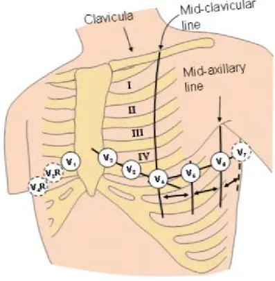
In 1935 Kossman proposed the unipolar thorax derivations (v1 to v6). These six unipolar
derivations run the precordial region and the left lateral transversally. They correspond to the
electric tension between each electrode and the “Wilson’s Central Electrode”.
Figure 2.10 - Electrode positioning in the unipolar derivations of the thorax (V1 to V6). Extracted from
http://www.bem.fi/book/15/15.htm [Malmivuo 1995]
C!CNlcuia
\
22
2.7.2 Formation of the ECG signal
The cells that constitute the ventricular myocardium are coupled together by gap junctions who, for the normal healthy heart, have a low resistance. As a consequence, activity in one cell is readily propagated to neighboring cells. It is said that the heart behaves as a syncytium; a propagating wave once initiated continues to propagate uniformly into the region that is still at rest.
Much of the knowledge about the activation sequence in the heart comes from canine studies. The earliest comprehensive study in this area was performed by Scher and Young. [Scher 1957] More recently, such studies were performed on the human heart, and a seminal paper describing the results was published by Durrer [Durrer 1970]. These studies show that activation wave fronts proceed relatively uniformly, from endocardium to epicardium and from apex to base.
23
,<IRIAL DEPOLAAII,<IION
00 . ,
SEPTAL DEPOLARIIATION
220m,
j
.00
Leod I
,apICAL DEPOLARII,<IION
230m,
LEfTVENTRICUL AA DEPOLAAII,<IION
24
Figures 2.11 – Sequence of the generation of the ECG signal in the Einthoven limb leads. Figures extracted from
http://www.bem.fi/book/15/15.htm [Malmivuo 1995]
LATE LEFT VENTRICULM DEPOLMIZATION
250 ms
VENTRICLES DE POLARIZED
350 ms
ri)
,,,
....
J
'....-...; :
'"~ .... _ - --
R"
P
JJ_
Q
~s
R
600 Ims] 400
Q
200
p
VE NTRICULAR REPOLMIZATION
450ms
VENTRICLES REPOLARIZED
600ms
T R
T
T
Q
25
After a while the depolarization front has propagated through the wall of the right ventricle; when it first arrives at the epicardial surface of the right-ventricular free wall, the event is called
breakthrough. Because the left ventricular wall is thicker, activation of the left ventricular free wall continues even after depolarization of a large part of the right ventricle. Because there are no compensating electric forces on the right, the resultant vector reaches its maximum in this phase, and it points leftward. The depolarization front continues propagation along the left ventricular wall toward the back. Because its surface area now continuously decreases, the magnitude of the resultant vector also decreases until the whole ventricular muscle is depolarized. The last to depolarize are basal regions of both left and right ventricles. Because there is no longer a propagating activation front, there is no signal either.
Ventricular repolarization begins from the outer side of the ventricles and the repolarization front "propagates" inward. This seems paradoxical, but even though the epicardium is the last to depolarize, its action potential durations are relatively short, and it is the first to recover. Although recovery of one cell does not propagate to neighboring cells, one notices that recovery generally does move from the epicardium toward the endocardium. The inward spread of the repolarization front generates a signal with the same sign as the outward depolarization front. Because of the diffuse form of the repolarization, the amplitude of the signal is much smaller than that of the depolarization wave and it lasts longer.
The normal electrocardiogram is illustrated in figure 2.12. The figure also includes definitions for various segments and intervals in the ECG. The deflections in this signal are denoted in alphabetic order starting with the letter P, which represents atrial depolarization. The ventricular depolarization causes the QRS complex, and repolarization is responsible for the T-wave. Atrial repolarization occurs during the QRS complex and produces such low signal amplitude that it cannot be seen
apart from the normal ECG. Figure 2.12 - The normal electrocardiogram. Extracted from
http://www.bem.fi/book/15/15.htm [Malmivuo 1995]
~ f- 5mm-...
It I
0.2 sec 5 mml
R 0.5 mV
H
II I !
1 mm 0.04 sec I~ 1 mm 0.1 mV
25 mmlsec 10 mmlmV)
p P-R '-f-8-T 4 T
....~ mentseg- segment ,/
1\
u--
/ !"I. 1/ 1\'"'"'"
r"I
-~
t-- P-R 1--1 Q interval
8-T
S in1terval
OR8 inte rval
O-T interval
26
2.7.3 Vectorcardiography
It was still in 1914 that Williams first came up with the concept of Vectorcardiography. Williams [Williams 1914] proposed a representation of the cardiac signal in four dimensions, time and space in three dimensions, comprehending the frontal sagittal, and transverse plane of the human body, as seen on figures 2.13. Vectorcardiography is based on the theory of the unique dipole through which all information about the cardiac activity manifests, on a given instant, through the form of an electric field vector with the origin, on the 0 point, which represents the electric center of the ventricular mass. This 0 point is fixed and is utilized as the point of origin of all resulting instantaneous vectors that evolve through time.
Figure 2.13 - The projections of the lead vectors of the 12-lead ECG system in three orthogonal planes when one assumes the volume conductor to be spherical homogeneous and the cardiac source centrally located. Extracted
from http://www.bem.fi/book/15/15.htm [Malmivuo 1995]
Each sequence of the cardiac electric field, P, QRS and T may be represented by a set of successive of resulting vectors and constitute a spatial curve named vectorcardiogram.
Frank, in 1956, utilized a system of derivations in X, Y and Z with clinical applications and it is still today, one of the most used vectorcardiographic systems. [Frank 1956]
v,
SAGITTAL PLANE
y
FRONTAL PLANE
v,
V,
27
It was this vectorcardiographic system used in the data recording sessions to obtain the
three Frank’s derivations because of his correct orthogonal system since allows to see the changes in morphology in a spatial orientation.
All three Frank’s derivations are obtained through a network of resistors that linearly
combine all potentials obtained through eight coetaneous electrodes, as seen on figure 2.14.
This system must still be normalized. Therefore, resistors 13.3R and 7.15R are connected between the leads of the x- and y-components to attenuate these signals to the same level as the z-lead signal. Now the Frank z-lead system is orthogonal.
It should be noted once again that the resistance of the resistor network connected to each lead pair is unity. This choice results in a balanced load and increases the common mode rejection ratio of the system. The absolute value of the lead matrix resistances may be determined once the value of R is specified. For this factor Frank recommended that it should be at least 25kΩ, and preferably 100 kΩ. Nowadays the lead signals are usually detected with a high-impedance preamplifier, and the lead matrix function is performed by operational amplifiers or digitally thereafter. Figure 14 illustrates the complete Frank lead matrix.
It is worth mentioning that the Frank system is presently the most common of all clinical VCG systems throughout the world. (However, VCG's represent less than 5% of the electrocardiograms.).
Figure 2.14 - The lead matrix of the Frank VCG-system. The electrodes are marked I, E, C, A, M, F, and H, and their anatomical positions are shown. The resistor matrix results in the establishment of normalized x-, y-, and z
-component lead vectors, as described in the text.
R III(;HT
H
•
•
1I
".27R•
V
z"
"
a.32ft. LEI'T+
E
"
3.74RE C
.-C
FItO~T_
•
A
~V,
0
+
1./8R
flACK
M
2.90R.",'"
I.53ft +
F
F
V~
•
RH
Jo ....\ •
28
The referential system is a tri-orthogonal rearrange where all axes are adapted to the geometry of the thorax; OX transverse, OY frontal and OZ sagittal. The signals registered in X, Y and Z is the projections of the instantaneous vectors over all three axes. This way Vx, Vy and Vz are given
by:
𝑉𝑋= 0.61𝑉𝐴+ 0.171𝑉𝐶−0.781𝑉𝐼 (2.8)
𝑉𝑌 = 0.655𝑉𝐹+ 0.345𝑉𝑀−1𝑉𝐻 (2.9)
𝑉𝑍 = 0.133𝑉𝐴+ 0.736𝑉𝑀−0.264𝑉𝐼−0.374𝑉𝐸−0.231𝑉𝐶 (2.10)
These equations are used in the developed software package to transform the obtained VCG
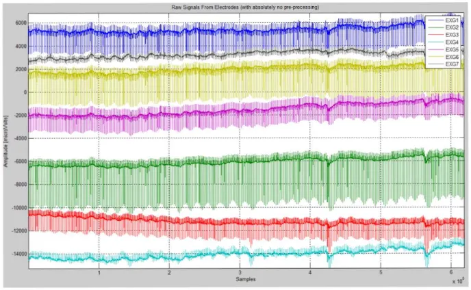
signal into the three Frank’s derivations. As seen from figure 2.15 the seven channels obtained , in MicroECG, through the VCG recording sessions are inputs for these equations. The result can be seen on figure 2.16 as the three Frank’s derivations are obtained by MicroECG.
Figure 2.15 – The seven electrode channels obtained through Biosemi’s ActiveTwo acquisition system using the
Frank’s lead VCG system.
I
,
1
"
RawSIgnals From Ele<:j,cxles (W1tn absolutely no pre-Jlfocessing)
J
29
Figure 2.16 –The three Frank’s derivations (Vx, Vy and Vz) obtained in MicroECG by using the seven electrode
channels as input of the Frank’s VCG equation system. (Equations 2.8, 2.9 and 2.10)
2.8 High-resolution electrocardiogram (HR -ECG)
High-resolution electrocardiography is considered to be a recent technique that only in 1972 was described for the first time in terms of signal analysis. [Evanich 1972] The high-resolution ECG is a method that allows increasing the signal/noise relation of the electrocardiogram. This method is largely used to register the transitory cardiac signals with low amplitude and high frequency, impossible to detect on a classic electrocardiogram. The utilization of the signal averaging is a method that supports on the fact of the electrocardiographic signal repeats itself on each cardiac cycle. By making the average over the number of N cycles (N [50,300]), allows to reduce quite
significantly the noise in a 1/ 𝑁 reason, with the conservation of the information that are synchronous in each cycle.
:g
1000~
I
500-500
2000
;gr 1500
i
1000.
"
:§ 500
~
<
:g
1000~
I
5001)\
1)\
;
'Ix~ime (8)]
- '
A A,
lfi
,
c , ,
;
Vi~ime (8)]
1\1
V
1\1
'\I
c , ,
;
30
The calculation of the ECG average needs a pre-treatment to detect and align the successive heart beats.
The quality of the electrocardiographic registry is dependent of the acquisition system, from the sampling frequency and from the presence of electrical and magnetic interferences. The electrical interference of muscular origin is a very important component of the interference and it is very hard to eliminate.
The presence of interferences induces a fundamental problem in high-resolution-electrocardiography because the noise is constituted by low amplitude, high frequency signals, much as the late potentials that appears on post-stroke patients or with tachycardia problems. For the needed precision, the technical characteristics of classical registry systems (gain, amplitude resolution, sampling frequency, etc) are general case, insufficient.
A possible application of the HR-ECG it is his utilization on the detection of late potentials on patients that suffered myocardium infraction. [Gomes 1972] On the late 1970’s, a common and growing interest on the comprehension of the mechanisms that generate ventricular arrhythmias conduct to the study of abnormal mechanisms on the ventricular depolarization, specifically on the QRS complex. The most notable study that still holds as a reference to this domain is the work of Simson that showed the relation between the presences of late potentials and the risk of ventricular tachycardia. On the sequence of Simson’s work, many more followed, however the methods of
acquisition and pre-treatment were so diversified that all the results became practically impossible to compare. So in order to standardize this method an international consensus was created, suggesting some norms over the acquisition techniques and processing of the HR-ECG data. [Breithardt 1991]
2.8.1 HR-ECG acquisition
The first generation of high-resolution electrocardiographic devices was limited to analog acquisition systems, however since 1979, digital acquisitions systems became present that allowed
to a, posterior, digital treatment of the results, that weren’t possible before.
31
Figure 2.17 - HR-ECG electrode positioning.
The quality of the skin/electrode interface should be optimum. Ag/AgC electrodes are normally used, since they are the most accurate for standard registration, however no study to date, verified this matter for the HR-ECG.
The gain in the amp of these acquisition system is normally fixed somewhere on 1000 to 8000 for frequencies comprehended on 0.5 to 300 Hz, but this value depends on the analog/digital
converter’s resolution.
2.8.2 Signal Averaging
After the amplification and analog filtering, the signal will be digitalized. The AD-Box was used with the following settings on the new recording sessions; a 2048 Hz sampling frequency and the amplitude of the signal was codified on a 24 bit with a 31nV resolution (LSB).
The detection of the QRS complexes (R points) should be made in three steps:
1. A IIR (Infinite Impulse Response) 1st order Butterworth filter is applied on a passing band between 5 and 30 Hz, to avoid tension fluctuations across the QRS complex and to eliminate DC components introduced by the skin/electrode interface e mainly because the largest part
of the energy of the QRS complex’s signal is found on the passing band referred.
2. An algorithm is applied, that detects relative maximum points over a given “threshold”
value, on the filtered signal.
3. Because filtering always causes a displacement of the signal, another algorithm to detect the relative maximum point of the original signal. This way the R point for each heart cycle is
32
After the detection step, the classification of the QRS complexes is essential part of the process, to exclude the noisy heart beats. In HR-ECG the selection of the QRS complexes is made through an algorithm that uses a value of correlation between the complex to analyze and a complex of reference. The recommended value to the coefficient is generally superior to 0.95.
The synchronization of the complexes is made through a function of correlation calculated between each QRS complex of a heart beat and a QRS complex of reference. This synchronization should apply to all the cardiac cycle and not just the QRS complex, because the study of the P wave is also important. The correlation coefficient is given by the equation:
𝜌
=
𝑀𝑖=1𝑥𝑖𝑦𝑖𝑀 𝑥𝑖2
𝑖=1 𝑀𝑖=1𝑦𝑖2
(2.11)
Where xi and yi are respectively the M values that constitute the signal of the reference cycle and the signal to align. A minimum value of correlation accepted was established on 0.97 in with is considered an acceptable synchronization. In practice and after the study of Lander, the value of this correlation was set between 0.95 and 0.99. [Lander 1992]
The reference cycle 𝑦 (𝑛) is given by:
𝑦 𝑛
=
𝑅𝑖=1𝑥𝑖(𝑛)𝑅 (2.12)
The calculation of the mean signal 𝑥 (𝑛) of R cycles is given by:
𝑥 𝑛
=
𝑅𝑖=1𝑥𝑖(𝑛)𝑅
=
𝑠𝑖(𝑛) 𝑅 𝑖=1
𝑅
+
𝑏𝑖(𝑛) 𝑅
𝑖=1
𝑅 (2.13)
Where 𝑥𝑖(𝑛) represents all the electrocardiographic signal and 𝑠𝑖(𝑛) and 𝑏𝑖(𝑛) are,
respectively, the useful signal and the signal’s noise of n points on the i cycle. The origin of n is found
relatively to a point of synchronization linked to the useful signal.
The signal/noise relation (RSR) is defined by the module of the signal over the noise’s power:
𝑅𝑆𝑅
=
𝑠(𝑛)𝜎𝑏(𝑛) (2.14)
Where 𝜎𝑏(𝑛) is the standard deviation of the noise’s value on n points. This signal/noise
33
𝑆𝑅
𝑅=
𝑅𝜎𝑅 𝑠(2𝑛()𝑛)=
𝑅 𝑠(𝑛)
𝑅𝜎𝑏(𝑛)
=
𝑅𝑆𝑅 𝑅
(2.15)The conclusion of this last equation is that the reduction of the noise is proportional to the square root of the number of cycles.
MicroECG uses these same signal averaging principles to reduce the noise in the signal. This signal averaging process will not only obtain a template signal of the systematic heart beat signal but will also decrease the template’s noise. This noise present in the acquired data, as seen on figure 2.18 is often attributed to internal factors such as muscular activity or to external factors such as environment electromagnetic noise. The signal’s template, as seen on figure 2.19, will be a “cleaner”
signal than a random heart beat selected from the acquired data.
Figure 2.18 – Noisy signals are often seen even in high quality equipment such as the one used, most of these noise are due internal factors such as muscular activity or external factors such as environment electromagnetic noise.
_Yi,uoitlzef
;gr 1000
0
~ ;CO
C
·
"
~
~
<
-500
2H.1 27U 27U 27(( 2H.5 2H.6 270 2H.8 27(9 m
'Ix~ime (8)]
2000
:g
1500~
C
1000·
" ;CO
~
~
<
, , , , , , , ,
2H.1 27U 27U 27(( 2H.5 2H.6 270 2H.8 27(9 m
Vi~ime (8)]
;gr 1000
0
~
C
'CO·
"~
~
<
, ,
2H.1 27U 27U 27(( 2H.5 2H.6 270 2H.8 27(9 m
VI[time(8)]
34
Figure 2.19 – A heart beat template is a smoother signal due to signal averaging.
The heart beat template is a smoother signal due signal averaging. As seen in the figure 2.19 the template uses around 280 of 300 beats found to perform this signal averaging. All the selected beats will be cut in the same sample size, aligned and an averaging of these beats will construct a smooth and much less noisy heart beats’ template signal.
Automatic Template (XVector) - Detected Beats: 215 of 300
Used method- Conventional @Correlation- 0 99
, , , ,
V
, , , ,2IJJ ::OJ 400 500 600
Time Ims]
Automatic Template ('fVector) - Detected Beats: 286 of 300
Used method: Conventional @Correlation: 0_99
2IJJ ::OJ 400 600
Time Ims]
Automatic Template (Z Vector) - Detected Beats: 285 of 300 Used method: Conventional @Correlation: 0_99
c---+~~-T--+
'"'
Time Ims]
,
35
Chapter 3: Cardiac Arrhythmias
3.1 Reentrant circuits
Arrhythmias could be generated by several distinct mechanisms, however the one most associated with the appearance of late potentials is the reentrant circuit mechanism. This is the most common mechanism and is due to the existence of unidirectional blockage of ways or paths in the heart that facilitate the start and maintenance of these mechanisms. The reentrant arrhythmias are generally induced by atrial or ventricular ectopic heart beats that could be ignited by excessive injection of caffeine or alcohol.
Figure 3.1 shows the electric flow as it reaches the A, B base and divides in two. On A the flow is detained by a non susceptible zone to depolarization. On B the flow heads for the C trench, only to propagate after to A again, on reverse, where originates a re-excitation of the heart tissues.
3.2 Late Potentials
Late potentials are scattered, low-amplitude and abnormal micro-potentials, (about 25 microvolts in amplitude) due to reentrant circuit activity. The first study to observe the presence of late potentials realized on a dog, after a myocardium infraction, was performed by Boineau and Cox. [Boineau 1973] Then a study by Williams showed that late potentials are markers of the presence of reentries capable of generate ventricular arrhythmia. Just in 1986, Kuchar [Kuchar 1986] demonstrated that only patients that conserve these late potentials several days after the myocardium infraction are suitable to suffer ventricular tachycardia or even sudden death.
So, cardiac late potentials are low amplitude signals that occur in the ventricles. Also called Ventricular Late Potentials (VLPs), these signals are caused by slow or delayed conduction of the cardiac activation sequence. Under certain abnormal conditions, there may be small regions of the ventricles within a diseased or ischemic region that generate such delayed conduction. This results in depolarization signals that prolong past the refractory period of surrounding tissues and re-excite the ventricles. This re-excitement is known as 'reentry'. Reentry is believed to be a key factor that causes VLPs.
Figure 3.1 - Circuit reentry. Extracted from Slama, "Aide mémoire de la rythmologie", pg. 26 [Slama 1987]
36
Due to their very low magnitudes, late potentials are not visible in a standard ECG. Moreover, factors such as increased distance of the body surface electrodes from the heart, and inherent noise in patients make identification of VLPs beyond the resolution limits of a standard ECG. As a result, high-resolution recording techniques and computerized ECG processing are necessary for detection of late potentials. Figure 3.2 shows an historical figure where the patients’
magnitude vector clearly shows VLPs on the QRS complex signal. ECG signal processing includes techniques to improve the signal-to-noise ratio (SNR). One widely used technique to improve the SNR of ECG signals for the detection of late potentials is signal averaging.
Figure 3.2 –Historical picture of a patient’s magnitude vector with positive late potentials on QRS Complex. Figure extracted from http://cogprints.org/4314/1/hrecg.htm
3.2.1 Ventricular Arrhythmia and late potentials
The most common application of the HRECG is to record very low level (~1.0-μV) signals that occur after the QRS complex but are not evident on the standard ECG. These “late potentials”
are generated from abnormal regions of the ventricles and have been strongly associated with the substrate responsible for a life-threatening rapid heart rate (ventricular tachycardia).
In the last years, the ventricular late potentials detection has been used to study the conduction disturbances in the cardiac ventricles. The ventricular late potentials are composed by high frequency and low amplitude signals that occur in the last portion of the QRS complex and/or in the
QRSD _ I.saO
RMS40 _ 4.51
LAS40 _ 85.0
POlcnli.ls
QRS
~
60 120 11'0 Z40 300 l60 410 480 5'0 600
O.U
o
",
66.11
160.00
U.))
4'.'7
40.00
]J.ll
7";.11
20.00
,U
p
I
13.ll37
beginning of the ST segment. It was postulated that these late potentials would constitute invasive markers of the presence of an arrhythmogenic subtract, characterized by a slow and non-homogeneous propagation of the intraventricular activation wave.
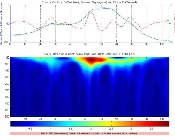
MicroECG does this magnitude vector study from the template obtained from signal averaging. As figure 3.3 shows the magnitude vectors are split in two charts; the upper green-delineated chart is corresponding to the P-wave magnitude vector as for the lower red-green-delineated chart corresponds for the QRS complex magnitude vector. Both charts are shown similarly to the historical figure 3.2 in µV / ms. As the historical figure 3.2 only shows only parameters corresponding to the QRS Complex, MicroECG is capable of studying both magnitude vectors because there are a series of parameters shown below the charts that correspond to the P-wave and the QRS complex.
Figure 3.3 –MicroECG’s studyfor the template’s magnitude vector for both the P-wave and the QRS complex. Shown are ventricular late potentials and their respective parameters values.
om
'"'
Vector Magnitude P - Time [miliseconds]
TIME DOMAIN (Automatic Template)
~ _ _~ _ _~-. _ _~C- _ _~':"-'--. ~-,
,
, , , ,
,
, , , ,
,
,
,
,
LAS40< :".'..,,,'44.1661 I
i
:Late Potentials
520 540 560 560
Vector Magnitude QRS - Time [miliseconds]
QRSComplex' ,
RMS30 uY 1.1259
Pw.... ,