A genetic algorithm to solve a multi-product distribution problem

(1)

A GENETIC ALGORITHM TO SOLVE A

MULTI-PRODUCT DISTRIBUTION PROBLEM

by

Bruno Miguel Ribeiro Crétu

Master in Data Analytics Dissertation

Supervised by:

Professor Dalila B. M. M. Fontes

Faculdade de Economia Universidade do Porto

(2)

i

Biographical Note

Bruno Miguel Ribeiro Crétu was born on the 12th of May 1994, in the city of Porto.

After finishing his bachelor in Business Administration at Porto School of Economics in 2015, he proceeded his studies with the Master in Data Analytics. During his bachelor, he became a member of a student organization, the Experience Upgrade Program, and was a summer intern at Frederico Mendes & Associados, a consulting firm.

While in his master he was admitted as an intern in Sonae’s SR fashion division MO, fulfilling the role of Business Analyst. As of April 2017, he left his position to dedicate his time to the master thesis and other personal projects.

Additionally, he practices sport, namely rowing, since he was 9 years old. During this period, he competed internationally, for his club and national team.

(3)

ii

Acknowledgements

First, I want to thank Professor Dalila for accepting this challenge and for her crucial help in building this thesis. Without her help, ideas and high spirits this wouldn’t be possible.

A big thanks to all my family and friends. They listened to my complaints and understood my absence of mind during this period. Even though no one understood what I was stressing about, they took the time to listen and calm me in a certain way. To the family specifically, thank you for teaching me perseverance and ambition, it was key on hard moments. To the friends, thank you for the company, the drinks, the conversations that kept my mind of problems when I most needed.

As a rower, rowing was also the perfect escape to either get my mind of things or to think about how to overcome the issues that I came across. Thank you to the big team of Sport Clube do Porto for creating the perfect training atmosphere, and of course to my teammates Tito, João and Guilherme.

Finally, but not least important, to all the people of online forums or websites that posted questions and answers to all kinds of problems. For a person who is learning, many questions came up, but none was left unanswered. I know you will never get to read this, but a big thank you!

(4)

iii

Resumo

Esta dissertação tem como objetivo criar uma ferramenta que apoie a tomada de decisão dos gestores de downstream de uma empresa de moda portuguesa. Os gestores devem decidir enviar determinados produtos de um armazém para cada uma das lojas e especificar as quantidades. Escolhemos abordar este problema duma perspetiva de minimização de custos, mas com especial interesse nas restrições.

Sendo um problema combinatório difícil, é necessário utilizar uma heurística. Como os Algoritmos Genéticos são conhecidos pela sua eficiência na resolução deste tipo de problemas, propomos construir um adequado ao problema a resolver. Os resultados mostram que o algoritmo é capaz de resolver o problema de forma eficiente, eficaz e, sobretudo, ser uma ferramenta de apoio à decisão.

Palavras chave: algoritmo genérico, gestor downstream, cadeia de abastecimento,

(5)

iv

Abstract

The dissertation aims at creating a tool to support the decision making of downstream managers of a portuguese fashion company. The managers must decide whether to send a certain product to each store, and specify the quantities, from one warehouse. We chose to approach the problem with a cost minimization perspective, but with special interest on the constraints.

Being a hard combinatorial problem, a heuristic had to be used. Since Genetic Algorithms have been known to be efficient at solving this kind of problems we propose to build one suited for it. The results will show that the algorithm is capable of solving the problem efficiently, effectively and, ultimately, being a decision support tool.

Keywords: genetic algorithm, downstream manager, supply chain, optimization,

(6)

v

1.1. Methodology ... 2 1.2. Context ... 3 1.3. Dissertation structure ... 6 2. Problem description ... 7 2.1. Detailed description... 8 2.2. Model formulation ... 11 3. Solution approach ... 15 3.1. Problem representation ... 17 3.2. Initial population ... 18 3.3. Fitness function ... 19 3.4. Genetic operators ... 23 3.4.1. Selection ... 24 3.4.2. Crossover ... 25 3.4.3. Mutants ... 27 3.4.4. Parameters ... 28 3.5. Repair function ... 31 4. Computational experiments ... 34 5. Conclusions ... 40 6. Bibliography ... 42 7. Appendix ... 45

(7)

vi 7.1. Appendix 1 ... 45 7.2. Appendix 2 ... 46 7.3. Appendix 3 ... 52 7.4. Appendix 4 ... 53 7.5. Appendix 5 ... 56 7.6. Appendix 6 ... 59 7.7. Appendix 7 ... 61

(8)

vii

List of Figures

Figure 1 - Product Structure. ... 4

Figure 2 - Problem representation example. ... 17

Figure 3 - Floating point chromosome example. ... 18

Figure 4 – Pseudocode: initial population. ... 19

Figure 5 – Pseudocode: awarding points regarding constraint (5). ... 21

Figure 8 – Pseudocode: awarding points regarding constraints (10) and (11). ... 22

Figure 10 – Pseudocode: awarding points regarding the cost score. ... 23

Figure 11 - New population example. ... 24

Figure 12 – Pseudocode: Elite function. ... 25

Figure 13 - 1-point crossover (left) and 2-point crossover (right) examples. ... 25

Figure 14 - 2-point crossover issue. ... 26

Figure 15 – Pseudocode: selection of parents and crossover. ... 27

Figure 16 – Pseudocode: Mutation.. ... 28

Figure 17- Comparison of two good performing tests with two underperforming tests. 31 Figure 18 – Pseudocode: warehouse inventory repair function. ... 32

Figure 19 – Pseudocode: store inventory repair function. ... 32

Figure 20 – Pseudocode:4 week sales repair function. ... 33

Figure 21 – Pseudocode: repair function (condition 4) ... 33

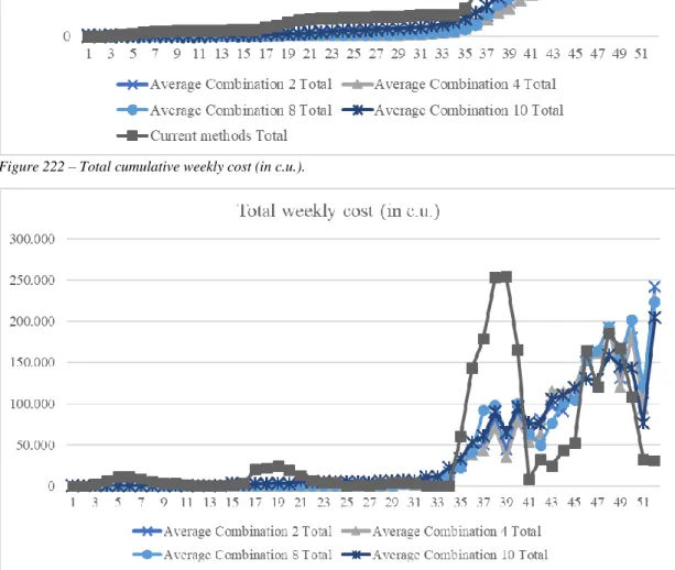
Figure 22 – Total cumulative weekly cost (in c.u.). ... 35

Figure 23 - Total weekly cost (in c.u.). ... 35

Figure 24 - Warehouse Hold Cost vs Store Hold Cost. ... 38

(9)

viii

List of Equations

Equation 1 - Days of coverage formula. ... 3 Equation 2 - Objective function and constraints. ... 13

(10)

ix

List of Tables

Table 1 - Notation ... 12

Table 2 - Score system details. ... 20

Table 3 - Combinations of the genetic operators’ parameters. ... 28

Table 4 - Population parameter values. ... 29

Table 5 - Generations Parameter. ... 29

Table 6 - Top four test results. ... 30

Table 7 - Test results, means and standard deviations. ... 37

(11)

1

1. Introduction

1.1. Objectives and motivation

The apparel and textile industry yields great importance to the European Union,

employing more than 1.6 million people, in 20151. Besides its importance to the job

market, it is responsible for dressing people around the world which affects cultural interactions and standards.

The increasing volatility, competitiveness and short product lifecycle requires an efficient response from the market players (Bruce, Daly, & Towers, 2004). Depending on the strategic orientation of each company (e.g., luxury vs fast fashion), seeking lower costs to achieve high return on margin is a priority for the companies. To accomplish this, companies resort to global sourcing, adopting an integrated system known as supply chain management.

The tool that we propose to solve is aimed at supporting the decision making process of managers that integrate the supply chain of a fashion company. We aim at creating a tool that will effectively and efficiently give the quantities, of each product, that the manager should send to each store of the company, at a minimum cost. However, as it will be explained, cost is not the only issue, so here we are also proposing a new point-of-view of how to manage the stocks. The company has one warehouse that is stocked every week. With the stock available in the warehouse, the managers need to find the best way to allocate it to each store. Therefore, the algorithm’s output will be the quantity of each product to be sent to each store, while minimizing the cost.

The problem addressed here belongs to the combinatorial class as it involves finding an assignment of a discrete finite set of objects, while satisfying a given set of conditions. In addition, realistic problem instances involve many objects and decisions. Therefore, the methodology to develop must be heuristic in nature. Amongst the many existing heuristics, genetic algorithms have been chosen, mainly due to:

1_Statista:

(12)

2

i. The good performance (runtime, feasible solutions ratio and solutions quality)

in many other combinatorial problems

ii. Mentor’s experience with these types of heuristics, which will ease the learning

process.

1.1. Methodology

We will use a genetic algorithm (GA) built from scratch in Python language. The programming language chosen is, first, the one that the mentee has some knowledge of and, secondly, Python’s flexibility, simple syntax and massive community make it a perfect language to learn in such a short span. Flexible, because there are no hard rules on how to build a script and problems can be approached through many methods. The code is read like English, focuses on concepts and avoids details. Across the top programming communities (e.g., GitHub, StackOverFlow, Meetup, etc.) the language is on the top in terms of members and projects. This allows an easier option to solve any kind to problem.

The algorithm is basic in its implementation and contains the following usual features of a GA:

• Randomly generated population where each store and product is represented; • Fitness function that computes the score of each individual solution not only

based on the cost but also on the compliance with the constraints;

• Elitism that transfers the top percentage of solutions into the next generation; • A crossover operator that pairs two chromosomes with an adaptation of the

1-point crossover and an elitist pool to select the parents;

• And finally the introduction of mutants instead of a mutation operator based on the biased random-key genetic algorithm (BRKGA) (Toso & Resende, 2015).

The code presented here was designed to answer to the problem described in the dissertation. However, with small changes to the code it may be adapted to similar problems, even if unrelated.

(13)

3

1.2. Context

To begin with, we need to understand the context where the supply chain is inserted, i.e., organizational structure and product structure. The problem that we tackle is based on a specific structure of a Portuguese Fashion Store. The information will not reveal any business specific aspects, the latter ones are omitted. Data deemed relevant, but impossible to bring to light, will be fictitious and properly stated in the assumptions.

Structurally speaking there are three main areas on the supply chain: Upstream, Downstream, and Quality Management. The tool being presented here is intended to be applied by the Downstream Manager (DM)

The DM’s job is to determine the optimal quantity of each product to be sent to each store while satisfying certain business parameters. The parameters include minimum and maximum amounts per product per store. These limits are adjusted over time, mainly as a consequence of problems that the stores communicate to the central offices or as strategic decisions.

Currently, the decisions of whether to send each product or not is heavily dependent on appropriated days of coverage (DC). There is a business reference to how many DC there should be. The company has a threshold of 4 weeks. The DC provides the information of how many days the current in-store stock can cover, given the value/quantity of sales, over a certain period of time, as given in the following equation.

𝐷𝐶𝑖 = (

𝑠_𝑖

∑𝑡_𝑗=𝑖𝑝_𝑗) × 𝑡 − 𝑖 + 1 Equation 1 - Days of coverage formula.

The days of coverage in period i (DCi) is calculated as the ratio of the stock in period

i (si) and the to be projected sales (p) from period i until period t, where t is the size of the

time window of analysis, usually the whole season (6 to 8 months).

However, currently, the sales used to obtain the coverage days are last year’s sales plus a growth rate, based on the previous two weeks uplift. Using the previous year sales data as a decision factor to supply the stores raises the crucial issue: strategy. In other words, an apparel collection is built based on the homologous period (i.e., Autumn/Winter’17 is

(14)

4

based on Autumn/Winter’16), but the merchandiser2_{takes strategic decisions, not only to}

amend past failures but also to react to trends.

Consider the following example of how it impacts the DM’s job: if the merchandiser plans to buy more shirts because the market points in that direction. The result of the DM’s analysis will be high (unusual) DCs. The increased purchase of such items leads to an inventory that is larger than required to cover the last year’s sales. If the DM is not aware of the strategic decision, he/she can make the decision of not sending more shirts so that stores are not overburdened with stock. The reverse may also happen. The DM might detect that there is not enough stock to supply all the stores. When the merchandiser proposedly bought less of that product to make up for waging on other products.

To overcome this, a budget that reflects the strategy of each type of product (e.g., T-shirts) is necessary. The DM needs to review the given initial budget, every week, alongside with a markets team to properly address outliers that are not obvious in the initial build of the budget. Or if any major changes are made to the promotional activities (i.e., discounts or store events).

The collection is split into two major groups that require different treatment. On the one hand, we have the seasonal collection. It changes according to the season and is rarely repeated after one season. On the other hand, there are items that are permanently in-store, which are known as the never out of stock products (NoS). They require a type of management different than that of the seasonal items.

The product structure is straightforward:

2_{Person responsible for planning the collection, who selects which products will be in-store, price and}

promotional highlight.

(15)

5

The category is the most macro point-of-view one can have at the company. At this level, there are eight (8) categories, four for woman and four for man, as follows: Apparel, Underwear/Nightwear, Footwear and Accessories. The Woman and Man Apparel are the main categories so each requires a DM. The other categories have one manager per gender (i.e., a DM for Underwear/Nightwear, Footwear, and Accessories for Man and another for Woman).

The subcategories aggregate the collection into segments. The aggregator is particularly important on the apparel and underwear/nightwear categories. The apparel subcategories correspond to brands (e.g., Casual Collection, Teen Collection and Basics Collection), while the underwear/nightwear are more specific groups (e.g., Nightwear, Underwear, Lingerie, Slippers, Socks).

The base unit identifies the type of product of each sub-category. One base unit can have multiple styles but it belongs to one subcategory only, examples of a base unit can be T-shirts or Outerwear.

The two most detailed levels are the Style and SKU. The Style is a specific product/color, so a red T-shirt and a green T-shirt are by default categorized under different styles each. There is never the same code season after season. Whereas, the SKU is the size of a given Style.

The supply is mainly done in packs of products. The packs have a set of sizes (e.g. one pack may contain 1 unit of size S, 2 of size M, 2 of size L, and 1 of size XL) and are used to do the first supply of the store. It represents 60-80% of the purchase done. Each store has a minimum pack required (associated with its sales and sales space capacity). If the sales are higher than expected, the downstream manager can re-supply using the “color-size”. The “color-size” are specific sizes of a style (e.g., red T-shirt of size M).

Due to the data availability, we can only approach the problem from a category point of view. Thus, we will work with 8 products - Apparel, Underwear/Nightwear, Footwear and Accessories for both Man and Woman. Henceforth, when we refer to “product” we are talking about a specific category.

(16)

6

1.3. Dissertation structure

We will start by defining the problem in Chapter 2, which includes a detailed description of the problem, assumptions, variables, and the mathematical formulation. Chapter 3 will dive into the approach taken in solving the problem, and describe the construction of the algorithm. In Chapter 4, we will discuss the computational experiments and results with the methodology that is currently adopted. Finally, Chapter 5 will summarize the conclusions of the work developed and suggest further work and improvements.

(17)

7

2. Problem description

The problem to be solved in the dissertation fits, in most part, in the Lot Sizing Problem (LSP). However, as we will see, it includes characteristics of multiple variants of the latter one. The LSP has many variants resulting from the introduction of new issues to better describe the problem that each author wanted to tackle. Over time several extensions have been considered, such as, limited capacity of both production and storage (Rogers, 1958); Hanssmann, 1962, production of multiple items (Elmaghraby, 1978; Hsu, 1983; Du Merle, Goffin, Trouiller, & Vial, 2000) and backlogging (Zangwill, 1969). The combination of the modifications over time lead to the economic lot scheduling problem, which in addition to finding the production amount for each product one also wants to find out which product is to be produced and when.

In short, the LSP consists of determining the production quantities for a specific time horizon, on a single or multi-level, for a specific number of products. There are capacity and/or resource constraints, and it need to satisfy a known or unknown demand at a minimum cost while maximizing the service level.

This dissertation focuses on a specific context and uses a genetic algorithm to solve it. Nevertheless, it takes into consideration the inputs of several authors that already explored the problem, even if in different contexts. As we will see, the problem has been tackled from an industrial point of view, so for example, variables such as set up costs and machine scheduling have no importance in our problem.

The first LSP solution was introduced by Wagner and Whitin (1958). The authors designed an algorithm to solve the uncapacitated single lot sizing problem (USILP) optimally. The USILP has no bounds on production or inventory and no backlogging. The algorithm, named after both authors (Wagner Whitin algorithm), specifies the amount needed to satisfy a known demand over multiple, finite, periods. An unlimited fixed amount may be ordered, linear production and holding costs are considered. The algorithm efficiency was later improved by several authors (Federgruen & Tzur, 1991;

Aggarwal & Park, 1993) and its computational complexity has been reduced from O(n2)

to O(n log n). Although the WW algorithm is relevant, it cannot be applied to the problem we are trying to solve. The authors assume unlimited capacity to satisfy the given demand.

(18)

8

Several reviews (Wagner & Whitin, 1958; Kaminsky & Simchi-Levi, 2003; Karimi, Ghomi, & Wilson, 2003; Ben-Daya, Darwish, & Ertogral, 2008) of the lot sizing problem and its variants have been repeated over the years. Furthermore, the authors explore the models used to solve the problem, which we will discuss when introducing the solution approach chapter (Chapter 3).

Here we have a weekly stocked single warehouse that supplies all the stores of the company. The managers have to decide how much of each product to send to each store.

The warehouse and stores have capacity limits that should not be exceeded3_{. In addition,}

there are transport quotas that must be respected. A minimum and maximum amount of product to send, to so that the store has quantities of every product in store.

The manager has a detailed, weekly, budget for each store, ideally, the stores should have enough stock to face that budget sales defined. A minimum of 4 weeks of budget sales is required to be stocked in each store. The actual sales may differ from the budget sales, affecting the decisions of the subsequent weeks.

The sources of costs are the handling of the products in the warehouse and stores, the transportation service, and the holding costs, the latter ones are incurred whenever the capacity limits are exceeded, in the stores and in the warehouse.

2.1. Detailed description

It follows a detailed description of the problem introduced above. The details will then be used to introduce the mathematical notation, which is followed by the mathematical programming model.

Today, the downstream manager makes the decisions based only on levels of stock and sales performance. In this model, in addition to the latter decision variables include the operational costs. The costs include shipping and holding expenses, incurred both in the stores and in the warehouse.

Costs are central to the management of a company. However, for reasons unknown, and not easy to explain, in this company’s current practices, the decision making process

3_{We will observe ahead that the data provided doesn’t allow this constraint to be respected. The inflow}

(19)

9

of the DM does not include or account for costs. The costs that we will introduce here are, usually, only known at the end of the year and, even then, not in much detail. In this work, we aim not only at making the DM’s decision process faster but also to allow the consideration of further issues, such as costs. Furthermore, with the tools that are currently used, the manager decision process would be very time consuming, if such issues were included.

The company is a part of a group of companies, logically, the warehouse costs (maintenance and personnel) are split by all companies at the end of the year. The DM has no information of how much is the cost of holding the goods in the warehouse. In addition, it was not possible to obtain that information from the company’s managers. This also includes handling costs. The transportation cost was the only value that was provided. Thus, the costs that will be used in this dissertation are the best estimation possible, given the information that was provided. As for the in-store costs, the same problem arises. The stores are, for the most part, located in shopping malls, along with other companies of the group. The storage space is group owned and somehow divided between all companies of the group and then made available to them.

Along the dissertation, given the lack of detailed information and that many costs are out of the scope of the DM’s decisions, only include the costs that are incurred as a result of the decisions made by the DM. For example, storage cost is not considered, unless the pre-assigned storage capacity is exceeded. The operations developed by the downstream manager triggers three cost sources:

1. Warehouse – Where the goods are on hold until they are sent to the stores. Here we can identify two types of costs:

a. Holding costs – These are fixed costs and include the rent, paid to the mother company for the space allocated to the adult fashion division. Regarding the decision making these fixed costs will be ignored as they are incurred regardless the amount of goods store in. However, penalties will be applied whenever the warehouse maximum load is exceeded.

(20)

10

b. Cargo handling costs – To handle the truck loading manpower/machine power is needed. This cost depends on how many boxes are sent, making the DM responsible for it. The warehouse has automated features. This makes the handling time more efficient than that of the stores. Hence, we will assume that it takes 10 minutes (twice as fast as in-store) to handle each box in the warehouse. The latter information, with the income per hour of the warehouse employee gives an estimate of the cargo handling cost.

2. Store – When the goods arrive at the store, they need to be received and properly stored or displayed in the store. It has the same cost types as the warehouse:

a. Holding costs – The same reasoning as the warehouse is applied, thus they will be ignored. Again, as the DM controls the stock level, a penalty is added to the store costs whenever the storage capacity is exceeded.

b. Cargo handling costs –The more boxes the manager sends to each store, the more work is required to store the goods. After inquiring store collaborators about how long it takes to receive a box, check the contents, unbox and store, we calculated it to be on average 20 minutes per box. Again, this information together with the hourly salary allow for the calculation of the per box cost.

3. Transportation – delivering the goods from the warehouse to the store has a fixed cost of 10€/per pallet sent. Regardless of the distance from the warehouse to the stores. Each pallet contains on average 10 boxes.

Given this we need to assume that: (i) the holding cost is a sunk cost. The company must pay it no matter how much space is occupied. However, if the maximum capacity is

surpassed, a penalty will be applied. The cost, will be the cost per m2_{, as published on}

(Portaria n.º 156/2014 2014). Appendix 1 contains the values per zone, as well as the municipalities included in each cluster. The same rationale is applied to the warehouse (2

(21)

11

Accessories, which have 12 items per box; (iii) the hourly salary of the store and warehouse employees used will be the minimum hourly pay in Portugal (557€/month ("Decreto-Lei n.º 86-B/2016, de 29 de dezembro," 2016) which is a hourly salary of 3.16€); (iv) due to data constraints, there is only weekly information of sales and stocks, so the algorithm will supply data on a weekly basis; (v) as for the transportation, each truck as a minimum and maximum number of boxes; (vi) the truck limits are the same no matter the destination; (vii) There are lower and upper transportation limits the amount of each product sent to each store, to ensure that there is enough diversity of products in store. Appendix 2 details the latter transportation limits.

2.2. Model formulation

This section introduces the variables and parameters needed to formulate the problem as a mathematical programming model (Table 1), as well as the model.

Mathematical notation Indices

and Sets

Description

iI Product (I = {1, …, n}).

kK Stores, including the warehouse, (K = {1, …, m}, where m is associated

with the warehouse).

t Time (in weeks) t  {1, …, T}.

Variables

xikt Amount (in units) of product i to send to store kK\{m}, in week t.

zikt Number of boxes required to send product i to store kK\{m} in week t.

Note that, when referring to the warehouse, i.e., k=m the boxes leave the warehouse and the amount for each product i is given the summation of the boxes of product i sent to all stores (kK\{m}).

sikt Stock (in units) of product i available at the beginning of week t in store

(22)

12

Qikt Number of boxes required to stock product i at the beginning of week t in

store k.

pkt Stock over the storage capacity, in boxes, at store k in week t.

Parameters

Pikt Projected (budget) sales in units of product i in store kK\{m} for week t.

Aikt Actual sales of product i in store kK\{m} in week t, this value is only

known in week t+1.

USk Total storage capacity, in boxes, of store k.

OOit On order quantity, in boxes, of product i in week t. Amount of goods that

were bought and arrive at the warehouse in week t.

CHk Handling cost per box in store k.

CRk Rent cost per m2 in store k.

TC Transportation cost per box.

UM Maximum transport load, in boxes, per week (all products) to all stores.

UNik Maximum transport load, in units, of product i to store kK\{m}.

LNik Minimum transport load, in units, of product i to store kK\{m}.

Ci Units per box of product i.

Table 1 - Notation

Recall that the model presented below is a weekly model, therefore the inventory held at the stores and warehouse at the beginning of the week is given as any other input, while the one for the following week is an output to be used when the week t+1 decisions are addressed. Therefore, at the beginning of each week the inventory value will be updated

for the stores as 𝐬_𝒊𝒌𝒕 = 𝐬_𝒊𝒌𝒕+ 𝐏_{𝐢𝐤(𝐭−1)}− A_{𝐢𝐤(𝐭−1)}, since when it was first computed only

the predicted sales were known. Regarding the warehouse, its true value will be higher due to the on order quantity, therefore it will be updated as 𝐬_𝒊𝑚𝒕 = 𝐬_𝒊𝑚𝒕+ OO_𝒊𝒕. Only

(23)

13

However, these auxiliary variables are helpful to write the mathematical programming model, making it easier to write and understand.

Using the notation and assumptions previously introduced, we now are able to present the mathematical formulation of the problem. Equation (1) describes the objective function. 𝑀𝑖𝑛𝑖𝑚𝑖𝑧𝑒 𝐶𝑡= 𝑇𝐶∑ ∑𝑧𝑖𝑘𝑡 𝑚−1 𝑘= 1 𝑛 𝑖= 1 +∑𝐶𝐻𝑘∑𝑧𝑖𝑘𝑡 𝑛 𝑖= 1 𝑚 𝑘= 1 + ∑𝐶𝑅𝑘× 𝑝𝑘𝑡 2 𝑚 𝑘= 1 (1) Subject to: 𝑧𝑖𝑘𝑡≥ 𝑥𝑖𝑘𝑡 Ci , ∀𝑖 ∈ 𝐼, 𝑘 ∈ 𝐾\{𝑚}, (2) 𝑧𝑖𝑚𝑡=∑zikt m−1 k= 1 , ∀𝑖 ∈ 𝐼, (3) 𝑄_𝑖𝑘𝑡≥𝑠𝑖𝑘𝑡+ 𝑥𝑖𝑘𝑡 Ci , ∀𝑖 ∈ 𝐼, 𝑘 ∈ 𝐾\{𝑚}, (4) 𝑄_𝑖𝑚𝑡≥𝑠𝑖𝑚𝑡−∑ 𝑥𝑖𝑘𝑡 m−1 k= 1 Ci , ∀𝑖 ∈ 𝐼, (5) 𝑝_𝑘𝑡≥∑Q_ikt n i= 1 − 𝑈𝑆𝑘, ∀𝑘 ∈ 𝐾\{𝑚}, (6) 𝑝_𝑚𝑡≥∑(𝑄imt+ 𝑂𝑂𝑖𝑡) n i= 1 − 𝑈𝑆𝑚, (7) s𝑖𝑘𝑡+ 𝑥𝑖𝑘𝑡 ≥∑Piku t+3 u=t , ∀ i ϵ I, k ϵ K, (8) 𝑝_𝑘𝑡≤ 0.1 𝑈𝑆𝑘 ∀𝑘 ∈ 𝐾, (9) 𝑥𝑖𝑘𝑡≤ 𝑈𝑁𝑖𝑘 ∀𝑖 ∈ 𝐼, 𝑘 ∈ 𝐾\{𝑚}, (10) 𝑥𝑖𝑘𝑡≥ 𝐿𝑁𝑖𝑘 ∀𝑖 ∈ 𝐼, 𝑘 ∈ 𝐾\{𝑚}, (11) ∑𝑥𝑖𝑘𝑡 𝑛 𝑖=1 ≤ 𝑈𝑀, ∀𝑘 ∈ 𝐾\{𝑚}, (12) s𝑖𝑘(𝑡+1)= s𝑖𝑘𝑡+𝑥𝑖𝑘𝑡− Pikt ∀𝑖 ∈ 𝐼, 𝑘 ∈ 𝐾\{𝑚}, (13) s𝑖𝑚(𝑡+1)= s𝑖𝑚𝑡−∑𝑥𝑖𝑘𝑡 m−1 k=1 , ∀ i ϵ I, (14) 𝑥𝑖𝑘𝑡, 𝑧𝑖𝑘𝑡, 𝑄𝑖𝑘𝑡 ≥ 0 and integer ∀𝑖 ∈ 𝐼, 𝑘 ∈ 𝐾, (15) 𝑠𝑖𝑘𝑡, 𝑝𝑘𝑡≥ 0 ∀𝑖 ∈ 𝐼, 𝑘 ∈ 𝐾. (16)

Equation 2 - Objective function and constraints.

Constraints (2) to (7) enforce the auxiliary variables definition. Inequalities (2) together with the fact that the z variables are integer, force them to be at least the smallest number of boxes required to fit the amount of each product sent to each store. Equalities

(24)

14

(3) calculate the number of boxes per product to leave the warehouse as the total number of boxes, per product, that is sent to the stores. Similarly, inequalities (4) and (5) determine the number of boxes that the stores and the warehouse, respectively, have to hold as inventory. Finally, the number of boxes in inventory that are over the capacity limits, if any, is determined by inequalities (6) and (7) for the stores and for the warehouse, respectively.

Constraints (8) force each store to have enough of each product to satisfy the predicted demand for four weeks; however, the total inventory of each store cannot be more than 10% over the storage capacity. The latter constraints are given by inequalities (9).

The number of boxes that each store receives has upper and lower limits both regarding each product, inequalities (10) and (11). The total upper limit of units sent, inequality (12).

Equations (14) and (15) are the balance equations for the stores and warehouse, respectively.

Finally, the nature of the variables is given by constraints (16) and (17). Note that, for the variables associated with stock (s and p variables) it is enough to define them as non-negative. Since they are obtained by adding and subtracting integer values, they will always have integer values.

(25)

15

3. Solution approach

To solve the stock distribution problem, we resorted to a genetic algorithm. What we propose is an algorithm built from scratch adapted to the problem previously described. Although, with some modifications, it may be used on other similar problems.

The complexity and difficulty of the problem requires the use of a heuristic in order to find solutions within a reasonable computational time. The early works on heuristics to solve complex lot sizing problems are from Silver and Meal (1973). Their heuristic aims at determining the production requirements at a minimum cost, considering setup and holding costs. An average cost is calculated and the computation stops whenever the current period cost is higher than the last period (i.e., C(T) > C(T-1), where C is the average cost and T is the period) – the Silver Meal criterion (Jans & Degraeve, 2004). An extension of the previous heuristic is the Least Unit Cost (LUC). Instead of evaluating the cost at a given period it considers the cost per unit. The order size increases until the per unit production cost increases (Wee & Shum, 1999).

Karimi et al. (2003), after reviewing various algorithms suggested by multiple authors, advise that using heuristics to solve hard lot sizing problems greatly benefits the researchers. The authors call for an increase of the study of complex and realistic problems that will ultimately require the use of meta-heuristics and further extend the reach in the literature of such approaches.

Several authors developed genetic algorithms to solve lot-sizing problems, mainly in an industrial context (Sikora, 1996; Lee, Sikora, & Shaw, 1997; Kimms, 1999; Xie & Dong, 2002). The results show that GA is able to solve complex problems efficiently and that it outperforms other heuristics, such as tabu search (Kimms, 1999). The combination of multiple heuristics (hybrid heuristics) can also improve the solutions and computational efficiency, for example Lee et al. (1997) improved their GA by adding a simulated annealing (SA) process to control convergence.

A genetic algorithm is a metaheuristic based on natural selection ideas and was first introduced by Holland (1975). In a GA, a population of solutions to a problem evolves towards a better solution. Each individual of the population (which is a solution and also called phenotype) has a set of properties that define it (chromosome or genotype). The

(26)

16

evolution of the population occurs iteratively through genetic operations that will be explained ahead.

Let us take the example of rabbits as an illustration of the process summarized above (Khouja, Michalewicz, & Wilmot, 1998; Sarker & Newton, 2002). In a given population of rabbits, some are faster and/or smarter than others. The later ones are less likely to be eaten by predators, consequently being more likely to reproduce. However, some dumb and slow rabbits also survive, even if only due to luck. The breeding process results in a mixture of multiple rabbit genetic material. Some slow rabbits breed with faster ones, some smart with dumb ones and so on. The resulting generation is, on average, smarter and faster. Plus, nature may throw a wild card that mutates the rabbit’s genetic material. While explaining how we designed the algorithm, we will describe some features that we tested. However, for further information on GAs and a more comprehensive description of the heuristic see “Genetic Algorithms in Search, Optimization and Machine Learning” by David E Goldberg (2006). The book provides an overlook on GAs, as well as more advanced concepts and application of the algorithm across different fields.

Normally a genetic algorithm performs the following steps:

1. Initialize the population with a certain number of solutions. Although there is no strict rule when it comes to size, the bigger the population the higher the diversity of solutions available.

2. Calculate the “quality” of the individuals using a fitness function.

3. Select some solutions and apply genetic operators to them. A probability of crossover and/or mutation may be set for each pair of selected solutions. Generally, the crossover operation has a 100% probability of occurring, while the mutation occurs with a low probability, e.g, 1/(string length of the individual) (Sarker & Newton, 2002).

4. Replace the population with the new population.

5. Repeat steps 2-4 until the stop criteria is met – it can either be a good enough solution or a maximum number of iterations/time

(27)

17

To describe how the algorithm was built we will break this chapter into five sections that combined, will explain how the tool (algorithm) used to solve the problem operates:

• Problem representation • Initial population of solutions

• Evaluations of the individuals (fitness function) • Genetic operators

• Values of the parameters

3.1. Problem representation

The problem is represented by an array that contains a possible combination of quantities, of each product, for each store. The genes are the quantities of each product to be sent. There are as many genes as products. For example, as we can see in Figure 2, the first individual (solution) suggests not sending Product 1 to Stores 1 and 2, yet to Stores 3 and 4 proposes shipping 72 and 147 units, respectively. Each row of the array represents a store and thus there are as many rows as stores to be supplied, four in the example being used (see Figure 2). The combination of the quantities sent to all stores is the solution to our problem. The columns, that we will call individuals, are the possible solutions. In the given example, we have three individuals that give us the quantities to send of each of the eight products to each of the four stores.

The choice of representation was the first step in constructing the algorithm. Moreover, the level of knowledge on the programming language was also in its initial steps. Hence

[ [[0, 33, 0, 530, 0, 0, 3, 0] [0, 33, 0, 530, 219, 256, 0, 0] [0, 132, 0, 32, 0, 76, 97, 67]] [[0, 68, 77, 139, 83, 434, 37, 25] [0, 68, 77, 139, 83, 434, 37, 25] [0, 68, 77, 139, 83, 434, 37, 25]] [[72, 56, 115, 225, 113, 429, 126, 15] [72, 56, 115, 225, 113, 429, 126, 15] [72, 56, 115, 225, 113, 429, 126, 15]] [[147, 0, 28, 235, 241, 105, 8, 34] [147, 0, 28, 235, 241, 105, 8, 34] [147, 0, 28, 235, 241, 105, 8, 34]] ] Figure 2 - Problem representation example.

(28)

18

the choice of value encoding4. Besides easing the interpretation, the chromosomes

decodes themselves.

Nevertheless, we have explored two other representation methods. The first involved using floating point numbers between 0 and 1 instead of integers. To convert the genes into quantities a decoder was necessary. The final quantity would be the weighted average of each product multiplied by some criteria, the truck capacity for example, but only genes above a certain threshold would be considered. For example, consider the chromosome depicted in Figure 3 and assuming a threshold of 0.3, products 1, 3, 7 and 8 would not be sent. For the remaining products, the quantity to send would be related to their weight in the chromosome. However, this approach required a decoder and encoder function every generation.

The other option to address the issue of representation was a priority based system. Gen, Altiparmak, and Lin (2006) applied such representation structure on a single product transportation problem. In short, given the transportation capacity, demand and costs, the clients that have higher priority (lowest costs) are the ones whose demand is satisfied first. We propose this as a future improvement of the algorithm, although not as a representation, but rather as a repair mechanism. In case of shortage of available stock, in the warehouse, the algorithm must have a way to choose how to distribute the products.

3.2. Initial population

As a search problem, to better explore the solution space, the GA needs its population spread out through it. So, the first step of a GA is to generate a population big enough to cover the solution space. Therefore, we generate the initial population randomly, not only to ensure the exploration of the solution space, but also to avoid an early convergence (Leung, Gao, & Xu, 1997). A good initial population can improve the performance of a GA (Zitzler, Deb, & Thiele, 2000; Burke, Gustafson, & Kendall, 2004; Lobo & Lima,

4_{Value encoding is a type of solution representation. The chromosomes are represented by strings of}

values that are connected to the problem. Other types of encoding include, the most commonly used, binary (string of bits) and permutation (string of numbers that represent a sequence).

[0.2521, 0.7223, 0.1243, 0.8754, 0.9219, 0.5256, 0.0135, 0.1135]

(29)

19

2005), thus, we seeded information that ensures that the individuals achieve good fitness scores in the early stages ( Rajan & Shende, 1999; Casella & Potter, 2005).

Figure 4 illustrates how we generate the initial population. We need the population parameters, i.e., number of stores, number of individuals and size of each chromosome (number of products). As previously stated, to ensure good initial fitness scores, we set the initial parameters of the population as the transport bounds. These limits don’t allow the random generator to produce big numbers that would compromise the individuals at the start of the execution. In the algorithm, the chromosomes are composed of two parts. The first one is binary, and represents the decision of whether to send or not a product. Despite its importance to the operation of the algorithm, this part is excluded from the final representation. We removed this part, because all the 1’s correspond to all the genes that on the chosen representation are greater than zero, while the 0’s are all the genes with null quantities. After the generation of the two components, the initial population is the result of the concatenation of both parts.

procedure 1: Initialize population

inputs: N_POP : 1st_{level population size (no. of stores)}

POP_SIZE : 2nd_{level population size (no. of possible solutions for each}

store)

CHROMO_SIZE : no. of genes in each chromosome

LMk : lower bound of the quantity of product k to be transported

UMk : upper bound of the quantity of product k to be transported

output: population: random population of N_POP × POP_SIZE chromosomes with size

CHROMO_SIZE each

step 1. z  random binary array of size N_POP × POP_SIZE chromosomes. The chromosomes have a CHROMO_SIZE/2 length

step 2. y  random integer between, LMk and UMk, array of size N_POP × POP_SIZE

chromosomes. The chromosomes have a CHROMO_SIZE/2 length. step 3. population  concatenate z and y

Figure 4 – Pseudocode: initial population.

3.3. Fitness function

The fitness function is an important backbone of the GA, if not the most important. The fitness function is responsible for evaluating how good the individuals are to answer the problem. Traditionally, low fitness is good in minimization problems and the opposite in maximization problems. The fittest solutions have higher probability (not guaranteed) of being passed on to the next generation. Hence the pivotal part played by the fitness function on the performance of the genetic algorithm. Ultimately, the best possible choice

(30)

20

(quantitative and qualitative) will arise from experience or trial run optimization (Haupt & Haupt, 2004).

The choice and implementation of the fitness function is a difficult step when constructing a GA. Different functions have different impacts in the GA (Grefenstette & Baker, 1989). Since the fitness function has no conventional format we chose to adopt a different approach. Being a cost minimization problem, the fittest individuals should be those that achieve the lowest costs. However, the fittest individuals may not be admissible, given the problem constraints. We opted to evaluate the individuals not only based on their cost, but also on their compliance with the problem constrains. This way we are able to classify the individual’s admissibility and alignment with the objective.

To evaluate the individuals, we use a “score system”. The score is awarded if the individual can meet a constraint. The individual is awarded 10 points per constraint that is satisfied. However, there are restrictions that can have a slack of no more than 10% of the value of the restriction. If the individuals fall within the 10% limit, 5 points are awarded. If the individual is in the 50% lowest cost individuals, is awarded 5.400 points (108 stores × 50 points). Table 1 summarizes the score system. Each of the point represented below are the point awarded to each chromosome, since many restrictions are evaluated at the chromosome level (i.e. store level).

Score System

Points Description

50 points Only awarded to solutions that are on the 50%

lowest costs.

10 points Awarded to solutions that comply with a

restriction.

5 points

Intermediate points awarded if a solution is 10% below/above a restriction. Only applied in restrictions which the excess/shortage are not highly punitive/costly.

(31)

21

To further understand why and how we apply the framework, we will now describe the restrictions used. The latter ones seek to guarantee that the best solutions are also admissible.

Constraint 5 tackles the issue of the availability of product in the warehouse (see Figure 5). The current stock in the warehouse must be enough to cover the quantities sent. This case has no intermediate point system. For each product either the sum the amounts sent to all stores in the warehouse, and the 10 points are awarded, or it is not, and no points are given.

procedure 2.1: Fitness function (constraint 5)

inputs: population :population to be evaluated

s_imt :current stock of each product in the warehouse ∑ 𝑥_𝑘 _𝑖𝑘𝑡 :quantity to be sent to all stores of all products

output: score: score relative to the compliance of constraint 5

step 1. ∑𝑘𝑥𝑖𝑘𝑡 sum of the total quantities to be sent of all stores, per product

step 2. Compare ∑𝑘𝑥𝑖𝑘𝑡 with the current stock on the warehouse (simt). If the former is lower

than the latter, award 10 points to all stores, on the individual being evaluated. Otherwise no points are given

Figure 5 – Pseudocode: awarding points regarding constraint (5).

Constraint 8 ensure that the stock in-store is enough to cover four weeks of (projected) sales. We need the sales budget for the forthcoming four weeks (Pikt, Pik(t+1), Pik(t+2),

Pik(t+3)), the current stock of each store (sikt) and the quantity to be sent (xikt). For this

constraint 10 points are awarded to each store whenever the projected stock is enough to cover the aforementioned four weeks. On the other hand, if the stock is at least 90% of the needed quantity, only 5 points are awarded and 0 otherwise (see Figure 6).

procedure 2.2: Fitness function (constraint 8) inputs: population :population to be evaluated

∑t+3u=tPiku :budget sales for week t (current), t+1, t+2 and t+3

𝑠𝑖𝑘𝑡 :current stock, per store, per product

𝑥𝑖𝑘𝑡 :quantity to be sent, per store, per product

step 1. rest_1  list containing the sum of the quantities of the four periods in respect to each store and product

step 2. compare rest_1 with the current stock plus the quantity to be sent (𝑠𝑖𝑘𝑡+ 𝑥𝑖𝑘𝑡)

step 3. if (𝑠𝑖𝑘𝑡+ 𝑥𝑖𝑘𝑡) ≥ rest_1, add 10 points to the fitness of the option. However

if (𝑠𝑖𝑘𝑡+ 𝑥𝑖𝑘𝑡) ≥ 0.9 × rest_1 add 5 points. Otherwise no points are

awarded

(32)

22

Constraint 9 impose a limit of the stock held. The 10 points are awarded if the storage capacity is not exceeded, however 5 points are added if the limit is surpassed by, at most, 10%. The latter, although not ideal, is possible and can be dissipated within a day or two of sales. If the 10% slack is exceeded, no points are awarded (see Figure 7).

USk :storage capacity of each store

pkt :stock over capacity, per store

step 1. if pkt = 0 add 10 points to the fitness. If pkt ≤ 0.1 × USk add 5 points. Otherwise no point

is awarded

Figure 7 – Pseudocode: awarding points regarding constraint (9).

Constraints 10 and 11 limit the minimum and maximum amount, per product, per store. The quantity to send to each store must be within these limits. Like the previous constraints, these ones cannot be split. The chromosome gets 20 points if it falls between both limits. Otherwise no point is awarded (see Figure 8).

procedure 2.4: Fitness function (constraints 10 and 11) inputs: population :population to be evaluated

𝑥𝑖𝑘𝑡 :quantity to be sent, per product, per store

LNik :minimum to send, per product, per store

UNik :maximum to send, per product, per store

output: score: score relative to the compliance of constraints 10 and 11

step 1. if LNik ≤ 𝑥𝑖𝑘𝑡 ≤ UNik add 20 points to the chromosome’s score. Otherwise nothing is

added

Figure 8 – Pseudocode: awarding points regarding constraints (10) and (11).

Constraint 12 is the total transport upper limits. Since a limited number of trucks is available to transport the products to the store, no intermediate points are given. If the limit is respected 10 points are added, otherwise no point is added (see Figure 9).

∑ ∑ 𝑥_𝑖 _𝑘 _𝑖𝑘𝑡 :quantity to be sent of all products, to all stores UM :maximum quantity to send

output: score: score relative to the compliance of constraint 12.

step 1. if ∑ ∑𝑖 𝑘𝑥𝑖𝑘𝑡 ≤. UM add 10 points. Otherwise none are given Figure 9 – Pseudocode: awarding points regarding constraint (12).

(33)

23

The last condition that we award points is the cost of the individual. The 50% lowest cost individuals get 5.400 point each (i.e., 50 points × 108 stores). The cost of each individual is calculated prior to the fitness function.

procedure 2.6: Fitness function (cost score) inputs: population :population to be evaluated

cost :array with the cost of each individual of the population

output: score: score relative to the cost

step 1. z  POP_SIZE (no. of individduals) × 50%

step 2. From cost get the lowest z costs and add 50 points to each store in the individual

Figure 10 – Pseudocode: awarding points regarding the cost score.

After all constraints are evaluated the fitness score is the sum of all these scores. Note that many scores are given for every gene that respects a constraint. For example, if every gene, of every chromosome in an individual meets restrictions 10 and 11, it would add 17.280 points (20 points × 108 stores × 8 products) to the score of the individual.

3.4. Genetic operators

Picking up the rabbit’s example given initially we have to evolve the population through the breeding process. Thus we need to apply genetic operators to combine existing solutions into others or to generate diversity (Merelo & Prieto, 1996). There are three genetic operators that are used in every GA: Selection, Crossover and Mutation.

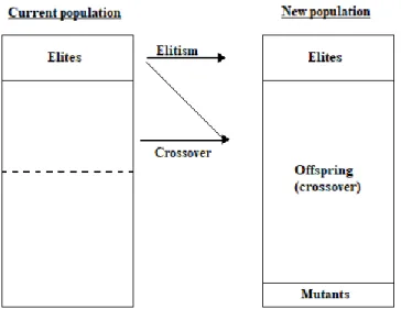
Apart from the mutation operator, we apply standard genetic operators. The population that will make up the subsequent generation will be composed of a group of elites (individuals that have better fitness scores), the offspring that result from the crossover, and a new group of random individuals (mutants) – See Figure 11.

(34)

24

3.4.1. Selection

Selection is used to select the fittest individuals for the next generation based on a fitness function and/or probability (Khouja et al., 1998). In addition, this function is also used to select the parents to be used by the crossover operator.

The literature hasn’t agreed on what is the best parent selection method, depending on the problem, tournament selection and roulette wheel are chosen over the random choice. Regarding lot sizing problems, different authors use different methods. Kimms (1999) creates a pool with the solutions that have better fitness (elites) and then chooses the parents randomly out of the elite pool. However, roulette wheel selection seems to be the most commonly used (Gaafar, 2006; Sarker & Newton, 2002; Xie & Dong, 2002). We applied a similar approach to Kimms. The chromosomes that have above average scores are placed in a pool. From the pool of best performing chromosomes, we pick the parents randomly.

The elite consist of the individuals of a population that have the best fitness scores. Elitism ensures that the best solutions are not lost during the disruptive operation of crossover or mutation. By preserving the best individuals of each generation we can speed up the performance of the GA (Rudolph, 2001; Zitzler et al., 2000). The elitism process is simple. We pick a percentage of the individuals with the highest sum of fitness scores.

(35)

25

The individuals are then copied onto the next generation (Altiparmak, Gen, Lin, & Paksoy, 2006; Dellaert, Jeunet, & Jonard, 2000; Khouja et al., 1998).

In terms of execution of the process, the elite function of the algorithm proposed in this dissertation does not copy directly the result into the next generation. It creates an elite group that will be later merged with the crossover and mutation groups. The result will then be the subsequent generation. The pseudo code of the elitism is given in Figure 12.

procedure 3: Elite population

inputs: population w/ scores :population with the scores assigned

%_elites :percentage of the population to be considered elite

output: elite population: the elite population that will be copied into the next generation

step 1. %_elites  Get the percentage of individuals to consider elite

step 2. n_elite  Get the number of solutions to copy to the next generation (%_elite × POP_SIZE)

step 3. scores  Get the score of each individual

step 4. ind_max  Search in scores for n_elite solutions with the highest scores step 5. elites  Copy the ind_max solutions

Figure 12 – Pseudocode: Elite function.

3.4.2. Crossover

Crossover is applied after two parents are selected, some chromosomes are exchanged to generate the offspring (Melanie, 1999). The crossover technique allows the convergence towards a solution, further exploring the subspace (Grefenstette, 1986).

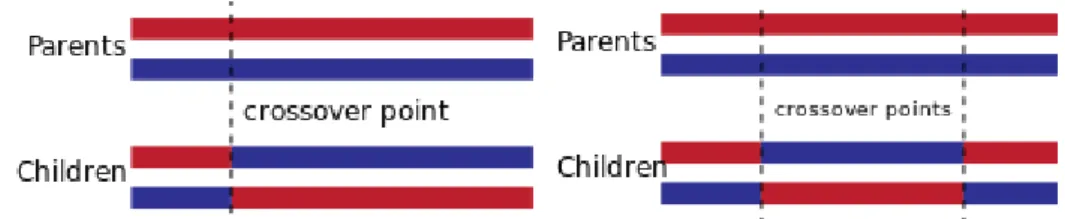
One of the most popular crossover technique is the 2-point crossover. Jong (1975) and David E. Goldberg (1989) favor the 2-point crossover over the 1-point crossover and multi-point crossover. The n-point crossover selects n points on the chromosome and the

information between those points are exchanged between the parents. Figure 135

illustrates the use of 1-point (left) and 2-point (right) crossovers.

5_{Credits of the figure: R0oland (https://commons.wikimedia.org/wiki/File:OnePointCrossover.svg and}

https://commons.wikimedia.org/wiki/File:TwoPointCrossover.svg)

(36)

26

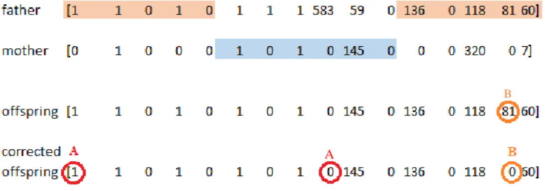
As we said previously, operationally, the algorithm contains a binary component, which represents the decision to send. When we applied the 2-point crossover on the whole chromosome two problems arose. On one half of the chromosome the decision was to send, but no quantities were associated to that decision. The problem is illustrated in Figure 14, marked with the letter A. The other problem was having a quantity to send, but the decision was null (Figure 14, letter B).

To overcome these issues, we need to see both halves as two dependent chromosomes. Thus, the cuts that we make on one, have to be mirrored on the other. Given the size of

both halves, and to avoid disrupting the building block6_{of the chromosome, we used the}

1-point crossover.

We already introduced how the parents are chosen. Furthermore, a random generator will decide which parent gets the first half of the crossover. If the number is lower than 0.5 the “random father” will provide the first half and the “random mother” will fill in the rest. Otherwise, the “mother” gets the first half and the “father” the rest. The parent selection and crossover pseudocode is given by Figure 15.

6_{Building blocks are short, low order and high performing schematas (chromosome’s masks) (Beasley,}

Bull, & Martin, 1993; David E. Goldberg, 1989).

Figure 14 - 2-point crossover issue.

A

(37)

27

procedure 4: Crossover

inputs: population w/ scores :population with the scores assigned

%_crossover :percentage of the new population the be the result of crossover

output: offspring: the offspring resultant of the crossing of two parents from the population.

These will be part of the new generation.

step 1. %_crossover, n_crossover Get the percentage of individuals that will be on the next generation resulting from crossover and respective number.

step 2. parent_pool  Gather the chromosomes that have scores above average. step 3. rnd_father, rnd_mother  Get a pair of random parents from the parent_pool. step 4. If rnd_father = rnd_mother, repeat step 3.

step 5. rnd_factor  Get a random float-point number between 0 and 1.

step 6. If the random factor is < 0.5 the rnd_father chromosome will be on the 1st_{and 3}rd

quarters of the child’s chromosome, and the rnd_mother the remaining. Otherwise, rnd_mother chromosome will be on the 1st and 3rd quarters of the child’s chromosome, and the rnd_father the remaining.

step 7. child  add the offspring to the child array. The array will then be merged with the elite and mutants to form the new population

Figure 15 – Pseudocode: selection of parents and crossover.

3.4.3. Mutants

We use the mutants as an alternative to mutation. Mutation randomly changes (flips) the chromosome (Haupt, 1995). It avoids early convergence to a solution, allowing a broader exploration of the solution space. Instead of changing each chromosome we introduce new random individuals in the population – the mutants or immigrants.

This technique was first introduced by Bean (1994) and used by Toso and Resende (2015) on their biased random-key genetic algorithm. Traditional mutation, when used, disrupts the results of the crossover, that is why it is used with very low probabilities (< 1%). Thus, we are giving a greater role to this operator, and not sacrificing the results of the other genetic operators. These new individuals are created using the same procedure used in generating the initial population. The pseudocode to the mutant procedure is shown by Figure 16.

(38)

28

procedure 5: Mutation

inputs: %_mutants :percentage of the new population to be mutants N_POP :1st_{level population size (nº of stores)}

CHROMO_SIZE :nº of genes in each chromosome

output: mutants: the mutants to be inserted in the new generation

step 1. %_mutants, n_mutants  Get the percentage and number of individuals, respectively, that will be in the next generation as mutants.

step 2. w  random binary array of size N_POP × n_mutants chromosomes. The chromosomes

have a CHROMO_SIZE/2 length

step 3. v  random integer array of size N_POP × n_mutants chromosomes. The chromosomes have a CHROMO_SIZE/2 length

step 4. mutants  concatenate w and v

Figure 16 – Pseudocode: Mutation..

3.4.4. Parameters

To set the parameters we tested values provided by several authors. However, considering we used a different approach with the mutation operator, we will source the parameters of the latter ones from different authors than the population size and generation parameters. The tests were carried out on a machine running Windows 10 64 bits on 2 2.2GHz Intel® Core™ i5-5200U CPUs with access to 6 Gb RAM. The algorithm runs in Python 3.6.0.

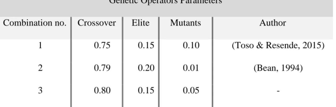
The combinations of the parameters of the genetic operators used are shown in Table 2. Both Toso & Resend and Bean used the mutants successfully in their work so we decided to test the values they have used. However, a third combination is introduced that maintains Toso and Resende’s elite parameter, while giving more weight to the crossover.

Genetic Operators Parameters

Combination no. Crossover Elite Mutants Author

1 0.75 0.15 0.10 (Toso & Resende, 2015)

2 0.79 0.20 0.01 (Bean, 1994)

3 0.80 0.15 0.05 -

Table 3 - Combinations of the genetic operators’ parameters.

In addition to the genetic operators’ parameters, three different population sizes and three generations numbers were tested. The optimal population size is a hard problem

(39)

29

(Eiben, Hinterding, & Michalewicz, 1999), as many factors need to be taken into account, such as: problem difficulty, number and diversity of individuals, and search space among others (Diaz-Gomez & Hougen, 2007). The population size varies between 30 (Xie & Dong, 2002) up to 200 (Khouja et al., 1998). But as we will see, the higher the number of individuals, the slower is the algorithm processing each generation. Table 4 shows the three values of population sizes tested.

Population Size Parameter

Combination no. Population Size Author

1 30 (Xie & Dong, 2002)

2 40 -

3 60 -

Table 4 - Population parameter values.

The number of generations is also an issue that is highly dependent on the problem. Deb and Agrawal (1998) in their work on the interactions among GA parameters, show that large populations require a low number of generations to return good solutions, and vice versa.

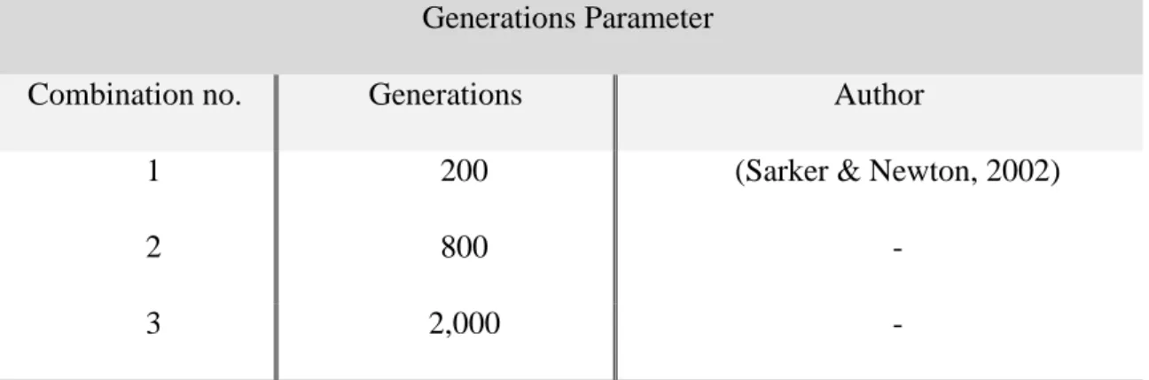
Generations Parameter

Combination no. Generations Author

1 200 (Sarker & Newton, 2002)

2 800 -

3 2,000 -

Table 5 - Generations Parameter.

This setup results in 27 different combinations of parameters. The tests will be done under the same initial setup and run over 25 weeks. The four combinations that yield the lowest costs will run over the 52 weeks and be compared with the method currently being applied by the company. Appendix 3 summarizes the 27 possible combinations.

(40)

30

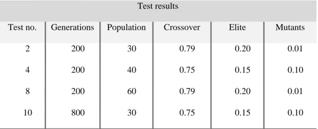
The tests that achieved the lowest costs were tests 2, 4, 8 and 10 (see Table 6). The results show that the algorithm is able to converge rapidly (3 out of the 4 best tests run only 200 generations). Moreover, the best genetic operator combination is split between

Bean and Toso and Resende. Appendix 47 summarizes the results in a table and in

Appendix 5 the results can be visualized.

Test results

Test no. Generations Population Crossover Elite Mutants

2 200 30 0.79 0.20 0.01

4 200 40 0.75 0.15 0.10

8 200 60 0.79 0.20 0.01

10 800 30 0.75 0.15 0.10

Table 6 - Top four test results.

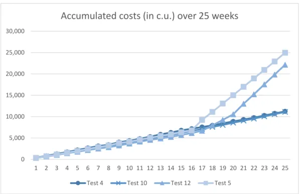
Every test starts with about the same costs. However, by week 13, most of the tests start to increase their costs. These surges are caused by excess of stock in the stores, and later, in the warehouse. The best performing tests seem to send slightly more products over the first weeks (slightly higher costs). Hence, it avoids having large amounts of stock in the warehouse to when large on order quantities arrive.

Figure 17 compares tests 4 and 10 (top performing tests) against tests 5 and 12 (underperforming tests). The surge of the latter ones is not in week 13, as mentioned above, but in week 17 and 18, respectively.

7_{The data of some tests is missing because the increasing costs didn’t justify extending the time}

(41)

31

To select the parameters, we carried out 27 different tests. The algorithm run on 25 different instances of time, i.e. for 25 weeks. In Chapter 4, the best 4 combinations of parameters were then tested during the 52-weeks period and compared with the results of the system that is currently used. We will, henceforth, refer to the tests as combinations.

3.5. Repair function

A repair function is used on the top five solutions, after all the generations are processed, i.e., at the end of each week. The function aims at amending misalignments with the problem restrictions. Although the fitness function also evaluates the admissibility of the solutions, we observed that as the problem progresses in the time, some limitations are, inevitably, not being met (i.e., capacity constraints). Thus, to provide the best solution possible a repair mechanism was introduced. Conditions are addressed in order of importance and once verified, and corrected if needed, they cannot be changed. That is, conditions, verifications and corrections cannot override the previous conditions, and cannot be overridden by the subsequent conditions.

We set as first priority the warehouse capacity. If the capacity is exceeded (recall that for this condition, the predicted on order quantity is accounted for), a coefficient greater

Figure 17- Comparison of two good performing tests with two underperforming tests. 0 5,000 10,000 15,000 20,000 25,000 30,000 1 2 3 4 5 6 7 8 9 10 11 12 13 14 15 16 17 18 19 20 21 22 23 24 25