Numerical modelling of a seal using a ferrofluid to block the passage of lubricating OIL / Modelagem numérica de um selo utilizando um ferrofluido para bloquear a passagem de óleo lubrificante

(1)

Braz. J. of Develop.,Curitiba, v. 6, n. 9, p. 69465-69491, sep. 2020. ISSN 2525-8761

Numerical modelling of a seal using a ferrofluid to block the passage of

lubricating OIL

Modelagem numérica de um selo utilizando um ferrofluido para bloquear a

passagem de óleo lubrificante

DOI:10.34117/bjdv6n9-408

Recebimento dos originais: 14/08/2020 Aceitação para publicação: 17/09/2020

Paulo Cristiano Moro

Institutos Lactec, Curitiba, PR, Brazil

Luiz Alkimin de Lacerda

Rodrigo Paludo

Claiton da Silva Mattos

Renato Penteado

Institutos Lactec, Curitiba, PR, Brazil e-mail: [email protected]

Ernani A. Krüger

Luiz A. J. Procopiak

Companhia Paranaense de Energia, PR, COPEL, Brazil

ABSTRACT

Plain bearings are devices used in large-sized equipment, such as power-generating units. To reduce friction and improve the sustainability of the structure, large quantities of lubricating oil are used in those plain bearings. The heat combined with the turbulent flow causes this lubricating oil to be fragmented and sucked into the generator, thereby damaging its parts. This article reports a study focused on providing a numerical and experimental analysis of a seal prototype using a ferrofluid as the seal agent. To validate the usage of a ferrofluid as a mechanical seal, a prototype was developed and built.

Keywords: Ferrofluid. Magnetic bearing. Finite element method. Lubricating oil steam.

Experimental validation.

RESUMO

Mancais de deslizamento são dispositivos utilizados em equipamentos de grande porte, tais como unidades geradoras de energia. Para reduzir o atrito e melhorar a sustentabilidade da estrutura, grandes quantidades de óleo lubrificante são usadas nesses mancais de deslizamento. O calor

(2)

Braz. J. of Develop.,Curitiba, v. 6, n. 9, p. 69465-69491, sep. 2020. ISSN 2525-8761 combinado com o fluxo turbulento faz com que este óleo lubrificante seja fragmentado e sugado para dentro do gerador, danificando assim suas partes. Este artigo relata um estudo focado em fornecer uma análise numérica e experimental de um protótipo de vedação usando um ferrofluido como agente de vedação. Para validar o uso de um ferrofluido como um selo mecânico, foi desenvolvido e construído um protótipo.

Palavras-chave: Ferrofluido. Mancal magnético. Método dos elementos finitos. Vapor de óleo

lubrificante. Validação experimental.

1 INTRODUCTION

The majority of rotating equipment uses bearings as support. To reduce the friction between the rotating and the static parts in the bearings, high quantities of lubricating oil are used. Due to the exposure to heat and turbulent flow, the lubricating oil can be fragmented and expelled from inside the bearing.

Some problems may occur due to vaporization of the bearing lubricating oil. Condensation of the oil may occur in the stator bars and rotor, which might jeopardize the generator electrical insulation. Vaporization of lubricating oil also may contaminate the environment, leading to labour accidents.

In the past, vaporization of the lubricating oil was a significant problem in the automobile industry. At present, there are successful solutions to this problem, as we can observe by considering the different types of seals on the market. In theory, those same solutions could be applied to large-sized machines, such as the ones used in the electricity generation field. The biggest problem, in this case, is that the rotating rings of the bearings are larger than the ones applied in the automotive industry, which leads to accentuated peripheral velocities.

The problem described in the last paragraph has neither definitive nor efficient known successful solutions, although some solutions reduce the leaking of lubricating oil steam or prevent part of the oil from settling in external surfaces [1].

Therefore, a seal system that offers an efficient seal in the presence of high circumferential velocities combined with high temperatures would be the ideal solution for large-sized equipment. [2].

A ferrofluid, described by [2] and [3], it is a non-Newtonian fluid for which in the presence of a uniform or variable magnetic field, some of its characteristics are changed. In the application described, the most important characteristics that can be changed by the presence of the magnetic field are the stiffness and the viscosity [4].

To verify and qualify the ferrofluid seal, a prototype was developed, built and tested in the lab.

(3)

Braz. J. of Develop.,Curitiba, v. 6, n. 9, p. 69465-69491, sep. 2020. ISSN 2525-8761 To use the ferrofluid as a seal, the presence of a magnetic field in the area of interest is necessary. In the first prototype, a permanent magnet was used to generate the magnetic field, which generated some assembly and maintenance problems that could lead to the impossibility of recreating the equipment on a larger scale.

Therefore, to improve the control of the generation of the magnetic field and solve the problems due to the permanent magnet, an electromagnet was projected and built to generate the magnetic field. The electromagnet prototype was created to block a certain quantity of ferrofluid in the bearing air gap. This air gap consists of a small space between the static and moving parts of the plain bearing to be sealed by the ferrofluid (Figure 1).

Figure 1. Ferrofluid application.

.

The project of the electromagnet and the magnetic circuit was developed using first Maxwell’s equations and later numerical simulations to verify the distribution of the magnetic field through the bearing, making it possible to improve the project.

After the theoretical analysis and the results from the simulations, a final prototype was built and tested to confirm the validity of the model. Figure 2 shows an image of the prototype in lab.

(4)

Braz. J. of Develop.,Curitiba, v. 6, n. 9, p. 69465-69491, sep. 2020. ISSN 2525-8761 Many tests were performed to prove the applicability of the ferrofluid as a mechanical seal. The results, applicability of the technology, limitations and usability will be discussed in this paper.

2 PERMANENT MAGNET SEAL PROJECT

The research was developed to create and build a seal prototype that uses a ferrofluid as a barrier to prevent vaporization of the lubricating oil inside the plain bearings.

To keep the ferrofluid inside the interested area and to determine its viscosity and stiffness, it is necessary to apply a magnetic field to the ferrofluid.

To project the magnet, a theoretical approach using Maxwell’s equations was employed, as shown in [5]. Therefore, an analogy with an electric circuit was used for the theoretical project of the magnetic field distribution.

In the next sections, the development steps will be presented, in addition to the construction and tests of the model that validate the concept and the technology.

3 PERMANENT MAGNET PROJECT

The first project step was the creation of a basic shape based on already successful studies, as in [6].

For this project, a permanent magnet made out of neodymium, iron and boron (NdFeB) was used due to its high magnetic field compared to other materials. The theoretical magnetic circuit of this project is presented in Figure 3.

Figure 3. Theoretical magnetic circuit.

An analogy to an electrical circuit was used to calculate the magnetic circuit, where the reluctance works as a resistance, as can be observed in equation (1).

(5)

( )

1 .S L  = 

Where  stands for the reluctance,  represents the magnetic permeability, L is the path length of the magnetic field, and S is the area through which the magnetic field passes.

The term for the analogy between an electric circuit and the magnetic circuit is the magnetic flux. The following equation presents the relation between the magnetic flux and the density of the electric field lines in a certain area (2).

( )

2 .S

B

= 

where  represents the magnetic flux.

The analogous term for the tension in volts within a magnetic circuit is the magnetomotive force measured in amperes per coil. Using this analogy, it is possible to obtain the Ohm’s law of the magnetic circuit (3):

( )

3 .  = m V where m

V is the magnetomotive force.

Those equations were used to create the geometry for the construction of the prototype for the tests. Figure 4 presents an outline of the interior of the prototype.

Figure 4. Prototype geometry.

In addition to the mathematical analysis using equations (1), (2) and (3), numerical simulations of the magnetic model where performed. Those simulations were performed using the ANSYS software package with the magnetostatic unit [7], as done in [9]. In Figure 5, the magnetic field density in the ferrofluid is shown.

Shaft Magnet

(6)

Figure 5. Density of the magnetic field in the ferrofluid.

In this simulation, the same geometry as in Figure 4 was used, at both ends of the prototype, in order to create a proper test surface.

A polarity test in the magnets was done to verify the best assembly sequence. Two different assemblies were tested, one with the magnetic poles aligned and the other with them in the opposite direction, as shown in Figure 6.

Figure 6. Magnets assembly.

The best configuration, which resulted in the least loss of the magnetic field, was the assembly with opposite pole directions, represented by the second configuration in Figure 6.

4 TESTS AND RESULTS

To verify the efficiency of the ferrofluid as a seal and to analyse the consequences of its usage, the following tests were performed using the permanent magnet model.

The following measurements were made: • Model parts temperature (°C)

• Intensity of the motor supply current (A) • Motor rotation (rpm).

1°

2°

(7)

Braz. J. of Develop.,Curitiba, v. 6, n. 9, p. 69465-69491, sep. 2020. ISSN 2525-8761 The following instruments were used in those measurements:

• A thermal camera • A clamp meter • An AC drive.

The tests were performed in two stages, the first one without ferrofluid and the second one with magnetized ferrofluid. This strategy was used in order to recognize the initial conditions of the model by recognizing the loads generated by the plain bearing friction.

For the tests without ferrofluid, the collected data are reported in Table I.

Table I. Results for the model without ferrofluid.

Variable Results Temperature (Thermal camera) 19,2 ⁰C Current (Motor) 1,6 A Rotation (Motor) 286,7 rpm

In Table II, the results for the model with ferrofluid in the air gap are presented.

Table II. Results for the model with ferrofluid.

Variable Results Temperature (Thermal camera) 20,2 ⁰C Current (Motor) 1,53 A Rotation (Motor) 286,7 rpm

This model had a problem due to the difficulty of assembling and maintaining the system when using the permanent magnet. Once the ferrofluid is locked into the plain bearing, it is difficult to take it off because a magnetic field is needed to do so.

For this reason, no other tests were performed using this model. Project of a seal using an electromagnet

To overcome the difficulties and limitations of the construction of the model with a permanent magnet, a project using electromagnets as the source of the magnetic field was developed.

Electromagnet project

Following the same method as the permanent magnet project, the first step of the electromagnet project was to develop its theoretical model.

(8)

Braz. J. of Develop.,Curitiba, v. 6, n. 9, p. 69465-69491, sep. 2020. ISSN 2525-8761 To use the existing laboratory structure, the first assumption of the electromagnet project is that it should substitute for the permanent magnet, and the others parts of the model should be kept.

With that in mind, the model with the electromagnet should have the same dimensions and characteristics as the model presented in Figure 4. In the electromagnet project, the same concept of an analogy between magnet and electric circuits was used, in addition to the equations shown in [8]. For the electromagnet, we have

( )

4 . 2 . . 0 g I N B=

where B is the magnetic flux density,

0

 is the magnetic permeability in vacuum, N is the number of coils in the electromagnet, I is the current applied to the electromagnet, and g is the distance between the poles.

With that equation, an electromagnet equivalent to the permanent magnet was built with the following characteristics: a ring shape with an internal diameter of 75 millimetres, a width of 6 millimetres and 310 coils made of 0,51-millimetre wire (24WG). To create a magnetic field like the one created in the permanent magnet, a current of 1,3 A was applied.

Using this configuration, numerical simulations were also performed in order to confirm the characteristics of the electromagnet and identify the distribution of the magnetic field in the model.

Figure 7 shows the vector distribution of the magnetic field.

Figure 7. Distribution of the magnetic field in the electromagnet model.

It is possible to observe the assembly of the electromagnet model in Figure 2.

5 TESTS AND RESULTS

(9)

Braz. J. of Develop.,Curitiba, v. 6, n. 9, p. 69465-69491, sep. 2020. ISSN 2525-8761 following variables were measured:

• Magnetic field (gaussmeter) (Gauss)

• Pressure inside the test chamber (pressure gauge) (Pa) • Gas leakage (gas meter).

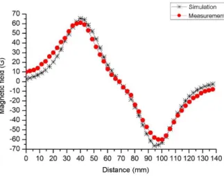
To validate the simulations and the theorical results, measurements of the magnetic field were performed at some locations of the model. Different conditions of electric current were used to perform the cited measurements.

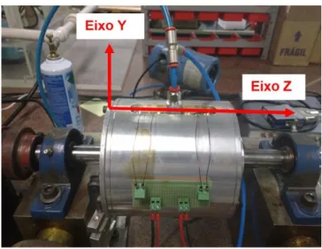
The magnetic field measurement was realized in two different directions due to the fact that it is a vector. This is the reason why those measurements were made in both the axial direction (z direction) and radial direction (y direction). Those directions are shown in Figure 8.

Figure 8. References for the magnetic field measurement.

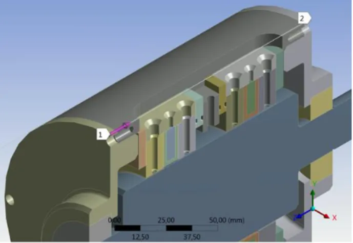
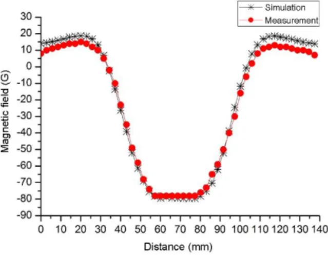
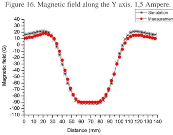
The measurements of the magnetic field were performed at 1,0 A, 1,3 A, 2,0 A and 2,5 A. The results are presented in Figure 10, Figure 11, Figure 12, Figure 13, Figure 14, Figure 15, Figure 16, Figure 17, Figure 18 and Figure 19. The results are presented in the following figures as a function of the distance to the left end of the model (as in Figure 8). The measurement spots are defined according to the simulation results in the same area of the model. To compare the results, the magnetic field in both the X and Y axis directions is presented, as shown in Figure 9.

(10)

Figure 9. Line used to present the results of the finite element method.

Figure 10. Magnetic field along the Y axis. 1,0 Ampere.

(11)

(12)

Figure 15. Magnetic field along the Z axis. 2,0 Ampere.

(13)

From the above figures, it is possible to observe that regarding the Y axis, the difference between the simulated magnetic field and the real measurements is greater than for the Z axis.

The difference in the Y-axis magnetic field can be explained because there is a geometric difference from the model in the area under the influence of a strong magnetic field. This difference occurs mainly due to the refining mesh process and to the approximations made in the mathematical process. Nevertheless, the maximum difference between the simulated and calculate magnetic field is approximately 2%.

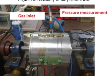
Pressure tests were also performed in between the layers of the ferrofluid in order to verify how much pressure the ferrofluid can maintain inside the model. A gas meter was used to detect leakage in the system, only through the ferrofluid. In order for the gas to be detectable by the installed gas meter, halogen gas was used.

(14)

Braz. J. of Develop.,Curitiba, v. 6, n. 9, p. 69465-69491, sep. 2020. ISSN 2525-8761 inside the test chamber. Tests varying the electric current in the electromagnet and the shaft rotation were performed. The test conditions were the following:

• Electromagnet current: 1,0 A; 1,3 A; 1,5 A; 2,0 A and 2,5 A.

• Shaft rotation: 0 rpm, 300 rpm, 600 rpm, 900 rpm, 1200 rpm, 1500 rpm and 1800 rpm. For each rotation, the measured leakage and pressure in the ferrofluid were recorded. The pressure measured was the gauge pressure, which is the difference between the measured and ambient pressures. The test assembly is shown in Figure 20.

Figure 16. Assembly of the pressure test.

To increase the experimental range, 2 models of ferrofluid were used to realize the pressure and leakage tests: a synthetic-based ferrofluid and a mineral-based one. The characteristics of viscosity and magnetic saturation are reported in Table III.

Table III. Characteristics of the tested ferrofluid.

Model Magnetic Saturation Viscosity (cP) APG S10N 440 300 EFH3 650 12

APG S10N and EFH3 Ferrofluid

The tests were performed at the same current found in the simulations. The results of how much pressure each current can cause the ferrofluid to support are presented next.

(15)

1,0-ampere current

The results of the pressure versus time for rotational speeds of 0 rpm and 300 rpm are shown in Figure 21.

Figure 17. Pressure versus time for 0 and 300 rpm.

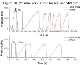
The results of the pressure per time for rotational speeds of 600 rpm and 900 rpm are shown in Figure 22.

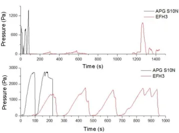
The results of pressure versus time for rotational speeds of 1200 rpm and 1500 rpm are shown in Figure 23.

(16)

Figure 19. Pressure versus time for 1200 and 1500 rpm.

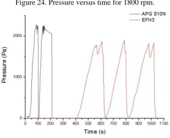
Finally, the results for the pressure versus time for a rotational speed of 1800 rpm are presented in Figure 24.

Figure 20. Pressure versus time for 1800 rpm.

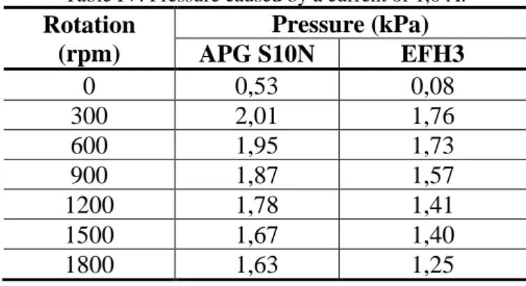
Table IV presents the approximate values of the pressure under a current of 1,0 Ampere.

Table IV. Pressure caused by a current of 1,0 A. Rotation (rpm) Pressure (kPa) APG S10N EFH3 0 0,53 0,08 300 2,01 1,76 600 1,95 1,73 900 1,87 1,57 1200 1,78 1,41 1500 1,67 1,40 1800 1,63 1,25

(17)

(18)

Finally, the results for the pressure versus time for a rotational speed of 1800 rpm are displayed in Figure 28.

Table V presents the approximate values of the pressure caused by a current of 1,3 Ampere.

Table V. Pressure caused by a current of 1,3 A. Rotation (rpm) Pressure (kPa) APG S10N EFH3 0 1,38 0,98 300 2,76 1,76 600 2,70 1,71 900 2,61 1,78 1200 2,50 1,72 1500 2,37 1,81 1800 2,27 1,89

(19)

The results of pressure versus time for rotational velocities of 1200 rpm and 1500 rpm are shown in Figure 31.

(20)

Finally, the results for the pressure versus time for the rotational speed of 1800 rpm are displayed in Figure 32.

Table VI presents the approximate values of the pressure caused by a current of 1,5 Ampere.

Table VI. Pressure caused by a current of 1,5 A.

Rotation (rpm) Pressure (kPa) APG S10N EFH3 0 2,41 0,32 300 3,52 1,58 600 3,38 2,16 900 3,22 2,33 1200 3,08 2,39 1500 2,92 2,47 1800 2,76 2,50

(21)

(22)

Figure 32. Pressure for 1800 rpm.

Table VII presents the approximate values of the pressure caused by a current of 2,0 ampere.

Table VII. Pressure caused by a current of 2,0 A. Rotation (rpm) Pressure (kPa) APG S10N EFH3 0 4,31 0,93 300 4,71 3,37 600 4,65 4,24 900 4,17 4,40 1200 4,06 4,33 1500 3,81 3,88 1800 4,02 3,49

(23)

The results of the pressure versus time for rotational speeds of 0 rpm and 300 rpm are shown in Figure 37.

(24)

Table VIII presents the approximate values of the pressure caused by a current of 2,5 ampere.

Table VIII. Pressure caused by a current of 2,5 A. Rotation (rpm) Pressure (kPa) APG S10N EFH3 0 5,43 0,25 300 6,01 5,81 600 5,82 5,82 900 5,45 5,92 1200 5,23 5,35 1500 5,08 5,15 1800 4,59 4,67

(25)

Braz. J. of Develop.,Curitiba, v. 6, n. 9, p. 69465-69491, sep. 2020. ISSN 2525-8761 The values of the pressures of the APG S10N ferrofluid caused by the applied current can be observed in Figure 41.

Figure 37. Comparison of the response of AP S10N to different currents.

The same data, but for the EFH3E ferrofluid, are displayed in Figure 42.

Figure 38. Comparison of the response of EFH3 to different currents.

6 CONCLUSIONS

As the results show, the usage of a ferrofluid as a mechanical gas seal is possible, although this system only works for a certain range of pressure.

It is also possible to observe that this seal works for rotary systems, such as large-sized plain bearings. Ferrofluid is also a solution for sealing bearings with elevated peripheral velocities, with results similar to or even better than products already on the market.

The assembly of the model and the magnetic field tests and measurements validated the mathematical model. The results were compared with the ones obtained through the finite element method (FEM), demonstrating the applicability and advantages of this method as a solution to

(26)

Braz. J. of Develop.,Curitiba, v. 6, n. 9, p. 69465-69491, sep. 2020. ISSN 2525-8761 static magnetic problems.

ACKNOWLEDGEMENTS

The team acknowledges the support received from everyone involved in the activities and the contributors from Lactec and from the Companhia Paranaense de Energia Elétrica (COPEL) for their attention and dedication to this work.

We acknowledge Professor Doctor Luiz Alkmin de Lacerda for his guidance and support during the research activities. The authors also acknowledge the Brazilian Ministry of Science and Technology (MCT) and the Brazilian National Council for Technological and Scientific Development (CNPq), law 8010.

(27)

REFERENCES

Oliveira, E. F.; Botrel, T. A.; Frizzone, J. A.; Paz, V. P. S. análise hidráulica de hidro-ejetores.

Scientia Agricola, vol. 53, pp. 241–248, 1996.

Scherer, C.; Neto, A. M. F. Ferrofluids — Properties and applications. Brazillian Journal of

Physics, vol. 35, pp. 718–727, 2005.

Raj, K.; Moskowitz, B.; Casciari, R. Advances in ferrofluid technology. Journal of Magnetismand

Magnetic Materials, vol. 149, pp. 174–180, 1995.

Gertzos, K. P.; Nikolakopoulos, P. G.; Papadopoulos, C. A. CFD analysis of journal bearing hydrodynamic lubrication by Bingham lubricant. Tribology International, vol. 41, pp. 1190–1204, 2008.

Hayt, W. H.; Buck, J. A. Eletromagnetismo. 6a Edição ed. Rio de Janeiro, 2001, pp. 132 – 157.

Liu, T.; Cheng, Y.; Yang, Z. Design optimization of seal structure for sealing liquid by magnetic fluids. Journal of Magnetism and Magnetic Materials, vol. 289, pp. 411–414, 2005.

MOAVENI, S. Finite Element Analysis - Theory and Application with ANSYS. Second ed. New Jersey: Prentice Hall, 1999.

Malagoni, J. A.; Steffen Jr, V.; Cavalini Jr, A. A. “Análise da Densidade de Fluxo em um Mancal Magnético via Método dos Elementos Finitos”. UFPR, p. 5, 2016. Pontal do Paraná.

Moro, P. C. “Modelagem numérica de um selo utilizando um ferrofluido como barreira à passagem do óleo lubrificante”. LACTEC, p. 143, 2017. Curitiba.