Early development and metabolic physiology of the temperate lesser spotted shark (Scyliorhinus canicula) under high CO2 levels

2019

UNIVERSIDADE DE LISBOA FACULDADE DE CIÊNCIAS DEPARTAMENTO DE BIOLOGIA ANIMAL

Early development and metabolic physiology of the temperate

lesser spotted shark (Scyliorhinus canicula) under high CO

levels”

Ricardo Sampaio Lopes

Mestrado em Ecologia Marinha

Dissertação orientada por:

Doutor Rui Afonso Bairrão da Rosa

III

Agradecimentos

É verdade sim que a vida proporciona obstáculos e desafios, pois sem estes não teria piada. Cabe-nos a nós fazer frente e tentar ultrapassar com sucesso estes “problemas”. Mas, por vezes, é preciso um empurrão para conseguir dar aquele salto ínfimo necessário para conseguir a superação e este é um caso onde isso se aplica. Espero conseguir tocar todas as pessoas que estiveram “lá” para mim e transmitir o meu obrigado de forma sentida.

Preciso de agradecer ao meu orientador, Rui Rosa, pela disponibilidade e hospitalidade que teve para receber um jovem com um desejo peculiar e também agradecer pelo o que faz e continua a fazer pelo meu futuro como apaixonado por tubarões. À minha “shark” team, Catariana, Marta, Maria Rita que ajudaram sempre e estiveram sempre dispostas a ajudar em qualquer situação, desde a rotinas do dia-a-dia, a conselhos super orientados e esclarecedores. Também, particularizando, ao meu amigo Zé, que não tinha obrigação nenhuma de me ajudar, mas apaixonou-se pela minha pessoa e não resistiu em dar-me uma ajuda preciosa tanto no desenho experimental como análise posterior dos dados. Dentro da sua vida ocupada arranjou espaço para auxiliar um miúdo ingénuo com vontade de conquistar o mundo dos tubarões. Em geral, à equipa toda da Guia - belos almoços na varanda, sempre com boa disposição e palavras encorajadoras.

Numa vertente mais pessoal e familiar, quero agradecer profundamente à minha mãe e ao meu pai. Devo a minha vida a estas duas pessoas porque sem eles eu não estaria a fazer o que estou, e não era o que sou. Criaram-me, educaram-me e sempre deram o suficiente e mais que o suficiente para eu continuar a perseguir os meus sonhos. Devo-lhes esta dissertação e tudo o que fiz até agora. Agradecer também à pessoa mais importante da minha vida, ao meu irmão. Crescemos lado a lado e a cada dia que passa vejo que te estás a tornar um homem, és o meu maior orgulho e um obrigado por teres assistido de perto a todos os meus feitos. Quero referir também as minhas segundas mães, avó Lisete e avó Gabi. Obrigado pelos almoços maravilhosos e aquelas sopas incríveis, as minhas 2 meninas que quando estou a jogar e olho para a bancada lá estão elas, sem perceber nada de hóquei em patins, a sorrir e a bater palmas para o seu neto. Obrigado por estes anos que me acompanharam e é um orgulho enorme vosso neto. Em geral, à minha família toda.

Sem esquecer, 2 pessoas que tenho de referir. Obrigado por me acompanhares há 4 anos, por me teres aturado e estares constantemente a sorrir quando estás comigo. És uma das mulheres que mais respeito na vida e é um orgulho enorme estar ao teu lado como companheiro de vida. Há 4 anos que continuo todo babado a olhar para ti e para essa tua pessoa deslumbrante. Bem dita a hora que te vi a descer a escadaria do C3 com aquelas calças às riscas, o top (I’am na icon) com um casaco de ganga. Esse dia ficou marcado em mim e ficará na minha memória para o resto da minha vida. Obrigado cuqui. Um agradecimento também ao cabeçudo, pelas conversas e pelas tardes no terraço passadas a ver quem tinha mais abdominais, e pela ajuda preciosa que deste nesta última reta. Amizade que já tem muitos anos e que continua por esta vida fora, és grande e cá estarei para tomar conta de ti.

IV Por último, uma pessoa muito especial, a pessoa que me fez apaixonar pela biologia, um professor, que acredito ser um dos poucos profissionais do ensino, que reflete uma paixão enorme naquilo que faz e conseguiu contagiar os alunos. A sua boa disposição e sentido de humor contagiante fazia tudo parecer fácil e simples. Já passaram muitos anos da última vez que tive a honra de assistir a uma aula de biologia, mas a pessoa que eu conheci e o professor que foi ficou marcado na minha pessoa. Ao meu professor de biologia do secundário, Professor Rui Carneiro Martins, um muito obrigado por tudo.

V

Abstract

Although sharks thrive in many different kinds of habitats and evolved to fill many ecological niches across a wide range of habitats, these animals are characterized by the limited capability to adapt rapidly to future climate change. Thus, the objective of the present dissertation was to analyze the potential impact of seawater acidification (OA, high CO2 levels ~1000 µatm) on the early development

and physiology of the temperate shark Scyliorhinus canicula. More specifically, we evaluated OA effects on: i) development time and first feed, ii) Fulton condition of the newborns, iii) survival, iv) routine metabolic rate (RMR), v) maximum metabolic rate (MMR), and vi) aerobic scope (AS). The duration of embrygenesis ranged from 118 to 125 days, and after hatching, the mean number of days to start feeding (i.e. first feeding) varied between 4 and 6 days. In both endpoints there were no significant differences among treatments (i.e. normocapnia and hypercapnia; p >0.05). Juvenile survival (after 150 days post-hatching) also did no change significantly under high CO2 levels (p >0.05). Regarding energy

expenditure rates and aerobic window, there were no significant differences in RMR, MMR, and AS among treatments (p-value > 0.005). In the overall, we argue that these findings are associated to the fact that S. canicula is a benthic, cosmopolitan and temperate shark usually exposed to great variations of abiotic factors, like those experienced in the highly-dynamic western Portuguese coast (with seasonal upwelling events). Although the present dissertation only investigated acclimation processes, it is plausible to assume that this shark species will not be greatly affected by future acidification conditions.

Key words

VI

Resumo

Embora os tubarões proliferam em múltiplos habitats e evoluíram de modo a poder ocupar diversos nichos ecológicos, estes peixes têm uma capacidade adaptativa limitada associada às suas estratégias reprodutivas (e.g. maturação sexual tardia, baixa fecundidade) e de vida (e.g. longevidade elevada). Neste contexto, é de extrema importância analisar os possíveis impactos da acidificação (pCO2

~1000 µatm) na ontogenia inicial (desenvolvimento e fisiologia) do tubarão temperado pata roxa (Scyliorhinus canicula). Mais especificamente, nesta dissertação avaliou-se os efeitos da acidificação no: i) tempo de desenvolvimento (i.e. duração da embriogénese) e primeira alimentação, ii) índice de condição Fulton (dos recém-nascidos), iii) sobrevivência, iv) taxa metabólica basal (RMR), v) taxa metabólica máxima, (MMR) e vi) taxa metabólica normal (AS). A duração do desenvolvimento embrionário variou entre 118 a 125 dias. Após a eclosão, a média de número de dias para o começo da alimentação (i.e. primeira refeição) variou entre 4 a 6 dias. Em ambos os resultados não houve uma diferença significativa entre tratamentos (i.e. normocapnia e hipercapnia; p>0.05). A sobrevivência juvenil (150 dias depois de eclodirem) também não variou significativamente com os níveis de CO2

mais elevados (p>0.05). Quanto às taxas metabólicas e performance aeróbica, também não houve diferenças significativas nos RMR, MMR e AS (p-value >0.005). Em suma, estes resultados sugerem que esta espécie bentónica é resiliente a condições de hipercapnia, o que poderá estar relacionado com o facto destes organismos estarem recorrentemente expostos a grandes variações abióticas na costa ocidental portuguesa (e.g. variações térmicas e de pH associados à sazonalidade do sistema de afloramento). Assim sendo, esta espécie de tubarão temperado não parece vir a ser afetada pelas condições de acidificação dos oceanos projetadas para o final deste século.

VII

Table of Contents

I.1 CARBON DIOXIDE, CARBONATE CHEMISTRY AND OCEAN ACIDIFICATION ... 12

I.2 OCEAN ACIDIFICATION EFFECTS IN THE MARINE BIOTA ... 15

I.2.1 Calcification processes ... 15

I.2.2 Behaviour ... 16

I.2.3 Physiology and metabolism ... 17

I.3 EFFECTS OF OCEAN ACIDIFICATION IN SHARKS ... 18

I.4 STUDIED SPECIES: THE LESSER SPOTTED SHARK (SCYLIORHINUS CANICULA) ... 20

I.4.1 Distribution ... Erro! Marcador não definido. I.4.2 Feeding Ecology ... 20

I.4.3 Reproduction ... 20

OBJECTIVES ... 22

II. MATERIALS AND METHODS ... 23

II.1 ANIMAL COLLECTION AND ACCLIMATION ... 23

II.2 DEVELOPMENT, SURVIVAL AND CONDITION ... 25

II.3 METABOLISM AND AEROBIC SCOPE ... 25

III. STATISTICAL ANALYSES ... 29

IV. RESULTS ... 30

IV.1 DEVELOPMENT, FITNESS AND SURVIVAL ... 30

IV.2 METABOLISM ... 35

V. DISCUSSION ... 38

CONCLUSIONS ... 42

REFERENCES ... 43

VIII

Nomenclature

Acronyms

ppm Parts per million

HNO3 Nitric acid

H2SO4 Sulfuric acid

NH3 Ammonia

IPCC Intergovernmental Panel on Climate Change’s

CaCO3 Calcium carbonate

H+ _Hydrogen

HCO3- Bicarbonate

CO32- Carbonate

GT GigaTon

pH Power of hydrogen

DIC Dissolved Inorganic Carbon

ꭥ Saturation state

pCO2 CO2 partial pressure

IUCN International Union for Conservation of Nature

TL Total Length

RMR Routine Metabolic Rate

MMR Maximum Metabolic Rate

AS Aerobic Scope

IX

List of Figures

FIGURE 1-– A)ATMOSPHERIC CO2 CONCENTRATION FROM 1960 TO 2020.THE RED CURVE REPRESENTS THE DIRECT

MEASUREMENTS OF CO2 IN THE ATMOSPHERE.THE BLACK LINE REPRESENTS THE SEASONALLY CORRECT

DATA.; B)ATMOSPHERIC CO2 CONCENTRATION FROM 2014 TO 2019.RED LINE WITH DIAMONDS SYMBOLS

REPRESENTS THE MONTHLY MEAN VALUES, CENTERED ON THE MIDDLE OF EACH MONTH.THE BLACK LINE WITH THE SQUARES REPRESENTS THE EQUIVALENT, AFTER CORRECTION FOR THE AVERAGE SEASON CYCLE.

ADAPTED FROM NOAA,(2018). ... 12

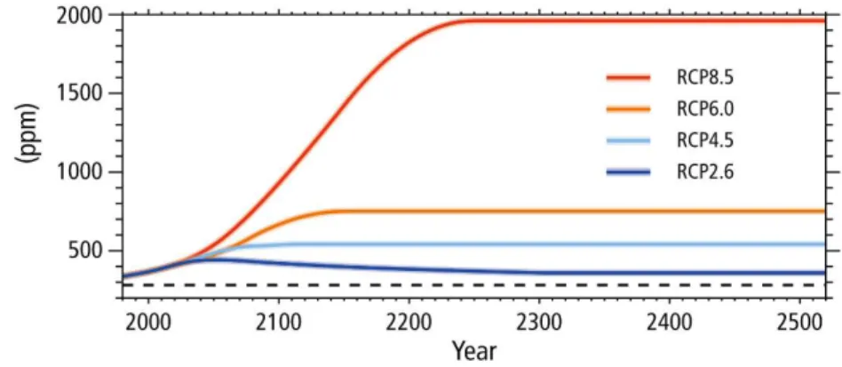
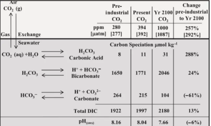
FIGURE 2 – ATMOSPHERIC CO2PROJECTIONS FOR THE FOUR REPRESENTATIVE CONCENTRATIONS PATHWAYS (RCPS).DASHED LINE INDICATES THE PRE-INDUSTRIAL CO2 CONCENTRATION.ADAPT FROM IPCC,(2018). 13 FIGURE 3-THE FATE OF ATMOSPHERIC CO2 AS IT EXCHANGES INTO THE OCEANS AT THE AIR-SEA INTERFACE AND BECOMES PART OF THE AQUEOUS CARBONATE SYSTEM.THE CARBONATE EQUILIBRIUM EQUATIONS ARE SHOWN (LEFT) AND THE CONCENTRATIONS (µMOL KG-1) OF THE DISSOLVED INORGANIC.ADAPTED FROM KOCH ET AL.,(2013). ... 14

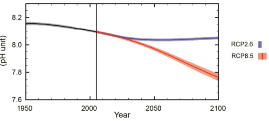
FIGURE 4–GLOBAL OCEAN SURFACE PH FROM 1950 TO 2100 WITH THE 2 POSSIBLE RCP SCENARIOS.THE PURPLE LINE REPRESENTS THE RCP2.6 SCENARIO WHICH ASSUMES A GLOBAL ANNUAL GHG EMISSIONS (MEASURED IN CO2-EQUIVALENTS) PEAK BETWEEN 2010-2020, WITH EMISSIONS DECLINING SUBSTANTIALLY THEREAFTER;AND THE ORANGE LINE REPRESENTS THE RCP8.5 SCENARIO WHICH ASSUMES A CONTINUES GROWTH THROUGHOUT THE 21ST _{CENTURY.ADAPTED FROM EEA,(2018) ... 15}

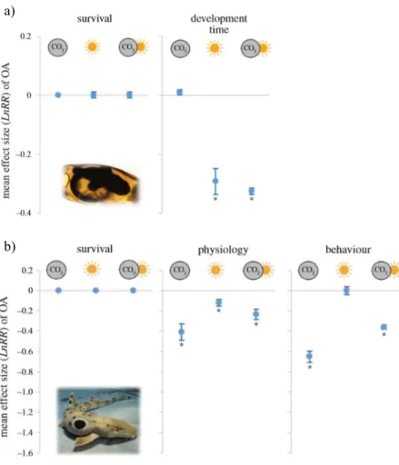
FIGURE 5-DIFFERENCES IN THE MEAN EFFECT OF NEAR-FUTURE CO2 AT CONTROL AND ELEVATED TEMPERATURE CONDITIONS FOR THE DIFFERENT BIOLOGICAL RESPONSE VARIABLES OF, A) EMBRYOS AND, B) JUVENILES. ADAPT FROM ROSA ET AL.,(2017). ... 19

FIGURE 6-GEOGRAPHIC DISTRIBUTION OF THE LESSER SPOTTED SHARK (SCYLIORHINUS CANICULA). ... 20

FIGURE 7- PROTECTIVE EGG CASE OF THE S. CANICULA SHARK. ... 21

FIGURE 8–NEW-BORN S. CANICULA SHARK. ... 21

FIGURE 9 - OCEAN ACIDIFICATION-RELATED EXPERIMENTAL DESIGN FOR THE EGGS AND JUVENILES OF SCYLIORHINUS CANICULA. ... 24

FIGURE 10-GENERAL RESPIROMETRY SETUP FOR S. CANICULA.LEGENDS:A) FLUSH DEPOSIT WITH A WATER PUMP; B) SUMP WITH THERMOSTAT AND WATER PUMP;C) REFRIGERATOR; D)U.V LIGHT; E) SEALED ACRYLIC CHAMBER; ... 26

FIGURE 11--SCHEMATICS OF THE INTERMITTENT FLOW RESPIROMETRY SYSTEM USED FOR THE ASSESSMENT OF OXYGEN CONSUMPTION RATES IN S. CANICULA.LEGENDS:F)“FIRESTING”– FIBRE-OPTIC OXYGEN METER;G) OXYGEN SENSOR;H) WATER PUMPS;I)FLUSH DEPOSIT;BLACK ARROWS REPRESENT THE FLUX. ... 27

FIGURE 12-DEVELOPMENT TIME (DAYS) OF SHARK’S EMBRYOS (SCYLIORHINUS CANICULA) UNDER CONTROL (N=14) AND ACIDIFICATION (N=24) CONDITIONS. ... 30

FIGURE 13-FIRST FEED (IN DAYS) OF S. CANICULA NEW-BORNS EXPOSED TO CONTROL (C-C: CONTROL TO CONTROL; N =13) AND ACIDIFICATION CONDITIONS (C-A: CONTROL DURING EMBRYOGENESIS AND ACIDIFICATION AFTER HATCHING, N =13; A-A: ACIDIFICATION DURING EMBRYOGENESIS AND AFTER HATCHING, N =10). ... 31

X

FIGURE 14-SURVIVAL PROBABILITY THROUGH TIME (DAYS) FOR THE 3 TREATMENTS OF THE JUVENILE SHARKS

(SCYLIORHINUS CANICULA).LEGEND: C-C: CONTROL TO CONTROL; C-A: CONTROL DURING EMBRYOGENESIS AND ACIDIFICATION AFTER HATCHING; A-A: ACIDIFICATION DURING EMBRYOGENESIS. ... 32

FIGURE 15-FULTON CONDITION INDEX COMPARISON BETWEEN TREATMENTS IN 3 LIFE STAGES (HATCH MOMENT, 30 DAYS POST-HATCHING,60 DAYS POST-HATCHING). ... 33 FIGURE 16- ROUTINE METABOLIC RATES (RMR; MG O2KG-1 WW H-1) OF JUVENILE SHARKS (SCYLIORHINUS

CANICULA) UNDER CONTROL (C-C: CONTROL TO CONTROL; N=7) AND ACIDIFICATION CONDITIONS (C-A:

CONTROL DURING EMBRYOGENESIS AND ACIDIFICATION AFTER HATCHING; N=6; A-A: ACIDIFICATION DURING EMBRYOGENESIS AND AFTER HATCHING; N=7) ... 35

FIGURE 17-MAXIMUM METABOLIC RATES (MMR; MG O2KG-1 WW H-1) OF JUVENILE SHARKS (SCYLIORHINUS

CANICULA) UNDER CONTROL (C-C: CONTROL TO CONTROL; N=7) AND ACIDIFICATION CONDITIONS (C-A:

CONTROL DURING EMBRYOGENESIS AND ACIDIFICATION AFTER HATCHING; N=6; A-A: ACIDIFICATION DURING EMBRYOGENESIS AND AFTER HATCHING; N=7). ... 36 FIGURE 18-AEROBIC SCOPE (MG O2KG-1 WW H-1) OF JUVENILE SHARKS (SCYLIORHINUS CANICULA) UNDER CONTROL

(C-C: CONTROL TO CONTROL; N=7) AND ACIDIFICATION CONDITIONS (C-A: CONTROL DURING EMBRYOGENESIS AND ACIDIFICATION AFTER HATCHING; N= 6; A-A: ACIDIFICATION DURING EMBRYOGENESIS AND AFTER HATCHING; N=7). ... 37 FIGURE 19 - TIME-RELATED CHANGES (DAYS) IN FULTON CONDITION INDEX (K) OF JUVENILE SHARKS

(SCYLIORHINUS CANICULA) UNDER CONTROL (C-C: CONTROL TO CONTROL) AND ACIDIFICATION CONDITIONS (C -A: CONTROL DURING EMBRYOGENESIS AND ACIDIFICATION AFTER HATCHING; A-A: ACIDIFICATION DURING EMBRYOGENESIS AND AFTER HATCHING). ... 52

XI

List of Tables

TABLE 1-SEAWATER PHYSIOCHEMICAL PARAMETERS IN THE TWO TREATMENTS: CONTROL AND ACIDIFICATION. ALKALINITY AND PCO2 VALUES REPRESENT MEAN PER TREATMENT ±SD. ... 24

TABLE 2-RESULTS OF THE GENERALIZED LINEAR MIXED MODELS (GLMM) ANALYSIS COMPARING THE CONTROL AND ACIDIFICATION TREATMENTS FOR EMBRYO DEVELOPMENT TIME.VALUES OF P<0.05 ARE SHOWN IN BOLD. ... 30 TABLE 3-RESULTS OF GENERALIZED LINEAR MIXED MODELS (GLMM) ANALYSIS FOR THE FIRST FEED UNDER

CONTROL (C-C: CONTROL TO CONTROL) AND ACIDIFICATION CONDITIONS (C-A: CONTROL DURING EMBRYOGENESIS AND ACIDIFICATION AFTER HATCHING; A-A: ACIDIFICATION DURING EMBRYOGENESIS AND AFTER HATCHING).VALUES OF P<0.05 ARE SHOWN IN BOLD. ... 31

TABLE 4-RESULTS OF GENERALIZED LINEAR MIXED MODELS (GLMM) ANALYSIS FOR THE SURVIVAL OF S.

CANICULA JUVENILES (SCYLIORHINUS CANICULA). ... 32 TABLE 5-GENERALIZED LINEAR MIXED MODELS (GLMM) ANALYSIS RESULTS FOR THE INTERACTION BETWEEN

THE 3 TREATMENTS WITH TIME FOR THE SHARKS FULTON CONDITION.VALUES OF P<0.05 ARE SHOWN IN BOLD. ... 34 TABLE 6-RESULTS OF GENERALIZED LINEAR MIXED MODELS (GLMM) ANALYSIS FOR THE ROUTINE METABOLIC

RATES (RMR MG O2KG-1 WW H-1) OF JUVENILE SHARKS (SCYLIORHINUS CANICULA) EXPOSED TO CONTROL (C

-C: CONTROL TO CONTROL) AND ACIDIFICATION CONDITIONS (C-A: CONTROL DURING EMBRYOGENESIS AND ACIDIFICATION AFTER HATCHING; A-A: ACIDIFICATION DURING EMBRYOGENESIS AND AFTER HATCHING)..

VALUES OF P<0.05 ARE SHOWN IN BOLD. ... 35

TABLE 7-TABLE 7–RESULTS OF GENERALIZED LINEAR MIXED MODELS (GLMM) ANALYSIS FOR THE MAXIMUM METABOLIC RATES (MMR; MG O2KG-1 WW H-1) OF JUVENILE SHARKS (SCYLIORHINUS CANICULA) EXPOSED TO

CONTROL (C-C: CONTROL TO CONTROL) AND ACIDIFICATION CONDITIONS (C-A: CONTROL DURING EMBRYOGENESIS AND ACIDIFICATION AFTER HATCHING; A-A: ACIDIFICATION DURING EMBRYOGENESIS AND AFTER HATCHING)..VALUES OF P<0.05 ARE SHOWN IN BOLD. ... 36 TABLE 8-RESULTS OF GENERALIZED LINEAR MIXED MODELS (GLMM) ANALYSIS FOR THE AEROBIC SCOPE (AS; MG O2KG-1 WW H-1) OF JUVENILE SHARKS (SCYLIORHINUS CANICULA) EXPOSED TO CONTROL (C-C: CONTROL TO

CONTROL) AND ACIDIFICATION CONDITIONS (C-A: CONTROL DURING EMBRYOGENESIS AND ACIDIFICATION AFTER HATCHING; A-A: ACIDIFICATION DURING EMBRYOGENESIS AND AFTER HATCHING)..VALUES OF P<0.05 ARE SHOWN IN BOLD. ... 37 TABLE 9–SUMMARY OF THE AVAILABLE EXPERIMENTALLY BASED STUDIES IN METABOLIC PERFORMANCE ON THE

IMPACTS OF OA IN CARTILAGINOUS AND BONY FISHES.ABBREVIATIONS:C, CONTROL;T, TREATMENT;R-H, RECENTLY HATCHED;NA, NOT APPLICABLE;AS, AEROBIC SCOPE;RMR, ROUTINE METABOLIC RATE;MMR

MAXIMUM METABOLIC RATE. ... 39 TABLE 10–(CONTINUED.) ... 40

12

I.

Introduction

I.1 Carbon dioxide, carbonate chemistry and ocean acidification

The exponential expansion of human activities is threatening marine diversity at a global scale (Dulvy et al. 2014). There are clear evidences that human impacts over the past ten millennia have profoundly and permanently altered biodiversity (Hoffmann et al. 2010). More recently, and over the past 250 years, atmospheric carbon dioxide (CO2) levels increased nearly 130 ppmv (parts per million

volume), from the preindustrial period, 280 ppmv, to 2018, approximately 410 ppmv (NOAA, 2018) (see Fig. 1). Due to, a constant natural resource overexploitation and the use of human fossil combustion (main issues linked to the atmospheric CO2 increase) a dramatic 40% growth on the CO2 levels is

observed.

This rate of CO2 increase is at least an order of magnitude faster than has occurred for millions

of years, and therefore the current CO2 levels are considered to be the highest concentration on the Earth

for at least the past 800,000 years (Doney and Schimel 2007; Lüthi et al. 2008). Climate projections are crucial in order to understand possible future impacts and create adaptations assessments. The Representative Concentration Pathways (RCPs) describe four different 21st century pathways of greenhouse gas (GHG) emissions and atmospheric concentrations, air pollutant emissions and land use. They include a stringent mitigation scenario (RCP2.6), where the global annual GHG emissions peak happens between 2010–2020, with emissions declining substantially thereafter; two intermediate scenarios (RCP4.5 and RCP6.0), where the emissions peak happens in 2040 and 2080, respectively, and

Figure 1 - a) Atmospheric CO2 concentration from 1960 to 2020. The red curve represents the direct measurements of

CO2 in the atmosphere. The black line represents the seasonally correct data.; b) Atmospheric CO2 concentration from 2014 to

2019. Red line with diamonds symbols represents the monthly mean values, centered on the middle of each month. The black line with the squares represents the equivalent, after correction for the average season cycle. Adapted from NOAA, (2018).

13 then decline; and one scenario with very high GHG emissions (RCP8.5), where emissions continue to rise throughout the 21st century(see Fig.2).

Figure 2 – Atmospheric CO2 projections for the four representative concentrations pathways (RCPs). Dashed line

indicates the pre-industrial CO2 concentration. Adapt from IPCC, (2018).

Both in the air and in surface waters the CO2 concentration tend to reach to an equilibrium

(Pörtner, Langenbuch, and Reipschläger 2004b). It is inevitable to discuss the anthropogenic CO2

increase rate and the ocean role without referring the carbonate system. Seawater carbonate chemistry is governed by a series of abiotic chemical reactions and biologically mediated reactions. For the chemical reactions, we have CO2 dissolution and the acid/base chemistry and biologically reactions,

photosynthesis, respiration, and CaCO3 precipitation and dissolution, which depend on the stability of

abiotic parameters such as ocean temperature and alkalinity (Feely, Doney, and Cooley 2009). Is this flux between, air-sea, that maintain the right equilibrium in the carbon chemistry and allows the environment to experience the ideal conditions for all the ecological and biological processes to take place (Munday 2014). Seawater carbonate chemistry is governed by a series of chemical reactions:

CO2(atmos) ↔ CO2(aq) + H2O ↔ H2CO3 ↔ H+ + HCO3- ↔ 2H+ + CO32-

After gas intake in the ocean surface, the CO2 initiate a series of chemical reactions. This

atmospheric compound reacts with a water molecule (H2O) to produce carbonic acid (H2CO3).

Subsequently, H2CO3 dissociate with a release of a hydrogen ion (H+) to form bicarbonate (HCO3-).

Lastly, HCO3- dissociate into carbonate (CO32-) yet with the release of 2 H+ to ocean (Doney et al. 2009).

These seawater chemical reactions are reversible and close to the equilibrium (Millero et al. 2006). Oceans have absorbed approximately half of all anthropogenic CO2 emissions to the atmosphere

due to their large volume and capacity to buffer CO2 seawater, which represents more than 120 GT

(GigaTon) of Carbon in total or 440 GT CO2 within the last 200 year as was mentioned before (see fig.1)

(Sabine et al. 2004). Buffering atmospheric CO2 is one of the many ocean functions. Other examples

14 weather patterns, global climate with the marine photosynthetic organism, heat storing ability, regional climate, and others Earth’s processes.

Ocean acidification (OA) is related to the decrease in pH over an extended period, typically decades, caused primarily by the uptake of CO2 from the atmosphere (Gattuso et al. 2011). It will take

more than ten thousand years for the ocean chemistry returns to a scenario that happened in the pre-industrial period, about 200 years ago (Elderfield et al. 2005).

Figure 3 - The fate of atmospheric CO2 as it exchanges into the oceans at the air-sea interface and becomes part of

the aqueous carbonate system. The carbonate equilibrium equations are shown (left) and the concentrations (µmol kg-1_{) of the}

dissolved inorganic. Adapted from Koch et al., (2013).

Oceans water surface has already acidified by an average of 0.1 pH units from pre-industrial levels. Surface water pH reductions could range from 0.2 units if 1,200 GT C (1 GT = 1015 g) are released over 1000 years to nearly 0.8 units if 5,000 GT C are released over 200 years. Projections based on two different scenarios (RCP 2.6 and RCP 8.5) reveal 2 outcomes. For RCP 2.6 (emissions declining substantially after 2020) is shown an ocean pH stabilization throughout the years. For the second scenario and more drastic, RCP 8.5 (continues growth of CO2 emissions throughout the 21st century)

15 Figure 4 – Global ocean surface pH from 1950 to 2100 with the 2 possible RCP scenarios. The purple line represents the RCP 2.6 scenario which assumes a global annual GHG emissions (measured in CO2-equivalents) peak between

2010-2020, with emissions declining substantially thereafter; And the orange line represents the RCP 8.5 scenario which assumes a continues growth throughout the 21st _{century. Adapted from EEA, (2018)}

There is an considerable interest in understanding how the projected changes in carbonate chemistry will affect marine species, communities, and ecosystems (Kroeker et al. 2013). Due to a reduction in biodiversity caused by the loss of sensitive species that play essential roles in energy flow (i.e. food web function) or other processes (e.g. ecosystem engineers), significant and rapid environmental changes are expected to decrease the stability and productivity of the ocean, therefore, these predicted changes could lead to profound ecological shifts in marine ecosystems (Cardinale et al.

2006; Kroeker et al. 2010). OA has been shown to affect marine organism’s survival, physiology,

behaviour, life history and development. However, physiological responses among taxa have been demonstrated to be extremely variable (Christen et al. 2013). The relative differences in sensitivity to ocean acidification within groups of organisms are likely to lead to changes in community structure, diversity, dynamics and functions, ultimately leading to changes in ecosystem functions (Medina et al. 2007; Pelejero et al. 2010).

I.2 Ocean acidification effects in the marine biota

Susceptibility to calcification is an important issue that cause divergent biological responses to ocean acidification. This issue may be especially sensitive because the carbonate system affects directly the deposition and dissolution rates of the CaCO3 used for structures (Gattuso and Buddemeier 2000).

Calcifying organisms exert a variable degree of control over biomineralisation, which involves a constant ion movement flux in and out of a calcification compartment isolated, passively or actively, from ambient seawater (Dove et al. 2003). Reduced calcification rates are observed following

16 acidification for a variety of calcareous organisms even when aragonite or calcite (saturation state) Ω > 1.0 (Kleypas et al. 2006; Fabry 2008).

A series of chemical reactions is started when CO2 is absorbed by seawater:

ꭥ = ([𝐶𝐴 ][𝐶𝑂 ])/𝐾∗

Where the Ω is the calcium carbonate saturation; 𝐾∗ _{is the stoichiometric solubility product for}

CaCO3and [Ca2+] and [CO32-] are the in-situ calcium and carbonate concentrations, respectively. The

final products of these reactions are an increase in hydrogen ion concentration (H+_{), which lowers pH}

(acid water), and a reduction in the number of carbonate ions (CO32-) available. This decrease in

carbonate ion concentration also leads to a reduction in calcium carbonate saturation state (Ω), which has significant impacts on marine calcifiers, i.e. organisms that construct shells and skeletons from this mineral (Guinotte and Fabry 2008a; Ries et al. 2009a).

Marine calcifiers are among the most sensitive to pH changes, because they highly depend on the mineral form of CaCO3, with the solubility and susceptibility increasing from low-magnesium calcite

to aragonite and high-magnesium calcite (Morse et al. 2006; Ries et al. 2009b). The secretion of CaCO3

skeletal structures is widespread across animal phyla and evolved independently and repeatedly over geologic time since the late Precambrian period (Knoll 2003). However, some species may have the capacity to control pH near calcification sites bellow differing external conditions and thereby may possess better equipped to deal with OA. There will always be “winners”, organism better adapted to new and change abiotic conditions, and the “losers”, where the stress factors are not favourable for their ecological and physiological conditions (Kroeker et al. 2010).

I.2.2 Behaviour

To predict the detrimental impact of OA on animal behavior is essential understand the mechanisms by which sensory and behavioral responses to environmental cues become modified by exposure to CO2-enriched conditions. Sharks are organisms with superior sensorial structures when

compared to teleost fishes, and their specialized structures related to olfactory and electroreceptor systems need to be working effectively to perform the daily basis routines such as prey detection and navigation (Gardiner et al. 2014). According to Rosa et al. (2017), sharks behaviour is affected by warming and water acidification. From hunting behaviour to absolute lateralization, these organisms have showed that their sensorial capabilities and swimming performance are significantly affected under climate change (Dixson et al. 2015; Green and Jutfelt 2014).

The wide range of behavioral responses to OA observed in marine teleosts have been attributed to the relationship acid-base regulation, high CO2 environment and the function of the GABA-A

receptor, the primary inhibitory neurotransmitter receptor in the vertebrate brain (Rosa, Rummer, and Munday 2017). This GABA-A receptor is structure that allow ion movement (CL2 and HCO3) through

17 a membrane resulting in a hyperpolarization or depolarization. Under normal condition ion inflow leads to membrane hyperpolarization and inhibited neural activity. Under acidification scenarios, marine teleosts have a regulator capacity that implies make regulatory adjustments in blood and tissues that affect such transmembrane gradients in some neurons. Regarding this CO2 high scenario, GABA-A

receptors became depolarizing and excitatory, resulting in behavior impairments. This same mechanism situation is applied to sharks. They possess the same receptors (GABA-A) and accumulate HCO3 from

the environment in exchange for Cl2 from the body to buffer eventual pH disturbance (Heuer and Grosell

2014b; Rosa, Rummer, and Munday 2017)

Thus, sensorial biology is affected directly with OA, and shark behaviour that depend on olfactory, audition and other mechanism will also be possibly impacted negatively under OA.

I.2.3 Physiology and metabolism

Metabolism is a crucial component of an organism’s daily energy budget and may account for its highest, yet most variable proportion (Lowe 2001). To sustain an efficient aerobic metabolism, O2

intake and CO2 excretion is essential, where O2 is mandatory for maximal aerobic conversion of food to

energy (Carrier, Musick, and Heithaus 2004). As it is known, many marine organisms show a strong dependency with the surrounding environment, and any abiotic variation will elicit some repercussions in their physiology. For instance, they are more susceptible to an increase in environmental CO2

concentration than terrestrial animals, because of the lower pCO2 of their body fluids (Gordon and

Donald 1996).

Elevated CO2 partial pressures (hypercapnia) will affect the physiology of water breathing

animals by inducing acidosis in the tissues and body fluids of marine organisms. This process called acidosis occurs due to elevated blood pCO2. As the pCO2 in water rises, the pCO2 in animal’s tissues

also rises (Burnet 1997). The main reason for this equilibrium is driven by the osmotic regulation between the organism and the environment. Exist a continuous exchange of ions to the point that both parts achieved an equilibrium (Fabry et al. 2008). PH, bicarbonate, and CO2 levels within the organism

are altered with long-term effects on metabolic functions, growth, and reproduction, all of which could be harmful at population and species levels (Guinotte and Fabry 2008).

Hypercapnia can affect the organism metabolism via acid-base disturbances. Acid-base regulation maybe passive when it is achieved through the increase of bicarbonate ions in intra and extracellular space (Spicer, Raffo, and Widdicombe 2007). Organisms that have high activities of anaerobic metabolic enzymes, consequently, have high capacity for buffering pH (Fabry et al. 2008). Nonetheless, if the equilibrium organism-environment is not achieved in hypercapnia conditions, some studies indicate that some species show suppression in the metabolism as an adaptive strategy to survive (Hand 1991; Pörtner, Langenbuch, and Reipschläger 2004b). One suppression mechanism example is the shutting down of expensive processes, such as protein synthesis (Hand 1991). Yet, passive buffering

18 and shutting down processes are not suffice under chronic long-term hypercapnic scenarios (Pörtner, Langenbuch, and Reipschläger 2004b).

I.3 Effects of ocean acidification in sharks

Although sharks thrive in many different kinds of habitats and evolved to fill many ecological niches across a wide range of habitats, these animals are characterised by the limited capability to adapt rapidly to future climate change, because they display: i) low fecundities, ii) extensive gestation periods (some of highest levels of maternal investments in the animal kingdom), iii) low population growth rates and iv) long-life span, contrary to most marine fish that evolve to a R-selected life-history strategy (Dulvy et al. 2014; Rosa et al. 2016).

All these traits reduce sharks’ capacity to recover once populations are depleted. This is a problem in a way that the human ocean footprint is shown no signs of slowing down. Examples of declining shark populations have been well documented, and approximately 20% of Chondrichthyans species assessed by theInternational Union for Conservation of Nature (IUCN) are considered to be threatened (Chin et al. 2010).

Due to the sharks’ evolutionary history, it was expected that these organisms should be strongly tolerant to high CO levels (Rummer and Munday 2017). In fact, until recently, there was no empirical evidence that sharks were physiologically vulnerable to elevated CO2 (Johnson et al. 2016). Yet,

nowadays there are several studies pointed out that shark physiology and behaviour are indeed affected by OA and global warming (see review in Rosa et al. 2017; Fig. 4).

19 Figure 5 - Mean effect of near-future CO2 at control and elevated temperature conditions for different biological

response variables (namely survival, physiology and behaviour) of: a) embryos and, b) juveniles. Adapt from Rosa et al., (2017).

a)

20

I.4 Studied species: the lesser spotted shark (Scyliorhinus canicula)

Scyliorhius canicula (Linnaeus, 1758), widely known as lesser spotted dogfish, is a small, temperate, bottom-dwelling marine animal (Ellis et al. 2005) This shark species is cosmopolitan with a geographic range from the Northeast and Eastern central Atlantic, the Shetland Islands and Norway in the North, to Western Africa (Morocco, Western Sahara and Mauritania to Senegal, possibly along the Ivory Coast) in the South, including the Mediterranean Sea. It occurs from the shore up to the uppermost slopes, but it is found most commonly in sandy, coralline, algal, gravel or muddy subtracts (Ellis and Shackley 1997).

Figure 6 - Geographic distribution of the lesser spotted shark (Scyliorhinus canicula).

I.4.2 Feeding Ecology

S. canicula is an omnivorous, opportunistic and also a scavenger species , whose diet includes a variety of benthic and pelagic organisms (Olaso et al. 2005), specially crustaceans . Thus, S. canicula plays an essential role as a benthic predator, controlling the benthic fauna belonging to their trophic web. Yet, it is not considered a top predator because given its size they are part of other predators diet (Ellis, Pawson, and Shackley 1996)

I.4.3 Reproduction

Sharks display different reproductive strategies, including: i) an oviparous reproductive process - where female produce eggs that mature and hatch after being expelled from the body, ii) a viviparous process - where embryo development take place inside the parent body, eventually leading to live birth,

21 and iii) ovoviviparous system, where embryos develop inside eggs but remain in the parent body until they hatched.

S. canicula is an oviparous species and lays its eggs in a protective egg case (Fig 7). These egg case contributes to the embryo protection from outside threats and allows the yolk storage inside the case. The egg case is constructed mainly from collagen-containing fibrils with a unique crystalline arrangement (Iconomidou et al. 2007).

Figure 7 - Protective egg case of the S. canicula.

Gestation lasts approximately 5-11 months depending on the surrounding environment, and the sex ratio of recently hatched juveniles is about 1:1. Regarding the birth size, a juvenile can go from 7 to 11 cm total length (Ellis and Shackley 1997) (see Fig.8).

22

Objectives

The objective of the present dissertation was to analyse the possible impacts of ocean acidification (OA; high 𝐶𝑂 levels ~1000 µatm) on the early development and physiology of the temperate benthic shark Scyliorhinus canicula. More specifically, we investigated OA effects on: i) development time (i.e. embryogenesis duration) and first feed, ii) Fulton condition of the new-borns, iii) survival, iv) routine metabolic rate (RMR), v) maximum metabolic rate (MMR), and vi) aerobic scope (AS).

23

II. Materials and methods

II.1 Animal collection and acclimation

Lesser spotted dogfish eggs (S. canicula) were caught between June and August 2017 from adults kept in our facilities (Laboratório Marítimo da Guia - Cascais, Portugal). The adults had been previously caught by local fisherman (using fish traps) in Figueira da Foz (Portugal). Eggs were suspended in a 600L recirculating aquaculture system (by the egg’s long tendrils), with a continues salt water flux from a storing water tank placed outside of the facilities (drip-system), at one of two experimental conditions until hatching: control (~400 μatm, n=28), and acidification (~900 μatm, n=11; Table 1). After hatching, each shark from the control was randomly assigned to one of the two experimental conditions: control (~400 μatm, n=14) and acidification (~900 μatm, n=14) during ~ 100 days (post-hatching). The juveniles that hatched under OA were maintained only under that same condition (Fig. 9). All sharks were photograph after hatching, measured and weighted. They were fed between 2 to 4 time a week with squid mantle and horse mackerel in a 30-minute period (then the tank was cleaned to remove the remain wasted food and metabolic products). The pH values were adjusted automatically through a Profilux controlling system (Kaiserslautern, Germany) connected to individual pH probes. pH values were monitored every two seconds and downregulated by injection of a certified CO2 gas mixture (Air Liquid, Portugal) via solenoid valves, connected to air stones, or upregulated by

aerating the tanks with air. Hysteresis maintained pH levels at ± 0.05 margins. To verify the tank’s pH and, if necessary, adjust the set points of the systems, pH was manually controlled daily with a portable pH probe (SevenGo pro SG8, Mettler Toledo). Seawater carbonate system speciation was calculated weekly from total alkalinity, measured by spectrophotometry (Shimadzu XXXXX) at 595 nm, and pH measurements (Sarazin, Michard, and Prevot 1999). Total dissolved inorganic carbon (CT), pCO2,

bicarbonate concentration and aragonite saturation were calculated using the CO2SYS software (Lewis

and Wallace 1998), with dissociation constants from Mehrbach et al. (1973) as refitted by Dickson and Millero (1987). Water quality and adequate carbonate speciation were obtained using a drip-system, already mentioned before, fitted to the tanks, providing a daily 50% water change with new filtered and UV-sterilized seawater. To achieve a good quality of the other 50% daily water was used a protein skimmer (Schuran, Jülich, Germany), wet-dry filters (BioBalls) and 30 W UV-sterilizers (TMC, Chorleywood, UK). To secure the optimal temperature for the shark’s metabolism was utilised chillers to cool down the water and 2 heaters per tank to warm up. Temperature and salinity were monitored daily with a thermometer and a refractometer, respectively. To simulate the photoperiod that sharks are exposed in their natural environment, 12 hours light: 12 hours dark. The ammonia and nitrites levels were monitored 4 to 5 days a week with an ammonia kit (tropic marine) and kept bellow detectable levels.

24 Figure 9 - Ocean acidification-related experimental design for the eggs and juveniles of Scyliorhinus canicula.

Table 1 - Seawater physiochemical parameters in the two treatments: control and acidification. Alkalinity and pCO2

values represent mean per treatment ± SD.

Control Acidification

Temperature (ºC) 18 ± 0.5 18 ± 0.5

pH 8.0 ± 0.05 7.7 ± 0.05

Photoperiod 12h light: 12h dark 12h light: 12h dark

Salinity 35 ± 0.5 35 ± 0.5

Alkalinity (µmol/KgSW) 2544.2 ± 257.6 2478.7 ± 343.2

25

II.2 Development, survival and condition

During the experimental period, and immediately after egg laying, shark condition was daily and visually monitored. To quantify the first feed, sharks were presented with food (squid mantle and horse mackerel and fed to satiation) on a daily-basis immediately after hatching. Fulton condition was quantified at three different time periods: i) immediately after, ii) 30 days post-hatching and iii) 60 days post-hatching. For that, each shark was weighted (W), measured (total length – TL), and photographed. Each individual total length was measured using ImageJ. Fulton condition was calculated by using the

formula: 𝐾 = × 100.

II.3 Metabolism and aerobic scope

The setup consisted on a static, intermittent flow-through respirometry system as described by (Clark, Sandblom, and Jutfelt 2013). Briefly, the system allowed us to combine short measurement periods in a recirculating, but closed, respirometer, punctuated by clean water flush periods which are long enough to secure that the water in the respirometer has been thoroughly exchanged to eliminate potential hypoxia, hypercapnia and nitrogenous waste build-up in the chamber (Forstner 1983; Steffensen 1989). To assist the intermittent flow-through system it was assembled a short life support system, that consist in a small sump with a thermostat, a drip system to introduce constant renewed water, a water pump linked to a refrigerator and a U.V system, which sent water for the bath where the chambers were placed (to obtain a uniform temperature in all chambers) and for a flush deposit with a water pump to do the water chamber renovation (Figs. 10 and 11 ). For a good accommodation and to reduce stress as much as possible thus allowing the animal to stay in a static position without any comfort limitation, the system dimension, including the chamber volume and tubing volume (Vchamber+Vtubing≃500ml) were defined according to the average size of juvenile S. canicula. This

combined volume was adjusted enough to the shark and allow the oxygen sensor perform correct readings of each animal oxygen consumption rate without the background respiration noise interference (rate of bacterial respiration inside the chamber and tubbing) (Roche et al. 2013).

Oxygen measurements were achieved by using an oxygen sensor to read the amount of dissolved oxygen per second. This sensor was attached to a box connected to a closed circuit from the chamber returning to the chamber, allowing water mixing and prevent water stratification, thus reading the oxygen in the water flux that was moving inside the tubing. To establish a constant flux was used small water pumps, each one associated with one chamber, immersed to prevent water intake, which ensured a continuous flow of approximately 150ml min-1_{. To building a closed circuit from the chamber to the}

oxygen sensor with no oxygen intake through the tubing was used Tygon tube. The fibre-optic system and contactless oxygen spots that were measurement the concentration of dissolved oxygen in the

26 respirometer was monitored and recorded using the pyro Oxygen Logger software. Continuous monitoring of oxygen concentration in the chambers was performed visually through real-time graphics on the computer monitor. The entire system was submerged in a bath of oxygenated and previously conditioned water to the desired pH and temperature levels (fig.10). For the pH maintenance during an experimental run, it was installed in the system a Profilux linked to a pH probe. With the injection of CO2 directly in the sump through an air stone, it was possible to achieve acidification scenarios. The pH

probe, for a better accuracy detecting pH fluctuations, was placed in the sump close to the air stone.

Figure 10 - General respirometry setup for S. canicula. Legends: A) flush deposit with a water pump; B) sump with thermostat and water pump; C) refrigerator; D) U.V light; E) sealed acrylic chamber;

27 Figure 11 - Schematics of the intermittent flow respirometry system used for the assessment of oxygen consumption rates in S. canicula. Legends: F) “Firesting” – fibre-optic oxygen meter; G) oxygen sensor; H) water pumps; I)

Flush deposit; Black arrows represent the flux.

To collect the data concerning MMR and RMR was elaborated a detailed protocol to follow strictly. Before each run all the system (chambers, tubbing and life support system) was clean and disinfected with hydrogen peroxide in order to remove any bacterial residue, then to remove the cleaning product from the system (has negative implications in sharks) the system was filled with fresh water and left circulating for an extended period of time. After this cleaning process, the system was filled with salt filtered water and all the sensors were calibrate, the chambers checked for any sealing problem and the life support system reviewed to ensure the absence of water leaks. Each shark was gently introduced into a circular tank with salt water from the respective treatment, following by a 10 to 15 minutes chase by hand (tail grabbing and air exposure for shorts periods of time) to increase fast the metabolism rate thus achieving a metabolic point called maximum metabolic rate. All the sharks submitted to this experimental test passed through a 2 days starvation in order to eliminate any digestion trace that could bias the data. When sharks showed evident exhaust signals before the 10 minutes, were transported to the chamber to initiate the oxygen consumption reading. At this point, sharks were left isolated inside the respective chambers to recovered from the chase process and left as well overnight to achieve the lowest metabolic rate possible. Tests were conducted under the normal circadian period in an isolated room with a video vigilance camera to certificate the shark’s welfare. The oxygen consumption reading

28 started with a 30-minute measurement period with the chamber sealed following a 5-minute flush with oxygenated renew water from the flush deposit. Each flush ensured that O2 levels inside the chamber

returned to start values and that they never fell below 80% air saturation levels (Clark, Sandblom, and Jutfelt 2013). A total of 20 individuals (7 sharks from control; 6 sharks from control-acidification; 7 sharks from acidification-acidification) were sampled using this methodology.

After each experimental run, the metabolic data correspondent to each individual was analysed after importing the text file from the Firesting O2 software into Excel. Linear regressions between water

oxygen concentration and time were made for each measurement period. To the routine metabolic rate, the 5 closest slopes to the value 0, (lowest rate of oxygen consumption)were selected and calculated the mean to achieve the most fitted data that correspond to the RMR. To obtain to maximum metabolic rate, in a 30-minute period, was collect the highest slope period achieved by the shark (highest rate of oxygen consumption). Collected the slopes for both RMR and MMR (mg O2 kg-1 ww h-1_{) according to the}

following equation:

𝑀𝑅 =(𝑏 × 𝑉 × 𝑡)

𝑊

where MR means Metabolic rate, b is the slope of the oxygen reduction curve, V is the volume of the respirometer minus the volume of the fish assuming that 1kg of seawater is equivalent to 1kg of fish (in L), t is the time interval over which O2 is assessed (in hours), and W is the wet weight of fish (in kg).

As referred before, for each run, a background test (bacterial respiration) were performed in order to collect the data only correspondent to the shark oxygen consumption. According to the following equation:

𝐵𝑐𝑘 = 𝑏 × 𝑉 × 𝑡

Where background refers to background respiration, b is the slopes of the bacterial oxygen consumption, V is the volume of the respirometer (in L), t is the time interval over which O2 is assessed

(in hours). After the assessment of the background data, such value was subtracted to the metabolic rate data to remove the bacterial respiration from the shark oxygen consumption thus obtaining the exact maximum and routine metabolic rate of each shark. The data correspondent to the aerobic scope was obtained by the difference between minimum and maximum oxygen consumption rate (Clark, Sandblom, and Jutfelt 2013). Oxygen consumption during each run was logged in Pyro Oxygen Logger Software®.

29

III. Statistical analyses

After data exploration, OA effects were analysed using Generalized Linear Mixed Models (GLMMs; according to Zuur et al., 2010). Selection for best model was made using the Akaike Information Criterion (AIC). Poisson distribution (or negative binomial when overdispersion was observed) to count data, Gamma or Gaussian distribution was used for continuous data. Model assumptions, namely independence and absence of residual patterns, were verified by plotting residuals against fitted values and each covariate in the model. A survival analysis was used to compare the survival rate (right-censored data) between treatments. All statistical analyses were performed for a significant level of 0.05. Statistical analysis was performed in R (R Core Team, 2017), the package “lme4”(Bates et al. 2015) was used for fitting GLMMs, the packages “survival”(Therneau 2014) and “survminer”(Kassambara and Kosinski 2018) were used for the survival analyses and data exploration and model validation used the HighstatLibV10 R library from Highland Statistics (Zuur et al 2009).

30

IV. Results

IV.1 Development, fitness and survival

Regarding the duration of embryonic development (Figure 12), it ranged from 118 to 125 days but was not significantly affected by acidification – OA (see Table 2, P-value > 0.005).

Figure 12 - Development time (days) of shark’s embryos (Scyliorhinus canicula) under control (n= 14) and acidification (n= 24) conditions.

Table 2 - Results of the Generalized Linear Mixed Models (GLMM) analysis comparing the control and acidification treatments for embryo development time. Values of p<0.05 are shown in bold.

Model: GLMM (Gaussian distribution) Response variable: embryo development time Final model term(s): Principal effects treatment Random effect: Replicate

Reference level: Treatment - A Estimate Std. Error z-value p

(Intercept) 4.82 0.03 177.75 <2E-16

31 After hatching, the mean number of days to start feeding (i.e. first feeding) varied between 4 and 6 days, and again there were no significant differences among the treatments (Table 3, P-value > 0.005).

Figure 13 - First feed (in days) of S. canicula new-borns exposed to control (c-c: control to control; n = 13) and acidification conditions (c-a: control during embryogenesis and acidification after hatching, n = 13; a-a: acidification during

embryogenesis and after hatching, n = 10).

Table 3 - Results of Generalized Linear Mixed Models (GLMM) analysis for the First feed under control (c-c: control to control) and acidification conditions (c-a: control during embryogenesis and acidification after hatching; a-a:

acidification during embryogenesis and after hatching). Values of p<0.05 are shown in bold.

Model: GLMM (Gaussian distribution) Response variable: First feed

Final model term(s): Principal effects treatment Random effect: Shark ID and Replicate

Reference level: Treatment - CC Estimate Std. Error z-value p

(Intercept) 2.22 0.20 11.08 <2E-16

Treatment AA -0.39 0.30 -1.30 _0.19

Treatment CA -0.51 0.29 -1.76 0.07

Reference levels: Treatment - AA Estimate Std. Error z-value p

(Intercept) 1.83 0.23 7.86 3.97E-15

Treatment CA 0.39 0.30 1.30 1.94E-01

32 Juvenile survival was analysed throughout 150 days post-hatching under three different treatments (Fig. 14). There was a clear decrease in survival after ~50 days under the C-C and CA treatments, and around ~100 days under A-A. Yet, no significant statistical differences were observed among treatments (Table 4).

Figure 14 - Survival probability through time (days) for the 3 treatments of the juvenile sharks (Scyliorhinus canicula). Legend: c-c: control to control; c-a: control during embryogenesis and acidification after hatching; a-a:

acidification during embryogenesis.

Table 4 - Results of Generalized Linear Mixed Models (GLMM) analysis for the survival of S. canicula juveniles.

Survival

Treatments N Observed Expected (O-E)^2/E (O-E)^2/V

AA 11 4 5.55 0.4319 0.6755

CA 14 6 4.83 0.2823 0.4134

CC 14 6 5.62 0.0257 0.0403

33 Concerning to Fulton condition (Fig. 15), there was an accentuated drop throughout the entire experimental period. Nonetheless, the two treatments that comprised the embryogenesis under control conditions (c-c and c-a) always displayed greater values. Significant differences were obtained among treatments (p-values < 0.005) as time of exposure during the juvenile phase (Table 5).

Figure 15 - Fulton condition index comparison between treatments in 3 life stages (hatch moment, 30 days post-hatching, 60 days post-hatching).

34 Table 5 - Generalized Linear Mixed Models (GLMM) analysis results for the interaction between the 3 treatments

with time for the sharks Fulton condition. Values of p<0.05 are shown in bold.

Model: GLMM (Gaussian distribution) Response variable: Fulton condition index (K) Final model term(s): Principal effects treatment * time Random effect: Shark ID and Replicate

Reference level: Treatment - CC Estimate Std. Error t-value p

(Intercept) 0.28 0.01 21.46 <2E-16 Treatment AA -0.06 0.02 -3.29 1.99E-03 Treatment CA -0.01 0.02 -0.50 0.62 Days 0.00 0.00 -4.77 2.84E-05 Treatment AA × Days 0.00 0.00 2.23 0.03 Treatment CA × Days 0.00 0.00 0.44 0.66

Reference levels: Treatment - AA Estimate Std. Error t-value p

(Intercept) 0.22 0.01 16.80 <2E-16 Treatment CA 0.06 0.02 3.29 1.99E-03 Treatment CC 0.05 0.02 2.65 0.01 Days 0.00 0.00 -1.63 0.11 Treatment CA × Days 0.00 0.00 -2.23 0.03 Treatment CC × Days 0.00 0.00 -1.70 0.10

35

IV.2 Metabolism

As observed in Figure 16, there were no significant differences in routine metabolic rates (RMR) among treatments, with mean values ranging around 0.4 mg O2 Kg-1 ww h-1 (see Table 6, p-value >

0.005).

Figure 16 - Routine metabolic rates (RMR; mg O2 Kg-1 ww h-1) of juvenile sharks (Scyliorhinus canicula) under

control (c-c: control to control; n=7) and acidification conditions (c-a: control during embryogenesis and acidification after hatching; n=6; a-a: acidification during embryogenesis and after hatching; n=7)

Table 6 - Results of Generalized Linear Mixed Models (GLMM) analysis for the routine metabolic rates (RMR mg O2 Kg-1 ww h-1) of juvenile sharks (Scyliorhinus canicula) exposed to control (c-c: control to control) and acidification

conditions (c-a: control during embryogenesis and acidification after hatching; a-a: acidification during embryogenesis and after hatching).. Values of p<0.05 are shown in bold.

Model: GLMM (Poisson distribution) _{Response variable: Routine Metabolic Rate} Final model term(s): Principal effects treatment Random effect: Shark ID and Replicate

Reference level: Treatment - CC Estimate Std. Error t-value p

(Intercept) 0.47 0.11 4.16 8.42E-04

Treatment AA -0.52 0.17 -0.31 _0.76

Treatment CA _-0.05 0.17 -0.27 0.79

Reference levels: Treatment - AA Estimate Std. Error t-value p

(Intercept) 0.42 0.12 3.42 3.78E-03

Treatment CA 0.05 0.17 0.31 0.76

36 As observed for the RMR, the maximum metabolic rate (MMR) also did not significantly change among treatments (Fig. 17) (see Table 7, p-value > 0.005).

Figure 17 - Maximum Metabolic Rates (MMR; mg O2 Kg-1 ww h-1) of juvenile sharks (Scyliorhinus canicula) under control

(c-c: control to control; n=7) and acidification conditions (c-a: control during embryogenesis and acidification after hatching; n=6; a-a: acidification during embryogenesis and after hatching; n=7).

Table 7 - Table 7 – Results of Generalized Linear Mixed Models (GLMM) analysis for the maximum metabolic rates (MMR; mg O2 Kg-1 ww h-1) of juvenile sharks (Scyliorhinus canicula) exposed to control (c-c: control to control) and

acidification conditions (c-a: control during embryogenesis and acidification after hatching; a-a: acidification during embryogenesis and after hatching).. Values of p<0.05 are shown in bold.

Model: GLMM (Poisson distribution) Response variable: Maximum Metabolic Rate Final model term(s): Principal effects treatment Random effect: Shark ID and Replicate

Reference level: Treatment - AA Estimate Std. Error t-value p (Intercept) 1.87 0.13 14.57 <2e-16

Treatment AA -0.16 0.19 -0.87 _0.39

Treatment CA _-0.14 0.18 -0.79 0.43

Reference levels: Treatment - CC Estimate Std. Error t-value p (Intercept) 1.73 0.13 13.45 <2e-16

Treatment CA 0.14 0.18 0.79 0.43

37 The results for the Aerobic Scope (AS) are showed in Figure 18. Again, a non-significant OA effect was detected among treatments (Table 8, p-value > 0.005).

Figure 18 - Aerobic Scope (mg O2 Kg-1 ww h-1) of juvenile sharks (Scyliorhinus canicula) under control (c-c:

control to control; n=7) and acidification conditions (c-a: control during embryogenesis and acidification after hatching; n= 6; a-a: acidification during embryogenesis and after hatching; n=7).

Table 8 - Results of Generalized Linear Mixed Models (GLMM) analysis for the aerobic scope (AS; mg O2 Kg-1

ww h-1_{) of juvenile sharks (Scyliorhinus canicula) exposed to control c: control to control) and acidification conditions}

(c-a: control during embryogenesis and acidification after hatching; a-(c-a: acidification during embryogenesis and after hatching).. Values of p<0.05 are shown in bold.

Model: GLMM (Poisson distribution) Response variable: Aerobic Scope Final model term(s): Principal effects treatment Random effect: Shark ID and Replicate

Reference level: Treatment - AA Estimate Std. Error t-value p

(Intercept) 0.19 0.04 5.49 3.92E-08

Treatment AA 0.01 0.05 0.17 _0.87

Treatment CA _0.00 0.05 1.19 0.23

Reference levels: Treatment - CC Estimate Std. Error t-value p

(Intercept) 0.20 0.04 5.43 5.58E-08

Treatment CA -0.01 0.05 -0.17 0.87

38

V. Discussion

Climate change and other human-related pressures are profoundly impacting the world’s ocean, with substantial consequences for marine ecosystems. If the change is gradual, organisms can acclimate and/or adapt. Better-adapted species replace those that cannot cope with the new conditions. If change is much faster than the rate of evolutionary adaptation, mass extinction can occur (Miller et al. 2018). Although shark physiology is known to be affected by ocean acidification (Rosa, Rummer, and Munday 2017), the present findings with S. canicula highlight the notion that such impact may be species-specific. In fact, this dissertation showed that this temperate benthic species has the ability to tolerate high CO levels without compromising its early development and associated physiological performance. Regarding embryonic development time, and similar to previous studies with tropical benthic sharks (see Rosa et al. 2014), S. canicula revealed no significant differences between normocapnic and hypercapnic treatments. One may argue that such result is linked to some adaptive capacity to tolerate high CO2 levels inside an egg capsule throughout the entire embryogenesis. Additionally, high CO2

levels was not capable to impact negatively the juvenile survival of S. canicula during 150 days under the different experimental conditions. Similar results were obtained by Green and Jutfelt (2014) with the same species. In contrast, a study performed with tropical reef fishes showed that it is possible to increase mortality within acidified water, yet the authors used as study species Cardinal fishes. A group with a considerable phylogenetic distance from sharks (Munday, Crawley, and Nilsson 2009a). These authors also investigated OA effects (namely short-term acclimation only during juvenile stage) on S. canicula and found no differences in shark’s fitness (i.e. Fulton condition). Similar findings were observed here after 30- and 60-days post-hatching, but not at 0 days (i.e. at hatching). At such point of development, juveniles that spent their entire embryogenesis under control conditions revealed higher Fulton condition values (Fig. 15, hatch). Yet, such enhanced condition was not translated in survival success (Fig. 14). In fact, the rate of decrease in shark condition was much greater at control conditions after hatching (see respective model in Annex, Fig.19), which may explain the survival differences among treatments. Thus, OA seemed to play a greater negative effect in the embryos rather than in the juvenile stage, which follows the idea that earlier stages of development are more vulnerable to climate change-related stressors; (Pimentel et al. 2014; Pimentel et al. 2015; Pimentel et al. 2016; Rosa et al. 2013; Rosa, Trübenbach et al. 2014). Nonetheless, it is worth noting that the first feed tests also revealed absence of OA effects, suggesting similar rates of yolk consumption throughout embryogenesis. In the overall, I argue that these findings are associated to the fact that S. canicula is a benthic, cosmopolitan and temperate shark from the Eastern Atlantic, usually exposed to great variations of abiotic factors, like those experienced in the highly-dynamic western Portuguese coast (with seasonal upwelling events). Thus, and not surprisingly, the first feed tests also revealed absence of OA effects, suggesting similar rates of yolk consumption throughout embryogenesis.

39 Table 9 – Summary of the available experimentally based studies in metabolic performance on the impacts of OA in cartilaginous and bony fishes. Abbreviations: C, control; T,

treatment; R-h, recently hatched; NA, not applicable; AS, aerobic scope; RMR, routine metabolic rate; MMR maximum metabolic rate.

Life stage

pCO2 pH Temperature Acclimation period

Species

Habitat and life

strategy C T C T C T (s). C T Metabolic effects References

Ostorhinchus

cyanosoma Coral reefs adult NA NA NA NA 28.5º-29.5º 31º; 32º; 33º Approx. 60 days Approx. 7 days

AS ↓ at all treatments; RMR ↑ all treatments; MMR ↓ at 33ºC. Nilsson et al. 2009 Ostorhinchus doederleini Coral reefs adult NA NA NA NA 28.5º-29.5º 31º; 32º; 33º Approx. 60 days Approx. 7 days AS ↓ at all treatments; RMR ↑ all treatments; MMR no significant changes. Nilsson et al. 2009 Acanthochromis

polyacanthus Coral reefs adult NA NA NA NA 28.5º-29.5º 31º; 32º; 33º Approx. 60 days Approx. 7 days

AS ↓ at 31º and stabilized; RMR ↑ all treatments; MMR ↑ at 31º and stabilized. Nilsson et al. 2009 Chromis atripectoralis Coral reefs adult NA NA NA NA 28.5º-29.5º 31º; 32º; 33º Approx. 60 days Approx. 7 days AS ↓ at 33º; RMR no significant changes; MMR no significant changes. Nilsson et al. 2009 Dascyllus aruanus Coral reefs adult NA NA NA NA 28.5º-29.5º 31º; 32º; 33º Approx. 60 days Approx. 7 days AS no significant changes; RMR ↑ at 31º and 33º; MMR no significant changes. Nilsson et al. 2009 Ostorhinchus doederleini Coral reefs adult NA 1000 – 1050 ppm 8.02 - 8.21 7.75 - 7.85 28.5º-29.5º 31º; 32º; 33º Approx. 30 days Approx. 7 days RMR in acidified water was ↑ than control at 31º; MMR no change with CO2 water and control;

AS ּ≠ between control water at 29º and acidified water at 32º.

Munday, Crawley, and Nilsson 2009b

40 Species _{life strategy} Habitat and _stage Life _C pCO_T 2 _C pH _{T C} Temperature _{T(s). C} Acclimation period _T Metabolic effects References. Ostorhinchus

cyanosoma Coral reefs adult NA 1000 – 1050 ppm 8.02 - 8.21 7.75 - 7.85 28.5º-29.5º 31º; 32º; 33º Approx. 30 days Approx. 7 days

RMR in acidified water was ↑ than control at 29º; MMR in acidified water was ↓ than control at 32º; AS in acidified water was ↓ than control at 29º and 32º.

Munday, Crawley, and Nilsson 2009b

Acanthochromis

polyacanthus Coral reefs adult

451 (±16) µatm 946 (±29) µatm 8.11–8.17 7.84–7.89 27.3–30.6 27.5º–30.3º NA Approx. 17 days

RMR in acidified water was ↓ than control;

MMR in acidified water was ↑ than control; AS in acidified water was ↑ than control. Rummer et al. 2013 Lates calcarifer Estuarine, coastal swamps and tidal creeks juven

ile NA NA NA NA 29º 38º Approx. 270 days Approx. 35 days AS at 38º ≃ AS at 29º.

Norin, Malte, and Clark 2014 Chiloscyllium punctatum Tropical and benthic r-h juven ile 371–382 1383–1481 8.0 7.5 25.9–26.2 29.9º–30.1º Approx. 230 days Approx.

210 days RMR was ↓ under 30ºC.

Rosa, Baptista, et al. 2014 Hemiscyllium

ocellatum Tropical and benthic juvenile 397–384 608–876 8.2 8.0-7.9 28.5 NA 60 days NA RMR no significant changes. Heinrich et al. 2014 Scyliorhinus canicula Temperate and benthic juven ile 401 993 8.1 7.7 12.7 NA 30 days NA RMR no significant changes; MMR no significant changes; AS no significant changes. Green and Jutfelt 2014

Gadus morhua Temperate _{and pelagic} juven_ile 537.2-_528.3 5792; 3080 8.01-8.02 7.01; 7.30 5.1 (0.3) 5.5 (0.2)

Approx. 365 days and 120 days Approx. 365 days and 120 days RMR no significant changes; MMR no significant changes. Melzner et al. 2009 Hippoglossus hippoglossus Temperate and demersal juven ile ≃8.1 ≃7.7 5; 10; 12; 14; 16; 18 98 days – 112 days AS ↑ with increase temperature; MMR ↑ with increase temperature; RMR ↑ with increase temperature. Grans et al. 2014 Table 10 –

41 Regarding the metabolic physiology of S. canicula, the results showed no impact of OA in the RMR, MMR and AS. These findings revealed that AS response is species- specific as it can be seen in Table 9. Overall, the metabolic effects and the physiologic modifications differ species to species, moreover, the 3 metabolic components (RMR, MMR and AS) can have different behavior according to the stressors presented to the organisms. (Randall, Baumgarten, and Malyusz 1972)

In this study with Scyliorhinus canicula it was not possible to observe significant changes in the metabolism with the sharks submitted to an acidified scenario, what is in agreement with Green and Jutfelt (2014). With the same species in an acidified environmental at 13º C the results showed no differences between the control (pH 8.1) and the treatment (pH 7.7). A possible explanation for this phenomenon is the fact that this species is constantly presented with oscillations in abiotic stressors, therefore, it was capable to develop metabolic compensation methods to contradict these variations. Similar results can be observe in Heinrich et al. (2014) where the RMR showed no significant results in a acidified scenario. Although the study species was Hemiscyllium ocellatum, a tropical, benthic and close phylogenetic relative characterised by having a lower metabolic rate, the results come in agreement with the findings in this study. Lastly, and to contradict all the studies mentioned above , in Rosa, Baptista, et al. (2014), the RMR study in Chiloscyllium punctatum showed a significant difference between the control and acidified scenarios under 30º C. These 3 studies are an example that came to support the statement in the first paragraph, even between Elasmobranchii, the physiologic modifications can differ species to species.

In teleost fishes, the AS can be reduced, with no changes or higher in high pCO2 water, and it is

possible that there could be similar species differences within elasmobranchs. In Munday, Crawley, and Nilsson (2009b) it is clear that the AS of both Cardinalfishs is lower in acidified water at 29º and 32ºC namely driven by the accentuated increase in RMR. In acidified water resting metabolic rate tend to increase motivated by the activation of compensatory methods, therefore it will be consumed extra energy to perform this process. In contrast, in Melzner et al. (2009) and Norin, Malte, and Clark (2014), there was no changes in the metabolism of both species studied. Both pelagic and high rate metabolic species possess a large window to support shifts in the environmental stressors. The compensatory methods are efficient enough to support a large interval between the critical minimum and maximum. To conclude, a study where the AS was higher in high CO2 water was in Rummer et al. (2013).

Acanthochromis polyacanthus revealed a higher MMR in acidified water translating in a AS increase. A decrease in RMR was verified in high CO2 water, what does not come into agreement with the energy

consumption for regulatory processes. The ion exchange occurring in the fish gills entail energy cost in order to counter the [H+_{] increase suggesting a high RMR under acidified environmental. A plausible}

justification for this outcome is the fact that in this study, environmental pCO2 is still likely to be lower