The Portuguese Households' Indebtedness

José Alves & Rita Pereira

The Portuguese Households'

Indebtedness

WP07/2017/DE/UECE

_________________________________________________________

De pa rtme nt o f Ec o no mic s

W

P

The Portuguese Households’ Indebtedness

∗

Jos´e Alves

_{Rita Pereira}

March 1, 2017

Abstract

Since the 2008’s financial crisis authorities have been particularly aware about

the necessity of being provided with early warning indicators regarding financial

stability. In fact, the Basel Committee on Banking Supervision suggests the analysis

of the difference between the private sector credit-to-GDP ratio and its own long-term

trend. For the past two decades Portugal, has witnessed a dramatic indebtedness

increase among household. Our objective is to examine the reasons for this increase

by analysing the ratio of domestic credit to the private sector to GDP between 1961

and 2011. The main conclusions are the non-suitability of the Basel Committee

on Banking Supervision approach for Portugal and the break of the link between

deposits and credit from 1992 onwards.

Keywords: Households Indebtedness, Early Warning Indicators, Credit.

JEL:C24; E44; E51; H31.

∗_{The opinions expressed are those of the authors and not necessarily those of the respective employers.} †_{ISEG/ULisbon – University of Lisbon, R. Miguel Lupi 20, 1249-078 Lisbon, Portugal; UECE –} Re-search Unit on Complexity and Economics, R. Miguel Lupi 20, 1249-078, Lisbon, Portugal. Corresponding Author: [email protected].

Introduction

The Portuguese households’ indebtedness has not been receiving the deserved attention.

Since the 1990 decade the levels of indebtedness have been increasing dramatically and the

main reason is the households’ housing demand that fuelled a rapid credit growth.

Indebted households are more vulnerable to unanticipated economic shocks which

in-creases the probability of default and, consequently, threats the country’s financial stability.

Therefore, having indicators that may help authorities to signal periods of excessive credit,

which usually result in financial instability, became a major concern, particularly since the

2008’s financial crisis. In fact, the Basel Committee on Banking Supervision (BCBS)

sug-gests the use of the Hodrick-Prescott (HP) filter to determine the Private Sector

credit-to-GDP gap i.e., the difference between the credit-to-credit-to-GDP ratio and its own long-term trend,

and recommends it as a common starting point for authorities to determine whether there

is an excessive credit growth or not. These so-called early warning indicators should be

seriously considered although judgement is always recommended when authorities make

their decisions. However, the BCBS approach has been criticized because it has not been

considered appropriate to countries that had a rapid credit build-up.

Based on Kelly et al. (2011) study, we will explore the Portuguese case for the years

between 1961 and 2011. The main findings are the non-suitability of BCBS approach

to Portugal and the break of the deposits-credit link from 1992 onwards. The paper is

organized as follows: Section Two reviews the literature regarding our topic; section Three

we explore the importance of the early warning indicators and the criticism to the BCBS

approach are explained; section Four presents the methodology and data employed; section

Literature Review

Regarding the studies of Portuguese indebtedness, Farinha and Noorali (2004) use the

data from the 2000’s Households’ Wealth and Indebtedness Survey to analyse aggregate

indicators regarding Portuguese households’ wealth and indebtedness. The authors show

how credit to house purchase is the main reason for households’ indebtedness and although

households’ wealth has increased for the then past two decades, households’

indebted-ness grew even more. The authors do not consider that the more vulnerable households

(indebted young families) represent any risk to financial stability even though they

ac-knowledge that these highly indebted households would be extremely affected if facing

unemployment, income reduction or an interest rate increase.

Castro (2006) elaborates a model where consumers may have liquidity constraints in

order to study the Portuguese households’ sensitivity of consumption to disposable income.

It is shown a reduction in liquidity constraints in the 1990 decade due to the interest rates

decrease and the increase of financial liberalization. It increases at the end of the same

decade and the beginning of the 2000’s because households’ indebtedness increase as a

percentage of the disposable income.

Farinha (2007) uses the data from 2006/2007’s Households’ Wealth and Indebtedness

Survey to analyse the Portuguese households’ indebtedness. Again, the author concludes

that the most vulnerable households are young and low income families but since their share

in the debt market is relatively low comparing to the total, there are small or no risks to

financial stability. On the other hand, Costa and Farinha (2012) make a microeconomic

analysis of the results from the 2010’s Households’ Financial and Consumption Survey.

It concludes that the upward trend of the households’ indebtedness throughout the last

two decades has been interrupted as consequence of the Economic Adjustment Programme

that the percentage of households who are unable to meet their financial obligations is low

but likely to increase due to the country’s difficult macroeconomic environment (such as

unemployment and decrease of disposable income). In addiction, the authors argue that

the most vulnerable households are the low income and young households who are indebted.

Even though young families’ participation in the debt market is high, the amounts borrowed

are not significant when comparing to the total, plus their debts are supported in real estate.

Therefore, the authors consider that in case of default, the impact on the financial stability

would be mitigated.

Costa (2012) also uses 2010’s Households’ Financial and Consumption Survey to

deter-mine the probability of default considering the households’ economic and socio-demographic

features. As Costa and Farinha (2012), Costa (2012) concluded that low income

house-holds are the ones with higher probability of default. It shows that househouse-holds’ who have

defaulted did so due to unexpected shocks in their financial situation, such as

unemploy-ment, and it would have not happened if it were for these unanticipated shocks. Therefore,

the author explains that this situation shows how households were rational when taking

credit decisions i.e., if no shocks had occurred the indebted families would have continued

to be able to meet their financial commitments.

The ratio as an indicator

Financial stability has been at the heart of the authorities’ concerns since 2008 when the

financial crisis struck the financial system and the most developed economies. It highlighted

the need for stable financial markets and a sound banking sector and also the need for a

high-quality buffer to aid banks in more unstable times. As Shin (2013) states, “finding

a set of early warning indicators that can signal the vulnerability to financial turmoil has

crisis.”

To help national authorities on how to intervene when financial distress is a concern,

the BCBS has drawn procedures to guide national authorities that use the countercyclical

capital buffer regime. It requires the analysis of private sector credit-to-GDP gap as it

is considered a good indicator for the financial stability or early warning indicator. The

buffer aims at protecting the banking sector from the credit cycle, i.e. from periods when

credit has an excessive growth and are usually associated with riskier behaviours that may

compromise financial stability. There is also the concern to keep the banking sector solvent,

stable and protected against possible future losses since its weaknesses rapidly and vastly

spill over to the real economy. To determine whether the sector is strong or not, indicators

must be used and the question lies on which one authorities should rely on. Therefore, the

aggregate private sector credit-to-GDP gap was determined as a common starting point.

It is the difference between the credit-to-GDP ratio and its own long-term trend and it

requires using the HP-filter. Other indicators are suggested by BCBS to complement this

reference tool, such as real GDP growth, credit condition surveys, funding spreads and

CDS spreads, among others. It is also important to be aware of the importance of the

GDP behaviour since it is the denominator of the ratio used as a common reference.

However, this BCBS approach is not criticism bullet-proof. Gersl and Seidler (2011)

argue that the HP-filter approach is not the most suitable for the Central and Eastern

European countries since the rapid credit growth these countries had could simple mean

a convergence process to the advanced economies. The authors present an estimation of

those countries’ equilibrium private credit levels as an alternative indicator for excessive

credit growth. Shin (2013) examines the power of three classes of early warning indicators

in signalling vulnerabilities to crises. The author concludes that market prices-based

indi-cators are unlikely to succeed and the most promising ones regard banking sector liability

there are doubts about its ability to be used in real time. Kelly et al. (2011) also raises

doubts regarding the success of the indicator for countries who had a rapid credit build-up

and focus the analysis in the Irish case. The authors suggest a Markov Switching

frame-work to analyse the periods when the credit-to-GDP ratio was stable in order to analyse

the long-term trend in those periods. On the other hand, Giese et al. (2014) were able

to show that the BCBS approach works for the UK and has provided sound signals of

financial crises.

The contrast of these results may indicate that the BCBS proposal is not the best one

for countries who had a rapid build-up in credit – such as Portugal, Ireland and Central

and Eastern European countries - but it is suitable for more advanced economies, such

as the UK. In fact, BCBS points out that this indicator should only be considered as a

common reference and a starting point for national authorities to make decisions. The

committee also advises authorities for the need of reasoning and judgment when analysing

it in order not to be used as a mathematically indicator in decision making.

Despite the criticism, some authors have confirmed the importance of the

credit-to-GDP ratio as an early warning indicator. Jord`a et al. (2010) show that credit growth is a

good indicator for financial instability and the relation between credit growth and current

accounts has becoming tighter. Drehmann et al. (2011) show that the gap of the

credit-to-GDP ratio is a good indicator for the build-up phase - the phase when credit growth is

considerable – and it does not send too many false signals regarding the imminence of a

crisis. Other indicators, such as credit growth and equity price growth, are also considered

good indicators even though not as good as the former. Regarding the release phase, the

authors show that market-base indicators are the ones that signal the beginning of a crisis

better even though their performance is by far worse than the performance of the indicators

in the build-up phase. Drehmann et al. (2010) show that the difference between

but authorities cannot rely on this indicator entirely without considering some reasoning

and judgment regarding each situation. Drehmann (2013) concludes that the gaps of bank

and total credit-to-GDP ratios are good early warning indicators and may help in the

countercyclical capital buffer regime.

Modern economies rely heavily on credit and it is crucial for a country to be aware of

these early warning indicators. An indicator that can measure, to some extent, financial

instability is a great reference but it should be considered as what it actually is a reference.

National authorities should not use this indicator or any other indicator as a mathematical

rule and should always complement their decisions with judgment and discretion.

Data and Methodology

Our article is based, as mentioned before, on Kelly et al. (2011), who analyse the

steady-state relationship between credit and GDP for Ireland. For our analysis, we made use of

Domestic Credit to Private Sector (DCPS) and Gross Domestic Product (GDP) data from

World Bank’s World Development Indicators (WDI) database and covers the period from

1961 to 2011.

First, we run a two-state Markov Switching model to perform a structural break analysis

of the DCPS-to-GDP ratio, as presented in (1),

DCP S GDP

t =

  

 

α1 s(t) = 1

α2 s(t) = 2

(1)

where s(t) is the state the economy is in at time t. The two states may be interpreted as

one being a stable state and another being an unstable state.

After making the structural break analysis we perform a Granger causality test to give

the entire period (1961-2011) and the sub-periods that resulted from the structural break

analysis.

Then it follows long-run regressions to understand the relationship between DCPS and

GDP not only throughout the entire period but also in the sub-periods detected. For

robustness purposes, we used the OLS by running equations (2) and (3), and the Dynamic

OLS (DLOS) used in equations (4) e (5):

GDPt=β0+β1DCP S_t+ε_t, (2)

DCP St=β0+β1GDPt+εt, (3)

GDPt =β0+β1DCP St+ k X

j=_−k

θ1,j∆DCP S1,j+εt, (4)

DCP St=β0+β1DCP S_t+

k X

j=₋k

θ1,j∆GDP1_,j+ε_t, (5)

where β0 is the constant term, β1 measures the effect of the independent variable on the

dependent variable, εt is the error term and θ1,j measures the effect of the independent

variable in first differences on the dependent variable. For equations (4) and (5) we assume

that follows an AR(2) process and the number of leads and lags,k, is equal to 2. The DOLS

purpose, proposed by Stock and Watson (1993), is to determine the long-run relationship

between the variables. This method not only adds lags and leads of the difference regressors

to address autocorrelation problems but also allows for potential endogeneity between

the variables. In addition, this methodology is also used in models regarding credit and

Empirical Analysis

Markov Switching Results

In figure 1, it is shown the results of the filtered regime probabilities obtained for the

Markov switching regression. State 1 is considered the unstable state since it occurs in

the years when the DCPS-to-GDP ratio has quick oscillations and an erratic behaviour.

Stable 2 is considered the stable state and it mainly occurs during 1961-1975 and 1992-2011

sub-periods when the ratio has a stable behaviour in the sense that grows continuously

throughout.

The first switch observed is around 1975 and it may correspond to the April 25th

Rev-olution that released Portugal from a more than 40-year dictatorial regime. The country

was in a political, social and economical turmoil and from 1974 to 1975 the ratio actually

increased fifteen percentage points to return in 1976 to the same level as in 1974.

Accord-ing to Lopes (1982), the annual average of the 6-month credit interest rate was 7.5% in

1974 and 9,3% in 1975. This extreme increase in only one year and the already troubling

economic environment may have motivated the first switch.

In addiction, the 1970’s were a rough decade. In 1978, Portugal agreed on the first IMF

programme to cope with the economical turmoil it was in and it actually corresponds to

the second switch. Yet, and according to Lopes (1982), the annual average of the 6-month

credit interest rate was 10% in 1976, 13,3% in 1977 and by 1978 it was already 18,8%. In

this programme there were quantitative limits to credit and one important goal was for

1970 1980 1990 2000 2010 0

0.2 0.4 0.6 0.8 1 Years Fi lt er ed R eg im e P ro b ab il it ie s

Figure 1. State Probabilities of the DCPS-to-GDP Ratio for Portugal (1961-2011).

P(S(t) = 1) P(S(t) = 2)

The third switch is around 1985 and it probably corresponds to the end of the second

IMF programme that began in 1983, which also established quantitative limits to credit.

The goal was to improve the balance-of-payments and to slow down inflation. According

to Pinto (1983), in 1983 the annual average of the 6-month credit interest rate reached

28,1%, which is clearly unbearable and was one of the problems that justified the second

IMF intervention.

Furthermore, Portugal joined the European Economic Community in 1986 and when

in 1992 the first steps towards a monetary union were taken, the interest rates started to

decline. In fact, the fourth and last switch is around 1992, which may correspond to the

signing of the Maastricht Treaty that ultimately led to this decline in interest rates and

consequently the increase of indebtedness1

.

1_{Through the World Development Indicators database it is possible to observe the sharp increase of}

Long Run Estimates

From the Markov Switching results two important structural breaks stand out around

1975 and 1992. For these two periods, 1961-1975 and 1992-2011, the long-run relationship

between the variables was analysed carefully.

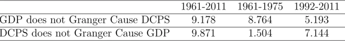
First, we compute the Granger causality tests . For the entire period studied and also

for the 1992-2011 sub-period GDP seems to be helpful in predicting DCPS and vice-versa.

However, in the 1961-1975 sub-period GDP is said to be Granger-caused by DCPS but the

opposite does not occur. The results are shown in the table 1.

Table 1: Granger causality tests F-statistics by sub-periods (1961-2011)

1961-2011 1961-1975 1992-2011

GDP does not Granger Cause DCPS

9.178

8.764

5.193

DCPS does not Granger Cause GDP

9.871

1.504

7.144

When considering the entire period, both OLS and DOLS estimates (equations 2 to

5) show that GDP explains DCPS and vice-versa. The results are presented in table 2 .

However, when analyzing the two sub-periods closely the results are different. In the first

sub-period (1961-1975) both variables are non-stationary and cointegrated, which means

they have to be analysed in a Vector Error Correction (VEC) model, as expressed in the

following equations 6 and 7:

∆GDPt=βGDP,0+β_GDP,GDP,1∆GDP_t−1+β_{GDP,DCP S,}1∆DCP S_t−1+

+λGDP(GDPt−1−α0−α1DCP St−1) +ν GDP t

∆DCP St=βDCP S,0+β_{DCP S,GDP,}1∆GDP_t−1+β_{DCP S,DCP S,}1∆DCP S_t−1+

+λDCP S(GDPt−1−α0−α1DCP St−1) +ν DCP S t

(7)

where ∆GDP and ∆DCP S in first differences, respectively, λGDP and λDCP S are the

error-correction coefficients, νGDP

t and νtDCP S are the error terms, and the expressions in

parenthesis are the cointegrating vector between the variables. The results of equations

(6) and (7) are presented in table 3.

Table 2: Estimation results for DCPS and GDP between 1961-2011 and 1992-2011 periods.

GDP DCPS

1961-2011 1961-2011

OLS DOLS OLS DOLS

DCPS 0.053*** 0.079*** GDP 11.240*** 12.002*** (0.006) (0.007) (1.329) (2.769)

R2

0.5983 0.928 0.598 0.800

Obs. 46 45 50 46

1992-2011 1992-2011

OLS DOLS OLS DOLS

DCPS 0.002*** -0.000** GDP 281.298*** 19.095** (0.000) (0.000) (13.876) (8.137)

R2

0.653 0.725 0.958 0.709

Obs. 20 18 20 18

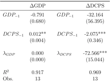
Table 3: Estination results for VEC model.

∆GDP ∆DCPS

GDP₋1 -0.791 GDP₋1 -32.164

(0.680) (56.395)

DCP S₋1 0.012** DCP S₋1 -2.075***

(0.004) (0.346)

λGDP 0.000 λDCP S -72.566*** (0.000) (15.044)

R2

0.917 0.969

Obs. 13 13

*, ** and *** represent statistical significance at levels of 10%, 5% and 1%, respectively. Standard errors are in parenthesis.

The results from equation (6) show the existence of short-run causality coming from

DCPS to GDP but the ones from equation (7) do not show the existence of short-run

causality coming from GDP to DCPS. It may be explained by the fact that throughout

this period DCPS growth had an erratic behaviour that did not match the GDP growth.

It is clear how DCPS grew significantly particularly in 1969, 1973 and 1975 while GDP did

not. In fact, for instance, in 1975 DCPS grew 36% while GDP only grew 1%. In addiction,

from the result for error-correction coefficients of equation (7), we obtain a significant

negative result for λDCP S meaning that there is a long-run causality from GDP to DCPS,

i.e. GDP causes DCPS in the long-run. In short, GDP causes DCPS in the long-run but

not in the short-run.

The sub-period between 1992 and 2011 also reveals interesting results. Even tough the

OLS method shows that GDP and DCPS explain each other, the DOLS approach does

not show that GDP explains DCPS. And since DOLS is considered a more robust and

improved method, this final result will be taken seriously into account because it may be

It must be noticed that the Granger Causality Test results seem to contradict the

OLS and DOLS results. In the first sub-period, GDP does not granger-cause DCPS and

the VEC model actually does not show short-run causality coming from GDP to DCPS.

However, in the second sub-period where GDP and DCPS seem to be helpful in predicting

each other, DOLS shows that GDP does not explain DCPS. As mentioned previously, the

Granger Causality Test aim was only to give a hint about the ability of each variable to

predict each other. Despite of this possible contradiction, it is important to consider the

limitations of econometric analysis since it is impossible to capture all the effects of all

variables. A completely correct and flawless analysis is simply impossible.

Results analysis

From the results presented in the previous section, two main conclusions arise.

First, similar to the Irish case (see Kelly et al. (2011)), for Portugal the BCBS

ap-proach does not appear to be the most suitable. Portugal clearly has two outstandingly

different periods (1961-1975 and 1992-2011) that must be taken into account separately.

Even though the results considering the entire period seem well-behaved it disguises the

astonishing evolution this ratio has been having. As explained in section 3, the BCBS

approach apparently only works for economies which did not had a rapid credit build-up

and our results seem to corroborate this idea. The DCPS-to-GDP ratio is an indicator of

financial instability but the approach to analyse it should be taken into account carefully

in order to produce the best results. As a small and open economy that had a huge credit

build-up, Portugal should definitely pay attention to it in order to track the evolution of

households’ indebtedness and its own financial stability.

Second, the DOLS results for the second sub-period showing that GDP does not explain

DCPS may suggest a break of the link between deposits and credit. Traditionally, banks

has always been this link that had kept the banking system sound and stable. However, the

data for GDP and DCPS variables from WDI evidence some sub-periods where the DCPS

growth rate was significantly higher than the GDP growth rate. Assuming that savings

are related to a country’s economic performance and taking into account that Portugal’s

GDP did not grew significantly in the past two decades, apparently credit growth was not

accompanied by a growth in savings, especially from 1990’s decade (Banco de Portugal

(2004)).

From approximately the 1990 decade that traditional banking conduct was not the

case for the Portuguese banking sector. Due to the lack of domestic resources and a strong

credit growth fuelled by households’ housing demand, banks had to resort to alternative

forms to finance credit, such as the international financial markets. Banks realized that

there was no longer the obligation to only grant credit with respect to deposits since they

had access to an almost limitless pool of funds at a low interest rate that allowed them to

do business differently.

Conclusions

This paper analyses the reasons of the Portuguese households’ indebtedness. Since the

2008’s financial crisis it has been a growing concern for authorities to be provided with the

so-called early warning indicators in order to be able to take prudent actions when facing

financial distress. The BCBS suggests using the HP-Filter to determine the Private Sector

credit-to-GDP gap i.e., the difference between the credit-to-GDP ratio and its own

long-term trend, and recommends it as a common starting point for authorities to delong-termine

whether there is an excessive credit growth or not.

This approach is not bullet-proof and some authors have shown that it is not the most

reached the same conclusion for the case of Ireland, a small and open economy. Due to the

similarities with Portugal, this paper uses Kelly et al (2011) empirical analysis to determine

if the BCBS approach is the most appropriate or not.

With World Development Indicators data of the DCPS-to-GDP ratio from 1961 to 2011,

a two-state Markov Switching model was constructed to explore the structural breaks the

ratio may have and the periods where long-run estimates could be made. There were

two major structural breaks that showed two important sub-periods: 1961 to 1975 and

1992 to 2011. The long-run relationship between DCPS and GDP was analyzed in these

sub-periods as well in the entire period using OLS and DOLS methods.

There are two main conclusions. The first one is that BCBS approach is not the most

suitable for the case of Portugal because it disguises the existence of two outstandingly

different periods, particularly the second one.

The second main conclusion is that GDP does not explain DCPS from 1992 to 2011,

which probably indicates that the link between deposits and credit has been broken in

this sub-period. Banks started to get financing in international financial markets in order

to satisfy the particularly strong households’ housing demand which, in fact, was partly

encouraged by banks with attractive mortgages even for households with a more modest

income. Even though the banking sector had an irresponsible conduct, it was not stopped or

prevented by Banco de Portugal who assumed a passive attitude towards the development

of the situation, although perfectly aware of it.

The evolution of Portugal’s DCPS-to-GDP ratio was a considerably loudearly warning

indicator that was not seriously taken into account by authorities. It encouraged the

Por-tuguese bank’s daring behaviour during the 1990’s and beginning of the 2000’s and fuelled

References

Banco de Portugal (2004). Financial Stability Report. Technical report, Banco de Portugal.

Castro, G. L. (2006). Consumption, disposable income and liquidity constraints. Economic

bulletin, Banco de Portugal.

Costa, S. (2012). Households’ default probability: an analysis based on the results of the

HFCS. Financial stability report, Banco de Portugal.

Costa, S. and Farinha, L. (2012). Households’ indebtedness: a microeconomic analysis

based on the results of the households’ financial and consumption survey. Financial

stability report, Banco de Portugal.

Drehmann, M. (2013). Total credit as an early warning indicator for systemic banking

crises. Bis quarterly review, Bank for International Settlements.

Drehmann, M., Borio, C., Gambacorta, L., Jim´enez, G., and Trucharte, C. (2010).

Coun-tercyclical capital buffers: exploring options. BIS Working Papers 317, Bank for

Inter-national Settlements.

Drehmann, M., Borio, C., and Tsatsaronis, K. (2011). Anchoring countercyclical capital

buffers: the role of credit aggregates . BIS Working Papers 355, Bank for International

Settlements.

Farinha, L. (2007). Indebtedness of Portuguese households: recent evidence based on the

household wealth survey 2006-2007. Economic bulletin and financial stability report

articles, Banco de Portugal.

Farinha, L. and Noorali, S. (2004). Indebtedness and wealth of portuguese households.

Gersl, A. and Seidler, J. (2011). Excessive Credit Growth as an Indicator of Financial

(In)Stability and its Use in Macroprudential Policy. CNB Financial Stability Report

2010/2011, Czech National Bank, Research Department.

Giese, J., Andersen, H., Bush, O., Castro, C., Farag, M., and Kapadia, S. (2014). The

credit-to-gdp gap and complementary indicators for macroprudential policy: Evidence

from the uk. International Journal of Finance & Economics, 19(1):25–47.

Hansen, N.-J. H. and Sulla, O. (2013). Credit Growth in Latin America; Financial

Devel-opment or Credit Boom? IMF Working Papers 13/106, International Monetary Fund.

Jord`a, O., Schularick, M., and Taylor, A. M. (2010). Financial Crises, Credit Booms, and

External Imbalances: 140 Years of Lessons. Working Paper 16567, National Bureau of

Economic Research.

Kelly, R., McQuinn, K., and Stuart, R. (2011). Exploring the Steady-State Relationship

between Credit and GDP for a Small Open Economy - The Case of Ireland. Research

Technical Papers 1/RT/11, Central Bank of Ireland.

Lopes, J. S. (1982). IMF conditionality in the stand-by arrangement with Portugal of 1978.

Estudos de Economia, III(2):141–166.

Pinto, A. (1983). A economia portuguesa e os acordos de estabiliza¸c˜ao econ´omica com o

Fundo Monet´ario Internacional. Economia, VII(3):555–596.

Rubaszek, M. and Serwa, D. (2014). Determinants of credit to households: An approach

using the life-cycle model. Economic Systems, 38(4):572 – 587.

Shin, H. S. (2013). Procyclicality and the Search for Early Warning Indicators. IMF

Stock, J. H. and Watson, M. W. (1993). A Simple Estimator of Cointegrating Vectors in