Fiscal policy sustainability: some unpleasant European evidence

(1)

evidence

António Afonso

Department of Economics,

Instituto Superior de Economia e Gestão, Universidade Técnica de Lisboa,

R. Miguel Lúpi, 20, 1249-078 Lisbon,

Portugal

Tel.: +351 21 392 2807 Fax: +351 21 396 6407 e-mail: aafonso@iseg.utl.pt

This version: August 2000

Abstract

The sustainability of fiscal deficits has been receiving increasing attention from economists. The issue is paramount for the newly formed Euro area and this is one of the motivations of the paper. In order to assess the sustainability of budget deficits in the Euro area, stationarity tests for the stock of public debt and co-integration tests between public expenditures and public revenues are performed for the Euro countries for the 1968-1997 period. The empirical results allow us to conclude that fiscal policy may not be sustainable for most countries with the possible exceptions of Germany, Austria and the Netherlands.

Keywords: Deficit finance; inter-temporal budget constraint; fiscal policy sustainability; Euro area

JEL classification: E60; H62; H63

*

This paper is part of the research project for the author’s Ph.D. thesis. The author acknowledges comments from Jorge Santos, participants in the 2000 Annual Meeting of the European Public Choice Society Conference in Siena, April 2000, participants in the 5th

(2)

"…the government's intertemporal budget constraint is a constraint on the government's instruments that must be satisfied for all admissible values of the economy-wide endogenous variables," Buiter (1999).

1 - Introduction

In recent years several developed countries have been facing significant fiscal

deficits. The government's ability to cope with fiscal deficits has been receiving

increasing attention from economists. Fiscal sustainability seems quite a recurrent topic

that both individual countries and international organisations dwell upon with some

regularity.1 The issue is paramount for the newly formed Euro area and this is one of the

motivations of this paper.

Already quite a lot of literature has studied the issue of fiscal policy

sustainability and empirically tested the present value borrowing constraint. Examples

of such a growing literature are for instance Hamilton and Flavin (1986), Trehan and

Walsh (1988, 1991), Kremers (1988, 1989), Wilcox (1989), Hakkio and Rush (1991),

Tanner and Liu (1994), Quintos (1995), Haug (1991, 1995), Ahmed and Rogers (1995),

Uctum and Wickens (1997), Crowder (1997), Payne (1997) and Artis and Marcelino

(1998). The main tools used to analyse the sustainability of budget deficits seem to be

stationarity tests for the stock of public debt and co-integration tests between

government expenditures and government revenues.

The paper is organised as follows: the next section offers some considerations on

the arithmetic of budget deficits; section three reviews the theoretical framework of

budget deficits sustainability and the approaches used in the literature to validate the

sustainability of fiscal policy. Stationarity tests and co-integration test results, between

government expenditures and government revenues for the EU-15 countries, are the

main focus of section four. Section five is a conclusion.

(3)

2 - The arithmetic of budget deficits and public debt

Previous to the sustainability issue, a review of the fiscal deficit arithmetic

seems to be in order, to help set the theoretic framework for the subsequent

sustainability analysis.

The government borrowing constraint for period t may be written with the

following dynamic equation

(

1

)

1

) 1

( + ₋ + − − − ₋

= t t t t t t

t i B G R M M

B (1)

were the variables are defined as follows: G - government expenditures, excluding interest payments; R - government revenues; B - public debt; i - nominal interest rate, implicit in public debt; M - nominal monetary base. It is possible to simplify the notation namely by suppressing the time indexes,

M iB R G

B = − + −∆

∆ . (2)

In order to analyse the evolution of the debt-to-GDP ratio it is necessary to

compute the total derivative of B/Y:

d B

Y YdB

B Y dY



  = + −  1

2 (3)

or, with a notation similar to the one in equation (2),

∆ B ∆ ∆

Y

B Y

Y Y



  = − . (4)

Defining b = B/Y and n = ∆Y/Y, the preceding equation is also identical to

∆b ∆B Y bn

(4)

Substituting (2) in (5) gives,

bn Y

M Y

R iB G

b= + − −∆ −

∆ (6)

and after defining g = G/Y and ρ = R/Y,

bn Y

M ib

g

b= + − −∆ −

∆ ρ . (7)

Assuming λ as the growth rate of monetary base, λ = ∆Μ/Μ, and defining also

m = M/Y,

∆M M

M

Y = λm, (8)

and using equations (9) and (8),

bn m ib

g

b= + − − −

∆ ρ λ , (9)

it is then possible to write the long-run budget constraint, which means that ∆b=0, as

m ib

g

nb= + −ρ −λ , (10)

in words, the long-run deficit will be proportional to the level of public debt and the

economy nominal growth rate is the proportionality factor.

The previous equation is useful to perform some simple and illustrating

calculations. Assume that the debt-to-GDP ratio is stable at 60 per cent and that the

economy nominal growth rate is 4,5 per cent in annual terms. Then the government will

end up to incur in an annual deficit of 2,7 per cent of GDP (deficit = 4,5×0,6 = 2,7 per

(5)

Using the Fisher relation for the interest rate, r = i - π and for the economy growth rate, n = y + π, we have

) (r y

b m g

b= − − + −

∆ ρ λ , (11)

a formulation identical to the one present throughout the literature (see for instance

Buiter (1985) and Spaventa (1987)).

With equation (11) it is possible to confirm the explosive characteristic of the

debt-to-GDP ratio when r > y. In fact, the debt-to-GDP ratio increases when the real interest rate is above the real GDP growth rate and when the government has primary

deficits. Finally, assuming again that the debt-to-GDP stabilises at a certain level, it is

possible to solve equation (11) for b, which gives,

) /( )

( g m r y

b= ρ− +λ − . (12)

The budget constraint in equation (9) is really a differential equation in a

continuous time scenario, that is (forgetting for simplicity money financing),

t t

t d nb

b. = − (13)

where dt is the budget deficit as a percentage of GDP in period t. With the hypothesis of balanced budgets, dt = 0, we have

t

t nb

b. =− . (14)

The solution of the above differential equation may be written as

nt

t Ce

b ₌ − (15)

and, in the long-run, this expression approximates zero since lim

[

]

= 0. ∞

→ −

nt

(6)

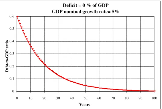
Figure 1 illustrates the evolution of the debt-to-GDP ratio when there is a

balanced budget and the annual nominal growth rate of GDP is 5 per cent, and it is

possible to see that assuming a positive growth rate one gets a declining debt-to-GDP

ratio.

[Insert Figure 1 about here]

Some calculations where also made in order to understand the possibility of

several combinations of government expenditures and government revenues together

with different debt-to-GDP ratios. A real GDP growth rate of 2,5 per cent was used,

also with an inflation rate of 2 per cent along with a level of 40 per cent of GDP for

government revenues and expenses.

Three alternative hypotheses for the real interest rate were also used. The

calculations were made as follows: first, the deficit is computed for the several values of

the debt-to-GDP ratio, then the interest expenses are calculated and finally the

government revenues (expenditures) are derived holding the government expenditures

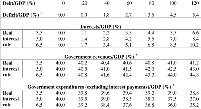
(revenues) constant. Table 1 presents the results of the simulations.

[Insert Table 1 about here]

Suppose for instance that government expenditures are 40 per cent of GDP and

that government revenues must adjust in order for the long run budget constraint to be

satisfied. Since we have r > y, the bigger the debt-to-GDP ratio the bigger the necessary increase of public receipts.

Also, the bigger the difference between the real interest rate and the real growth

rate, the higher should be the level of government revenues as a percentage of GDP.

Another conclusion is that as the debt-to-GDP ratio increases, the growth rate of

government revenues is smaller than the growth rate of the public debt interests. As a

matter of fact, it is important to notice that the effective cost of financing an additional

(7)

unit is financed through new debt, the stock being increased at the same rate of the real

GDP growth rate.

Identical calculations may be carried out in order to show that higher levels of

deficits and public debt may be consistent with a reduction of government expenditures,

as an alternative to the increase of government revenues. In this case, a higher public

indebtedness is associated with a decrease of government expenditures, at a lower rate

than the increase of the public debt interests. Observe nevertheless that all these

calculations are simple static exercises, not taking into account for instance that the

level of the stock of public debt may have some influences on real GDP growth rate, on

the real interest rate and on inflation.2

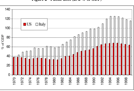
The consequences of choosing different fiscal policies may also be exemplified

by looking at the public debt paths of the US and Italy. In 1970 the debt-to-GDP ratio

was 38 per cent in both countries as can be seen in Figure 2. However, during the period

1970-1990 Italy had an average public deficit of 9 per cent of GDP while the US had an

average deficit of only 2,2 per cent of GDP. The result was that in 1999 public debt was

116 per cent and 64 per cent of GDP respectively in Italy and in the US. Even if we take

into account the different GDP growth rates in the two countries, adding up successive

and significant budget deficits in Italy had a clearly identifiable impact on government

debt.

3 - The sustainability issue

The sustainability of fiscal policy is sometimes confused with the financial

solvability of the government. In practice however, what the empirical literature ends up

testing is whether both public expenditures and government revenues may continue to

display in the future their historical growth patterns. This seems really to be the issue

here, not so much a question of solvability.

2 _{A macroeconomic model would be necessary for that purpose. See for instance the paper of}

(8)

If a given fiscal policy turns out to be unsustainable, it has to change in order to

guarantee that the future primary balances are consistent with the budget constraint.3

Theoretically any value for the budget deficit would be possible if the government could

rise its liabilities without limit. Obviously, that is impossible since the government is

faced with the present value of its own budget constraint.

In the beginning of the 20s, when writing about the public debt problem faced by

France, Keynes (1923) alerted to the need for the French government to conduct a

sustainable fiscal policy in order to satisfy its budget constraint. Keynes stated that the

absence of sustainability would be evident when

"the State's contractual liabilities (…) have reached an excessive proportion of the

national income" (p. 54).

In modern terms, sustainability is challenged when the debt-to-GDP ratio

reaches an excessive value. There is a problem of sustainability when the government

revenues are not enough to keep on financing the costs associated to new issuance of

public debt or, in Keynes's words, when

"it has become clear that the claims of the bond-holders are more than the tax payers

can support" (p. 55).

At that stage the government will have to take measures that allow regaining the

sustainability of fiscal policy, that is the State

"must come in due course to some compromise between increasing taxation, and

diminishing expenditure, and reducing what (…) [it] owe[s]" (p. 59).

Blanchard et al (1990) present as a definition of sustainable fiscal policy one that allows, in the short term, that the debt-to-GDP ratio returns to its original level after

some excessive variation. Put another way, for a fiscal policy to be sustainable, after

(9)

having accumulated debt in the past, the government must run primary surpluses in the

future.

It is worthwhile noticing that the hypothesis of fiscal policy sustainability is

related to the condition that the trajectory of the main macroeconomic variables is not

affected by the choice between the issuance of public debt or the increase in taxation.

Under such conditions, it would therefore be irrelevant how the deficits are financed,

implying also the validation of the Ricardian Equivalence issue.4

In short, two alternative definitions for fiscal policy or budget deficit

sustainability may be presented, to be analytically derived on the next section:

i) the value of public current debt must be equal to the sum of future primary

surpluses;

ii) the present value of public debt must approach zero in infinity.

3.1 - The present value of the budget constraint

The government budget constraint is naturally the starting point to derive the

present value of the budget constraint. Writing once more the budget constraint, now in

real terms, a more adequate presentation for posterior analytical developments,5 we

have

t t t t

t r B R B

G +(1+ ) ₋1 = + (16)

with G - government expenditures, in real terms, excluding interest payments; R -government revenues, in real terms; B - public debt in real terms; r - real interest rate.

4

Caporale (1995) mentions this question. Afonso (1999) presents some empirical results on the feasibility of Ricardian Equivalence in the Euro area.

5 _{Note that sometimes in the literature, for the validation of theoretical results, the real interest}

(10)

Rewriting equation (16) for periods t+1, t+2, t+3,..., and recursively solving that

equation leads to the following intertemporal budget constraint

∑

∏

∞ = = + + = + + + + ∞ → + + − = 1 1 1 ) 1 ( lim ) 1 ( s s

j t j

s t s j j t s t s t t r B s r G R

B . (17)

When the second term from the right-hand side of equation (17) is zero, then the

present value of the existing stock of public debt will be identical to the present value of

future primary surpluses. Also, when the limit term is zero, this means that in the long

run the government will have to stop using Ponzi games to finance fiscal deficits.

Equation (17) is not appropriate for empirical testing. It is therefore adequate to

make several algebraic modifications to equation (16). Assuming that real interest rate

is stationary, with mean r, and defining

1

)

( − ₋

+

= t t t

t G r r B

E , (18)

it is possible to obtain the following expression

∑

∞ = + + + + + − = ₊ − + _→_∞ ₊ 0 1 1 1 ) 1 ( lim ) ( ) 1 ( 1 s s s t s t s t s t r B s E R r

B . (19)

A sustainable fiscal policy should assure that the present value of the stock of

public debt goes to zero in infinity, which means taking into account the following

transversality condition, constraining the debt to grow no faster than the interest rate,

0 ) 1 ( lim 1 = + ∞

→ + s+

s t

r B

s , (20)

or, in other words, it means to impose the absence of Ponzi games and the fulfilment of

the intertemporal budget constraint.6 By imposing the transversality condition, the

(11)

government will have to present in the future primary surpluses whose present value

add up to the current value of the stock of public debt. Still another way of putting it is

that public debt in real terms cannot increase indefinitely at a growth rate beyond real

interest rate.7

Let us now proceed with the derivation of the solvency condition, with all the

variables defined as a percentage of GDP. For instance Hakkio and Rush (1991, pp.

430) support that an analysis based on ratios is more appropriated for growing

economies:

"(...) in addition to examining revenue and spending directly, we also use normalize

these variables using real GNP and population. This is an important extension beyond

previous work since McCallum [1984], among others, deems these ratios - per capita

spending and revenue, and spending and revenue as a fraction of GNP - as more

pertinent for a growing economy."

The present value of the borrowing constraint, with the variables expressed as a

percentage of GDP, and neglecting for presentation purposes seigniorage revenues, is

written as t t t t t t t t t t Y R Y G Y B y r Y B − + + + = − − 1 1 ) 1 ( ) 1 (

. (21)

By means of a similar procedure to the one we obtained equation (19), where

real interest rate is assumed stationary, with mean r, and considering also a constant real economic growth rate, the budget constraint is then given by

[

]

( 1)

0 ) 1 ( 1 1 1 lim 1 1 + + + + ∞ = + −       + + ∞ → + −       + + =

∑

s s t s t s t s s t r y b s e r y

b ρ (22)

with bt = Bt/Yt, et = Et/Yt and ρt = Rt/Yt.

7 _{See Joines (1991). McCallum (1984) discusses if this is a necessary condition to obtain an}

(12)

When r > y, a characteristic of a dynamically efficient economy,8 it is necessary to introduce a solvency condition in order to bound public debt growth. This implies

that the growth rate of the debt-to-GDP ratio should be less than the factor

) 1 ( 1 1 +       + + s r y ,

being the transversality condition given by

0 1

1

lim ( 1)

=       + + ∞ → + + s s t r y b

s . (23)

Using the budget constraint, equation (22), and the solvency condition, equation

(23), we get

[

t s t s

]

s

t e

r y

b ∞ ₊ ₊

= + −  −      + +

=

∑

ρ

0 ) 1 ( 1 1 1 , (24)

the by now familiar result that fiscal policy will be sustainable if the present value of the

future stream of primary surpluses, as a percentage of GDP, matches the "inherited"

stock of public debt.9

3.2 - Assessment of the sustainability of public deficits

Returning to equation (19), it is now possible to present analytically two

complementary definitions of sustainability, which set the background for most

empirical testing:

i) the value of public current debt must be equal to the sum of future primary surpluses

∑

∞

= + + +

− = ₊ −

0

1

1 ( )

) 1 ( 1 s s t s t s

t R E

r

B , (25)

8_{See for instance Abel et al (1989) and Frisch (1995).}

9 _{According to Buiter (1999), the intertemporal government budget constraint should be}

(13)

ii) the present value of public debt must approach zero in infinity

0 ) 1 ( lim

1 =

+ ∞

→ + s+

s t

r B

s . (26)

The literature exhibits generically two main approaches to test the sustainability

hypothesis: tests similar to the one suggested by Trehan e Walsh (1991) and tests like

the one credited to Hakkio e Rush (1991).

Trehan and Walsh (1991)

In order to test empirically the absence of Ponzi games, the authors propose to

test the stationarity of the first difference of the stock of public debt. It is therefore

necessary for (1-L)Bt to be a stationary process, where L is the lag operator.10 To test

for the stationarity of the (1-L)Bt series, it is possible to use the unit root tests developed

by Dickey and Fuller (1979, 1981). Trehan and Walsh (1991) assume also that the real

interest rate is not constant, and that a stochastic process may represent it.11 The

stationarity tests for (1-L)Bt are conducted using

∑

= −

− + − +

− + + =

− m

i

t i t i

t

t t L B L B u

B L

1

2 1

0 2

) 1 ( )

1 ( )

1

( λ α β β , (27)

with the null hypothesis given by H0 :β0 =0, H1:β0 <0.

If the null hypothesis is rejected, then the process (1-L)Bt is stationary and the

sustainability hypothesis may be accepted. If on the other hand the null is not rejected,

then the process (1-L)Bt may only be stationary in the first differences, which can mean

sustainability problems. As observed by Trehan and Walsh (1991), the stationarity of

the variation of the stock of public debt is a sufficient condition, and stationarity

10_{For instance Sawada (1994) also uses this approach to study the sustainability of external debt}

in several Southeast Asia and South America countries.

11_{Hénin (1997), supports that in a deterministic context sustainability appears as a stability}

(14)

rejection does not necessarily imply the absence of sustainability of the government

accounts.12

Hakkio and Rush (1991)

Hakkio and Rush (1991) initially developed the empirical approach of the

sustainability of fiscal policy through co-integration tests. The implicit hypothesis

concerning the real interest rate, with mean r, is also stationarity. The intertemporal budget constraint, equation (17), may also be written as13

[

]

1

0 1 1 1 1 ) 1 ( lim ) 1 ( 1 + + ∞ = − + + + −+ −+ − − = ₊ ∆ −∆ −∆ ∆ + ∆ +_→_∞ ₊

+

∑

t s_s

s s t s t s t s t s t s t t t t r B B r B r G R r R B r G , (28)

and using once more the auxiliary variable E_t =G_t +(r_t −r)B_t₋₁, we arrive to

∑

∞ = + + + + − − − = ₊ ∆ −∆ + _→_∞ ₊ + 0 1 1 1 ) 1 ( lim ) ( ) 1 ( 1 s s s t s t s t s t t t t r B s E R r R B r

G . (29)

With the no-Ponzi game condition, 0 ) 1 ( lim 1 = + ∞

→ + s+

s t

r B

s , and with the

additional definition

1

− + = t t t

t G rB

GG , (30)

it is possible to derive

1 0 1 ) 1 ( lim ) ( ) 1 ( 1 + + ∞ = − + + →∞ + + ∆ − ∆ + =

−

∑

t s_s

s s t s t s t t r B s E R r R

GG , (31)

12_{See Trehan and Walsh (1991).} 13

(15)

where GGt and Rt must be co-integrated variables of order one for their first differences to be stationary.

Assuming that R and E are non-stationary variables, and that the first differences are stationary variables, implying that the series R and E in level are I(1), then for equation (31) to hold, the left-hand side of equation (31), will also have to be stationary.

If it is possible to conclude that GG and R are integrated of order 1, these two variables should be co-integrated with co-integration vector (1, -1), for the left-hand side of

equation (31) to be stationary.

The usual procedure to assess the sustainability of the intertemporal government

budget constraint involves testing the following co-integration regression14

t t

t a bGG u

R = + + . (32)

The null hypothesis of no co-integration, that is, the hypothesis that the two I(1)

variables are not cointegrated, is rejected if a high-test statistic is obtained implying that

one should accept the alternative hypothesis of co-integration. For that result to hold

true, the series of the residuals ut must be stationary, and should not display a unit root.15

The empirical results may allow establishing several conclusions concerning the

sustainability of the intertemporal budget constraint:

i) when there is no co-integration the fiscal deficit is not sustainable;

ii) when there is co-integration with b=1, the deficit is sustainable,

14 _{In short, two variables are said to be co-integrated when each variable by itself is not}

stationary, but there is a linear combination of the two variables which is stationary, and it may exist a value of a and b such that R_t −bGG_t −a=u_t is stationary. If the two variables are cointegrated, they cannot deviate from the co-integration relation beyond constant fluctuations bands, since ut has a constant variance.

15 _{Fève and Hénin (1998) propose an alternative test for unit roots, the test FADF (Feedback}

(16)

iii) when there is co-integration, with b < 1, government expenditures are

growing faster than government revenues, and the deficit may not be

sustainable.16

Hakkio and Rush (1991) demonstrate also that if GG and R are non stationary variables in level, the condition 0 < b < 1 is a sufficient condition for the budget

constraint to be obeyed. However, when revenues and expenses are expressed as a

percentage of GDP or in per capita terms, it is necessary to have b = 1 in order for the

trajectory of the debt-to-GDP not to diverge in an infinite horizon.17

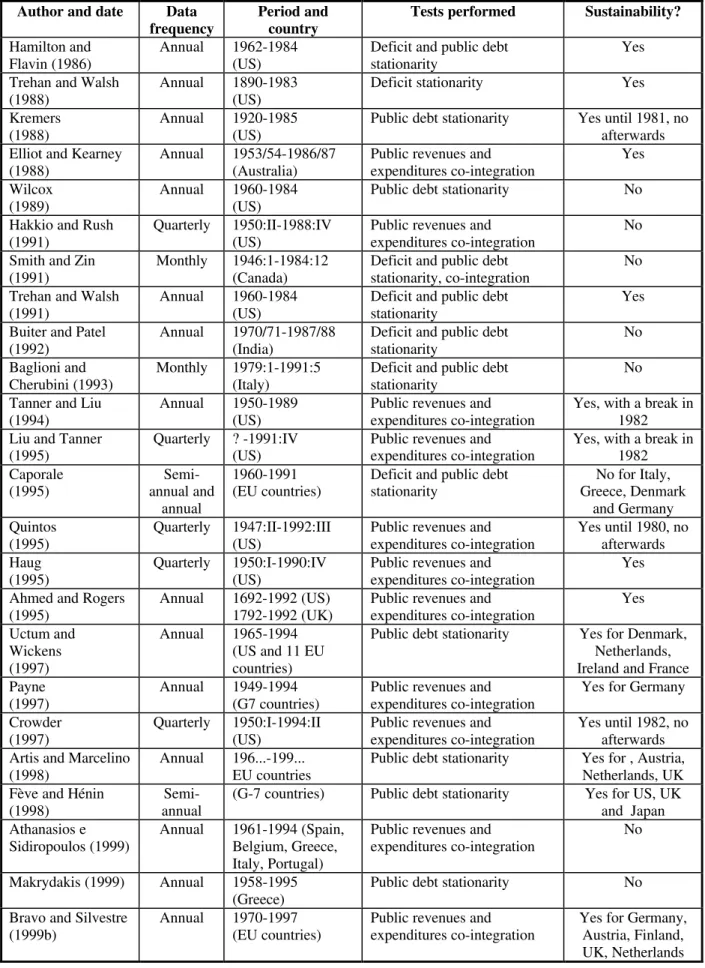
Before proceeding it seems adequate to close the present section summarising

the empirical findings of several other papers, concerning the sustainability issue. Table

2 sums up the conclusions of some of those papers.

4 - Fiscal policy sustainability in the EU-1 5 area

4.1 - Some historical facts

A brief characterisation of the debt and fiscal burden on GDP, for the EU

countries, seems appropriate before performing the empirical testing of the

sustainability hypothesis.

Between the end of the 60s and the end of the 90s there was an increasing trend

of the debt-to-GDP ratio for most countries throughout the period. For instance, public

debt rose in Italy from 38 per cent of GDP in 1970 to 118 per cent of GDP in 1998. In

Germany the debt-to-GDP ratio was 18,6 per cent in 1970 and went beyond the 60 per

cent level in the 1996. Also in Portugal, public debt progressed from 15,4 per cent of

GDP in 1974 to 60 per cent in 1998.

16_{Concerning this cointegration analysis approach Bohn (1991, 1995) argues that a sustainable}

fiscal policy in a certain environment, may bacome unsustainable under uncertainty.

17 _{Quintos (1995), Ahmed and Rogers (1995) and Bergman (1998) discuss the necessary}

(17)

The highest reported debt-to-GDP ratios are in Italy and Belgium (the country

with the highest ratio in the period from 1970 to 1998: 135,2 per cent in 1993), around

118 per cent of GDP in 1998, and their high debt service payments induce substantial

budget deficits despite primary budget surpluses. A reversal of that general trend is

observable only in the end of the 90s, as the countries naturally tried to fulfil the

Maastricht criterion on the debt-to-GDP ratio.

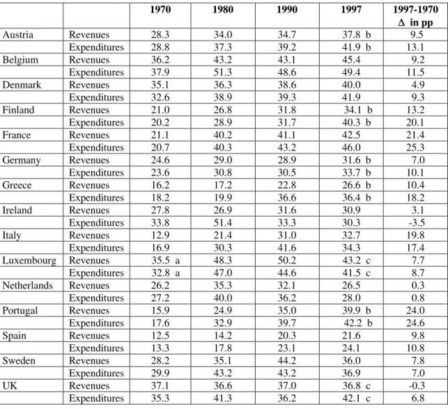
Concerning public expenditures and public revenues, Table 3 presents those

items as a percentage of GDP for each country. The main conclusion is that the burden

of public expenditures and revenues on GDP has increased since the 70s for almost

every country. Also another obvious fact is that for most countries, the ratio of

government expenditures to GDP exhibited a higher growth rate than the ratio of

government revenues to GDP. This conclusion holds for all countries except for Ireland,

Italy and Sweden.

For instance in Portugal, the ratio of government revenues and expenditures to

GDP was respectively 15,9 and 17,6 per cent in 1970, while those ratios where at 39,9

and 42,2 per cent in 1996. The case of Ireland is quite remarkable since the ratio of

public expenditures to GDP actually decreased around 3,5 percentage points between

1970 and 1997, and one must bear in mind the high real GDP growth rates of Ireland

during the 90s.

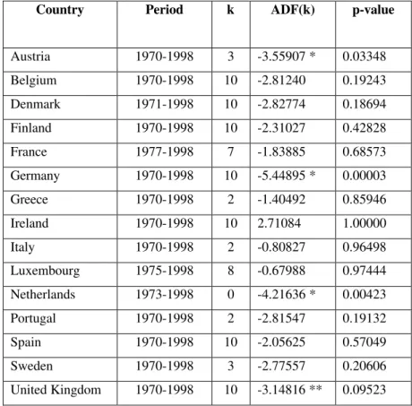
4.2 - Public debt stationarity tests

The focus of this section is the study of public debt stationarity for each of the

EU-15 countries. Augmented Dickey-Fuller tests are used in the attempt to validate the

sufficient sustainability condition, and the variable used is the stock of public debt.

Table 4 gives the stationarity tests results for the first difference of the stock of public

(18)

The results show that the process (1-L)Bt is stationary (at a 5 per cent level), the

series of the first difference of public debt are I(0), for Austria, Germany and

Netherlands. In other words, the solvency condition would be satisfied for only those

three countries. For the remaining countries, the rejection of the stationarity hypothesis

does not mean, as already noticed above, the insolvency of public accounts since the

above hypothesis is only a sufficient condition and not a necessary one. For the United

Kingdom the stationarity hypothesis could only be accepted at a significance level of 10

per cent.

4.3 - Co-integration between government revenues and expenditures

In this section, fiscal sustainability in the EU-15 countries is studied by testing

the existence of co-integration between government expenditures and revenues. Once

more the variables are used in real terms, at 1990 prices, the data sources being given in

the Appendix.

The first step is to test the existence of a unit root for all the expenditures and

revenues series in level.18 The results for the augmented Dickey-Fuller tests (not

presented in the interest of brevity) allow us to conclude that almost all series are not

stationary in level. It was therefore necessary to test for the stationarity of the first

differences. In general, it is possible to accept the stationarity of the first differences of

the government expenditures and revenues series. One can then accept that the first

differences of the original series, in real terms, are I(0), which means that the series in

level are I(1). For some countries it is not possible however to accept the stationarity of

the first differences of the original series. This is for instance the case of Germany,

where expenditures are not I(1), and Luxembourg where revenues are not I(1), at the 5

per cent level. For Ireland and the United Kingdom neither expenditures nor revenues

are I(1) at the 10 per cent level.

(19)

After assessing the stationarity of the government series, it is now possible to

conduct co-integration tests between the revenues and the expenditures, for the

countries where those variables are integrated of order 1.19 The test results for

integration (not presented for space saving), allow us to reject the hypothesis of

co-integration between government expenditures and government revenues for all

countries.20 Therefore, with the series in level, it is not possible to accept the hypothesis

of fiscal sustainability for those countries, for the period under analysis.

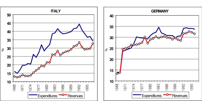
In a second stage the government expenditures and revenues were taken as a

percentage of GDP, still in real terms. Visual inspection may give already a clue as can

be seen by the examples of Figure 3, which depicts government expenditures and

revenues, as a percentage of GDP, for Italy and Germany.

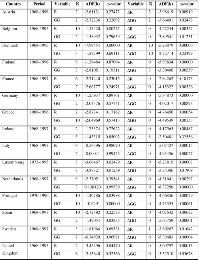
Unit root tests were then performed for the government expenditures and

revenues as a percentage of GDP, the results being presented in Table 5. It is interesting

to notice that now stationarity is the main conclusion, even if there are some exceptions.

It is not possible to accept that both variables are I(1) in Denmark, where expenditures

are not I(1); in France revenues are not I(1) and in Ireland where expenditures are not

I(1), at least at 10 per cent level.

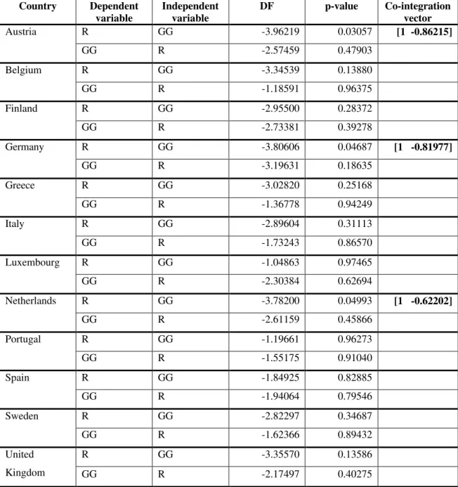
The co-integration tests, for the countries were this procedure is now

appropriate, were then performed with the government revenues and expenditures as a

percentage of GDP. Obviously, Denmark, Ireland and France were excluded from these

tests. The results are presented in Table 6.

19

Cointegration tests for non-stationary variables, as proposed by Engle and Granger (1987).

(20)

The test results allow the rejection of the co-integration hypothesis for all

countries except for Austria, Germany and Netherlands. Those are precisely the

countries for which, in the previous section, we have already accepted stationarity of the

first difference of the stock of public debt. It seems therefore that the two sets of results

are consistent.

However, the estimated coefficients for expenditures, in the co-integration

equations, where government revenues is the dependent variable, are less than one. As a

matter of fact, for each one-percentage point of GDP increase in public expenditures in

Austria, Germany and Netherlands, public revenues only increase respectively by

0.86125, 0.81977 and 0.62202 percentage point of GDP. In other words, on average, for

the period considered in this section, government expenditures in these three countries

exhibited a higher growth rate than public revenues, challenging therefore also the

hypothesis of fiscal policy sustainability.

5 - Conclusion

The fiscal policy sustainability issue was discussed in this paper, along with

some previous considerations concerning the budget deficit arithmetic. The government

budget constraint is the key element of this analysis and also the starting point to derive

analytical formulations suitable for empirical testing.

Trough stationarity tests for the stock of public debt and co-integration tests

between government revenues and expenditures, an attempt was made to assess the

sustainability of fiscal policy in the EU-15 area, for the 1968-1997 period. The

stationarity of the first difference of the stock of public debt, a sufficient condition for

fiscal policy sustainability, was accepted only for three countries: Germany, Austria and

Netherlands.

Empirical testing with co-integration tests was performed in a first stage with

government revenues and expenditures in level (and in real terms). Almost for all series

it was possible to conclude that the first differences were I(0) variables and the original

(21)

existence of co-integration between government expenditures and government revenues

for none of those countries.

In a second stage, government expenditures and revenues were used as a

percentage of GDP. With the exception of Denmark, France and Ireland, it was possible

to conclude that all variables were I(1). Finally, and even if a co-integration vector was

identified for Germany, Netherlands and Austria, the estimated coefficients for

expenditures, in the co-integration equations for those countries, where public revenues

is the dependent variable, are less than one. Therefore, these countries face also the

problem of having a higher growth rate for expenditures than the growth rate of

revenues. In other words, if fiscal policy were to be conducted in the future as it was in

the past, there could still be some problems ahead, even for this set of countries that

started, early in the 90s, making efforts in order to meet strict budgetary criteria.

The results reported above were obtained without considering the additional

sources of government receipts: seigniorage revenues and privatisation revenues. As for

the privatisation revenues, that information was not available for the EU-15 countries.

Additional calculations could nevertheless be made, considering also the revenues from

seigniorage.21

21 _{For instance Bravo and Silvestre (1999a), with data for Portugal, succeeded in finding a}

(22)

Data appendix

General government public debt: European Economy, nº 65, European Commission, 1998.

Government expenditures and revenues at current prices: International Financial

Statistics Yearbook, 1998, IMF; International Financial Statistics Yearbook, July 1999,

IMF.

Consumer Price Index - (1990 = 100): Main Economic Indicators, Historical Statistics, 1960-1996, OECD, 1997, 1998; Main Economic Indicators, March, OECD, 1999. GDP - at 1990 prices: International Financial Statistics Yearbook, 1998, IMF;

International Financial Statistics Yearbook, July 1999, IMF.

References

Abel, A.; Mankiw, N., Summers, L., Zeckhauser, R. (1989). Assessing Dynamic

Efficiency. Review of Economic Studies 56 (1): 1-20.

Afonso, A. (1999). Public Debt Neutrality and Private Consumption: some Evidence

from the Euro Area. Research and Forecasting Department, Ministry of Finance of

Portugal, Working Paper nº 11, June.

Ahmed, S., Rogers, J. (1995). Government budget deficits and trade deficits. Are

present value constraints satisfied in long-term data? Journal of Monetary Economics 36 (2): 351-374.

Artis, M., Marcelino, M. (1998). Fiscal Solvency and Fiscal Forecasting in Europe.

CEPR Discussion Paper 1836.

Athanasios, P., Sidiropoulos, M. (1999). The Sustainability of Fiscal Policies in the

European Union. International Advances in Economic Research 5 (3), 289-307.

Baglioni, A., Cherubini, U. (1993). Intertemporal budget constraint and public debt

sustainability: the case of Italy. Applied Economics 25 (2): 275-283.

Bartolini, L., Cottarelli, C. (1994). Government games and the sustainability of public

deficits under uncertainty, Ricerche Economiche 48 (1): 1-22.

Bergman, M. (1998). Testing Government Solvency and the No Ponzi Game Condition.

(23)

Blanchard, O., Chouraqui, J., Hagemann, R., Sartor, N. (1990). The sustainability of

fiscal policy: new answers to an old question. OECD Economic Studies 15, Autumn: 7-36.

Bohn, H. (1991). The Sustainability of Budget Deficits with Lump-Sum and with

Income-Based Taxation. Journal of Money, Credit, and Banking 23 (3), Part 2: 581-604.

Bohn, H. (1995). The Sustainability of Budget Deficits in a Stochastic Economy.

Journal of Money, Credit, and Banking 27 (1): 257-271.

Bravo, A., Silvestre, A. (1999a). The sustainability of government deficits: an empirical

test for Portugal. Mimeo.

Bravo, A., Silvestre, A. (1999b). Are the national public finances sustainable in the EU?

A cointegration analysis. Working Paper 9/1999/DE, Instituto Superior de Economia e

Gestão.

Buiter, W. (1985). A Guide to Public Sector Debt and Deficits, Economic Policy 1: 13-79.

Buiter, W. (1999). The Fallacy of the Fiscal Theory of the Price Level. CEPR

Discussion Paper nº 2205, August.

Buiter, W., Patel, U. (1992). Debt, deficits, and inflation: An application to the public

finances of India. Journal of Public Economics 47 (2): 171-205.

Caporale, G. (1995). Bubble finance and debt sustainability: a test of the government's

intertemporal budget constraint. Applied Economics 27 (12): 1135-1143.

Chalk, N., Hemming, R. (2000). Assessing Fiscal Sustainability in Theory and Practice.

IMF Working Paper, 00/81, April.

Crowder, W. (1997). The U.S. Federal Intertemporal Budget Constraint: Restoring

Equilibrium Through Increased Revenues or Decreased Spending?

http://wueconb.wustl.edu/vdkw_cgi/.

Cuddington, J. (1997). Analysing the Sustainability of Fiscal Deficits in Developing

Countries. Policy Research Working Paper nº 1784, World Bank.

Dickey, D., Fuller, W. (1979). Distribution of Autoregressive Time Series with Unit

Root. Journal of the American Statistical Association 74: 427-431.

Dickey, D., Fuller, W. (1981). The Likelihood Ratio Statistics for Autoregressive Time

Series with a Unit Root. Econometrica 49: 1057-1072.

Elliot, G., Kearney, C. (1988). The intertemporal government budget constraint and

(24)

Engle, R., Granger, C. (1987). Co-Integration and Error Correction: Representation,

Estimation, and Testing. Econometrica 55: 251-276.

Fève, P., Hénin, P. (1998). Assessing effective sustainability of fiscal policy within the

G-7. Couverture Orange, CEPREMAP nº 9815, June.

Frisch, H. (1995). Government Debt and Sustainable Fiscal Policy. Economic Notes 24 (3): 561-580.

Hakkio, G., Rush, M. (1991). Is the budget deficit "too large?" Economic Inquiry XXIX (3): 429-445.

Hamilton, J., Flavin, M. (1986). On the Limitations of Government Borrowing: A

Framework for Empirical Testing. American Economic Review 76 (4): 808-816.

Haug, A. (1991). Co-integration and Government Borrowing Constraints: Evidence for

the United States. Journal of Business & Economic Statistics 9 (1): 97-101.

Haug, A. (1995). Has Federal budget deficit policy changed in recent years? Economic

Inquiry XXXIII (3): 104-118.

Hénin, P. (1997). Soutenabilité des déficits et ajustements budgétaires. Révue

Économique 48 (3): 371-395.

Joines, D. (1991). How large a federal deficit can we sustain? Contemporary Policy

Issues IX (3): 1-11.

Keynes, J. (1923). A Tract on Monetary Reform, in The Collected Writings of John Maynard Keynes, vol. IV, Macmillan, 1971.

Kremers, J. (1988). The Long-Run Limits of U. S. Federal Debt. Economics Letters 28 (3): 259-262.

Kremers, J. (1989). U. S. federal indebtedness and the conduct of fiscal policy. Journal

of Monetary Economics 23 (2): 219-238.

Liu, P., Tanner, E. (1995). Intertemporal solvency and breaks in the US deficit process:

a maximum-likelihood co-integration approach. Applied Economics Letters 2 (7): 231-235.

Macklem, T., Rose, D., Tetlow, R. (1995). Government Debt and Deficits in Canada: A

Macro Simulation Analysis. Working Paper 95-4, Bank of Canada.

Makrydakis, S., Tzavalis, E., Balfoussias, A. (1999). Policy regime changes and

long-run sustainability of fiscal policy: an application to Greece. Economic Modelling 16 (1): 71-86.

McCallum, B. (1984). Are Bond-Financed Deficits Inflationary? A Ricardian Analysis.

(25)

O’Connell, S., Zeldes, S. (1988). Rational Ponzi Games. International Economic

Review 29 (3): 431-450.

Payne, J. (1997). International evidence on the sustainability of budget deficits. Applied

Economics Letters 12 (4): 775-779.

Quintos, C. (1995). Sustainability of the Deficit Process With Structural Shifts. Journal

of Business & Economic Statistics 13 (4): 409-417.

Sawada, Y. (1994). Are the heavily indebted countries solvent? Tests of intertemporal

borrowing constraints. Journal of Development Economics 45 (2): 325-337.

Smith, G., Zin, S. (1991). Persistent Deficits and the Market Value of Government

Debt. Journal of Applied Econometrics 6 (1): 31-44.

Spaventa, L. (1987). The Growth of Public Debt. IMF Staff Papers 34 (2): 374-399. Tanner, E., Liu, P. (1994). Is the budget deficit "too large?": some further evidence.

Economic Inquiry XXXII: 511-518.

Trehan, B., Walsh, C. (1988). Common trends, the government's budget constraint, and

revenue smoothing. Journal of Economic Dynamics and Control 12 (2/3): 425-444. Trehan, B., Walsh, C. (1991). Testing Intertemporal Budget Constraints: Theory and

Applications to U.S. Federal Budget and Current Account Deficits. Journal of Money,

Credit, and Banking 23 (2): 206-223.

Uctum, M., Wickens, M. (1997). Debt and deficit ceilings, and sustainability of fiscal

policies: an intertemporal analysis. CEPR Discussion Paper nº 1612, March.

Wilcox, D. (1989). The Sustainability of Government Deficits: Implications of the

(26)

Figure 1 - Simulated evolution of the debt-to-GDP ratio

Deficit = 0 % of GDP GDP nominal growth rate= 5%

0 0,1 0,2 0,3 0,4 0,5 0,6

0 10 20 30 40 50 60 70 80 90 100

Years

(27)

Table 1 - Arithmetic of budget deficits and public debt: an example

Debt/GDP (%) 0 20 40 60 80 100 120

Deficit/GDP (%) 1 0,0 0,9 1,8 2,7 3,6 4,5 5,4

Interests/GDP (%)

3,5 0,0 1,1 2,2 3,3 4,4 5,5 6,6

5,0 0,0 1,4 2,8 4,2 5,6 7,0 8,4

Real interest

rate 6,5 0,0 1,7 3,4 5,1 6,8 8,5 10,2

Government revenues/GDP (%) 2

3,5 40,0 40,2 40,4 40,6 40,8 41,0 41,2

5,0 40,0 40,5 41,0 41,5 42,0 42,5 43,0

rate 6,5 40,0 40,8 41,6 42,4 43,2 44,0 44,8

Government expenditures (excluding interest payments)/GDP (%) 3

3,5 40,0 39,8 39,6 39,4 39,2 39,0 38,8

5,0 40,0 39,5 39,0 38,5 38,0 37,5 37,0

rate 6,5 40,0 39,2 38,4 37,6 36,8 36,0 35,2

Notes:

1 - Deficit computed with a real GDP growth rate of 2,5 per cent and an inflation rate of 2 per cent;

(28)

Figure 2 - Public debt (as a % of GDP)

0 20 40 60 80 100 120 140

1970 1972 1974 1976 1978 1980 1982 1984 1986 1988 1990 1992 1994 1996 1998

% of GDP

(29)

Table 2 - Some previous empirical evidence regarding fiscal policy sustainability

Author and date Data frequency

Period and country

Tests performed Sustainability?

Hamilton and Flavin (1986)

Annual 1962-1984 (US)

Deficit and public debt stationarity

Yes

Trehan and Walsh (1988)

Annual 1890-1983 (US)

Deficit stationarity Yes

Kremers (1988)

Annual 1920-1985 (US)

Public debt stationarity Yes until 1981, no afterwards Elliot and Kearney

(1988)

Annual 1953/54-1986/87 (Australia)

Public revenues and expenditures co-integration Yes Wilcox (1989) Annual 1960-1984 (US)

Public debt stationarity No

Hakkio and Rush (1991)

Quarterly 1950:II-1988:IV (US)

Public revenues and expenditures co-integration

No

Smith and Zin (1991)

Monthly 1946:1-1984:12 (Canada)

Deficit and public debt stationarity, co-integration

No

Trehan and Walsh (1991)

Annual 1960-1984 (US)

Yes

Buiter and Patel (1992)

Annual 1970/71-1987/88 (India)

Deficit and public debt stationarity No Baglioni and Cherubini (1993) Monthly 1979:1-1991:5 (Italy)

No

Tanner and Liu (1994)

Annual 1950-1989 (US)

Yes, with a break in 1982 Liu and Tanner

(1995)

Quarterly ? -1991:IV (US)

Yes, with a break in 1982 Caporale (1995) Semi-annual and annual 1960-1991 (EU countries)

No for Italy, Greece, Denmark and Germany Quintos (1995) Quarterly 1947:II-1992:III (US)

Yes until 1980, no afterwards Haug

(1995)

Quarterly 1950:I-1990:IV (US)

Yes

Ahmed and Rogers (1995)

Annual 1692-1992 (US) 1792-1992 (UK)

Public revenues and expenditures co-integration Yes Uctum and Wickens (1997) Annual 1965-1994 (US and 11 EU countries)

Public debt stationarity Yes for Denmark, Netherlands, Ireland and France Payne

(1997)

Annual 1949-1994 (G7 countries)

Yes for Germany

Crowder (1997)

Quarterly 1950:I-1994:II (US)

Yes until 1982, no afterwards Artis and Marcelino

(1998)

Annual 196...-199... EU countries

Public debt stationarity Yes for , Austria, Netherlands, UK Fève and Hénin

(1998)

Semi-annual

(G-7 countries) Public debt stationarity Yes for US, UK and Japan Athanasios e

Sidiropoulos (1999)

Annual 1961-1994 (Spain, Belgium, Greece, Italy, Portugal)

No

Makrydakis (1999) Annual 1958-1995 (Greece)

Public debt stationarity No

Bravo and Silvestre (1999b)

Annual 1970-1997 (EU countries)

(30)

Table 3 - Government revenues and expenditures in the UE-15 (as a % of GDP)

1970 1980 1990 1997 1997-1970

∆ ∆ in pp

Austria Revenues 28.3 34.0 34.7 37.8 b 9.5

Expenditures 28.8 37.3 39.2 41.9 b 13.1

Belgium Revenues 36.2 43.2 43.1 45.4 9.2

Expenditures 37.9 51.3 48.6 49.4 11.5

Denmark Revenues 35.1 36.3 38.6 40.0 4.9

Expenditures 32.6 38.9 39.3 41.9 9.3

Finland Revenues 21.0 26.8 31.8 34.1 b 13.2

Expenditures 20.2 28.9 31.7 40.3 b 20.1

France Revenues 21.1 40.2 41.1 42.5 21.4

Expenditures 20.7 40.3 43.2 46.0 25.3

Germany Revenues 24.6 29.0 28.9 31.6 b 7.0

Expenditures 23.6 30.8 30.5 33.7 b 10.1

Greece Revenues 16.2 17.2 22.8 26.6 b 10.4

Expenditures 18.2 19.9 36.6 36.4 b 18.2

Ireland Revenues 27.8 26.9 31.6 30.9 3.1

Expenditures 33.8 51.4 33.3 30.3 -3.5

Italy Revenues 12.9 21.4 31.0 32.7 19.8

Expenditures 16.9 30.3 41.6 34.3 17.4

Luxembourg Revenues 35.5 a 48.3 50.2 43.2 c 7.7 Expenditures 32.8 a 47.0 44.6 41.5 c 8.7

Netherlands Revenues 26.2 35.3 32.1 26.5 0.3

Expenditures 27.2 40.0 36.2 28.0 0.8

Portugal Revenues 15.9 24.9 35.0 39.9 b 24.0

Expenditures 17.6 32.9 39.7 42.2 b 24.6

Spain Revenues 12.5 14.2 20.3 21.6 9.8

Expenditures 13.3 17.8 23.1 24.1 10.8

Sweden Revenues 28.2 35.1 44.2 36.0 7.8

Expenditures 29.9 43.2 43.2 36.9 7.0

UK Revenues 37.1 36.6 37.0 36.8 c -0.3

Expenditures 35.3 41.3 36.2 42.1 c 6.8

Notes: a - 1973; b - 1996; c -1995;

pp - percentage points.

(31)

Table 4 - Stationarity tests for the first difference of the stock of public debt

Country Period k ADF(k) p-value

Austria 1970-1998 3 -3.55907 * 0.03348

Belgium 1970-1998 10 -2.81240 0.19243

Denmark 1971-1998 10 -2.82774 0.18694

Finland 1970-1998 10 -2.31027 0.42828

France 1977-1998 7 -1.83885 0.68573

Germany 1970-1998 10 -5.44895 * 0.00003

Greece 1970-1998 2 -1.40492 0.85946

Ireland 1970-1998 10 2.71084 1.00000

Italy 1970-1998 2 -0.80827 0.96498

Luxembourg 1975-1998 8 -0.67988 0.97444

Netherlands 1973-1998 0 -4.21636 * 0.00423

Portugal 1970-1998 2 -2.81547 0.19132

Spain 1970-1998 10 -2.05625 0.57049

Sweden 1970-1998 3 -2.77557 0.20606

United Kingdom 1970-1998 10 -3.14816 ** 0.09523

Notes: k - number of lags;

* - statistically significant at 5%;

(32)

Figure 3 - Government expenditures and revenues (as a % of GDP)

3. a 3. b

ITALY

10 15 20 25 30 35 40 45 50

Expenditures Revenues

GERMANY

10 15 20 25 30 35 40

(33)

Table 5 - Stationarity of government revenues and expenditures, as a % of GDP

Country Period Variable K ADF(k) p-value Variable K ADF(k) p-value

R 2 -2.61131 0.27472 ∆R 3 -3.98619 0.00919

Austria 1968-1996

GG 2 -2.72236 0.22692 ∆GG 2 -3.66491 0.02478

R 10 -1.57420 0.80237 ∆R 0 -4.27244 0.00347

Belgium 1968-1995

GG 2 -1.58932 0.79659 ∆GG 0 -3.89541 0.01231

R 10 -7.99454 0.00000 ∆R 10 -5.28879 0.00006 Denmark 1968-1995

GG 3 -1.82799 0.69111 ∆GG 10 -2.72714 0.22499

R 9 -1.36484 0.87094 ∆R 0 -5.93834 0.00000

Finland 1968-1996

GG 3 -2.81051 0.19311 ∆GG 3 -3.30406 0.06559

R 6 -2.71440 0.23015 ∆R 0 -2.84262 0.18173

France 1968-1997

GG 2 -2.66777 0.24971 ∆GG 0 -4.15322 0.00526

R 10 -1.25937 0.89761 ∆R 0 -5.84873 0.00000

Germany 1968-1996

GG 2 -2.04376 0.57741 ∆GG 0 -4.02017 0.00823

R 2 -2.87241 0.17162 ∆R 0 -4.76456 0.00054

Greece 1968-1996

GG 10 -2.04969 0.57413 ∆GG 0 -4.49539 0.00153

R 2 -1.75374 0.72622 ∆R 0 -4.17565 0.00487

Ireland 1968-1997

GG 3 -1.43315 0.85092 ∆GG 8 -2.50481 0.32556

R 6 -0.56396 0.98070 ∆R 0 -5.07427 0.00015

Italy 1968-1997

GG 2 -0.00041 0.99423 ∆GG 0 -4.93456 0.00027

R 8 -3.66467 0.02479 ∆R 0 -5.23815 0.00007

Luxembourg 1973-1995

GG 8 -3.88821 0.01259 ∆GG 0 -3.75306 0.01909

R 9 -2.37051 0.39541 ∆R 0 -4.31641 0.00297

Netherlands 1968-1997

GG 3 0.138120 0.99539 ∆GG 0 -8.37256 0.00000

R 10 -1.46786 0.83988 ∆R 0 -4.66846 0.00079

Portugal 1970-1996

GG 10 -10.6291 0.00000 ∆GG 0 -4.73335 0.00061

R 10 -2.72492 0.22588 ∆R 0 -4.07642 0.00682

Spain 1968-1997

GG 2 -1.49054 0.83235 ∆GG 0 -5.63759 0.00001

R 3 -1.81964 0.69521 ∆R 1 -3.80267 0.01642

Sweden 1968-1997

GG 2 -0.74920 0.96971 ∆GG 0 -5.38683 0.00004

R 2 -3.45296 0.04470 ∆R 0 -5.09797 0.00013

United

Kingdom

1968-1995

GG 6 -2.13640 0.52566 ∆GG 0 -3.52510 0.03678

(34)

Table 6 - Co-integration of government revenues and expenditures, as a percentage of GDP, in real terms, (for the countries where both variables are I (1))

Country Dependent variable

Independent variable

DF p-value Co-integration vector

R GG -3.96219 0.03057 [1 -0.86215]

Austria

GG R -2.57459 0.47903

R GG -3.34539 0.13880

Belgium

GG R -1.18591 0.96375

R GG -2.95500 0.28372

Finland

GG R -2.73381 0.39278