On the Morphology of a Growing City: A
Heuristic Experiment Merging Static
Economics with Dynamic Geography
Justin Delloye1*, Dominique Peeters2, Isabelle Thomas3
1Center for Operations Research and Econometrics, Université catholique de Louvain, Louvain-la-Neuve, Belgium,2Center for Operations Research and Econometrics, Université catholique de Louvain, Louvain-la-Neuve, Belgium,3Center for Operations Research and Econometrics, Université catholique de Louvain, Louvain-la-Neuve, Belgium
Abstract
In this paper, we aim at exploring how individual location decisions affect the shape of a growing city and, more precisely, how they may add up to a configuration that diverges from equilibrium configurations formulatedex-ante. To do so, we provide a two-sector city model merging a static equilibrium analysis with agent-based simulations. Results show that under strong agglomeration effects, urban development is monotonic and ends up with cir-cular, monocentric long-term configurations. For low agglomeration effects however, elon-gated and multicentric urban configurations may emerge. The occurrence and underlying dynamics of these configurations are also discussed regarding commuting costs and the distance-decay of agglomeration economies between firms. To sum up, our paper warns urban planning policy makers against the difference that may stand between appropriate long-term perspectives, represented here by analytic equilibrium configurations, and short-term urban configurations, simulated here by a multi-agent system.
Introduction
Around the year 2007, the share of world population living in urban areas went over 50% and it is still growing today [1,2] On the one hand, this growth partly occurs within existing urban regions, making them denser and denser [3]. On the other hand, undeveloped lands are also converted to urban areas. This may happen through suburbanization [4], or through the delib-erate creation of new cities in low-density regions. The later has actually been intended in many countries across the world. Several recent projects took place in rural areas (such as in China [5]), on artificial island or in desert (e.g.Masdar city in Abu Dhabi). New brownfield renewals have also started in United Kingdoms, like in Bicester [6], and were proposed in Bel-gium [7]. However, some of these projects failed to attract people, recalling planning rules should coincide with individual aspirations to achieve urban development [8]. Consequently,
OPEN ACCESS
Citation:Delloye J, Peeters D, Thomas I (2015) On the Morphology of a Growing City: A Heuristic Experiment Merging Static Economics with Dynamic Geography. PLoS ONE 10(8): e0135871. doi:10.1371/journal.pone.0135871
Editor:Celine Rozenblat, UNIVERSITY OF LAUSANNE, SWITZERLAND
Received:March 3, 2015
Accepted:July 27, 2015
Published:August 26, 2015
Copyright:© 2015 Delloye et al. This is an open access article distributed under the terms of the Creative Commons Attribution License, which permits unrestricted use, distribution, and reproduction in any medium, provided the original author and source are credited.
Data Availability Statement:All relevant data are within the paper and its Supporting Information files.
Funding:This research was partially funded by the "Fonds pour la Recherche en Sciences Humaines" (FRESH Grant No 24412569) and the "Fonds de la Recherche Scientifique - FNRS" (http://www.fnrs.be/). The funders had no role in study design, data collection and analysis, decision to publish, or preparation of the manuscript.
understanding how individual interactions may influence the inner properties of a growing urban system is crucial for urban planners to match their plans with those of urban citizens.
The shape or configuration of a city is particularly influenced by both top-down planning rules and bottom-up location decisions [9]. It is also a major concern since it influences the greenness and productivity of the city [10–12]. Hence, when envisioning a new city, urban planners usually have at least a conceptual objective for its long-run configuration, like the Garden City model in United Kingdom [6,13]. From there, and before implementing any planning rule, important dynamic questions arise. Will the city spontaneously tend to the intended configuration? Will it shape regularly or will it encounter wave-like urbanization? Will activities settle in their definite place or will they move with time? If so, how often will they move?
In this paper, we aim to address these questions by discussing the sequences of urban con-figurations emerging during the urbanization of an empty region. To do so, we proceed in two steps. First, we present a static equilibrium model whose results are interpreted as long-term equilibrium configurations. Secondly, an agent-based model is developed, relying on the same micro-assumptions, to explore the way cities configurations may diverge from the long-run configurations. So the question is whether within a given micro-setting, basic dynamic assump-tions are sufficient to induce unexpected intermediate configuraassump-tions. Hence, our work anchors in two fields of urban research: urban economics, whose morphological studies traditionally focus on equilibrium configurations [14], and urban quantitative geography, which usually represents cities through dynamic, simulation-based models.
In urban economic literature, many seminal works were static equilibrium models. More precisely, the agricultural land use model of von Thünen [15] is often recognized as a bench-mark for its theoretical approach. It was extended to an urban context by Alonso [16], with fur-ther refinements by Muth [17] and Mills [18] (see [19]), in the one-dimensional monocentric model. From there, Fujita and Ogawa [20] developed amulticentrictwo-sector city model explaining how subcentres can coexist as firms benefit from agglomeration economies. After them, urban economists pursued by studying two-dimensional configurations but restricted themselves tocircular(or symmetric) city models [21–23].
In these models, time is implicitly considered. Thus, their results are traditionally inter-preted as long-term equilibria, implicitly assuming that buildings and other urban infrastruc-tures become mobile in the long run [24]. To deal explicitly with this assumption, urban economists also produced dynamic equilibrium models [24,25]. Yet they still restricted them-selves to symmetric configurations. Another approach, which will come back later in the dis-cussion, was used by Krugman [26,27] to explain theedge citiesdepicted by Garreau [28]. Yet his work was limited to a linear city. Thus, in order to build dynamic models that allow to rep-resent non-circular configurations with the same micro-assumptions, we propose to look at geographers’methods.
Method and Model
In this paper, we present a model aiming at characterizing the morphology of a simulated, exogenously growing city to see whether it diverges or not from associated static equilibrium configurations. In pursuance of this purpose, we first formalize our view of an exogenously growing city. Secondly, we present the static microeconomic assumptions ruling agents’ behav-iours, which are largely inspired from the seminal model of Fujita and Ogawa [20]. Thirdly, we add the spatial and dynamic assumptions of the agent-based simulation model.
Starting from the micro-assumptions, equilibrium conditions of four circular configurations are computed. These typical configurations are chosen in the literature so that there is at least one static equilibrium for each parametrization. Only the equilibrium conditions are presented hereafter since computations simply follow the work of Fujita and Ogawa [20] see [36]. Then, adding the spatio-temporal assumptions, the agent-based model is implemented in NetLogo [37], simulations are performed and the morphometric indexes of the resulting configurations are computed in Matlab [38]. These indexes constitute a second group of results that will be compared to the analytic configurations in order to discuss how the simulated configurations may diverge from circular static equilibria. Please note that the NetLogo implementation of our model is provided (see thenlogofile inS1 File).
The growing city
Let us imagine a regionAfacing an exogenous population growth. Growing population gener-ates new households that want to settle down and have a job. Facing the lack of available space in regionA, these new households are forced to settle in regionX, which is initially empty and rural. Although assuming aforcedurbanization may seem an extreme assumption, in reality many processes can lead to an effectively state-led urbanization. See for example the Chinese National New-type of Urbanization Plan [5].
Coming back to the model, it is common knowledge that exactlyNhouseholds will settle in regionX. This provides an opportunity for new business activities to be created. In the sequel, all business firms will be assumed to be part of the same industry whose production is exported outside regionX, so that business firms are created following the incentive of labour force avail-ability. Moreover, each household counts one labour unit.
Static setting
Let regionXbe a two-dimensional space whose any point is an unitary land plot. Land plots belong to absentee landowners and their initial rent is the agricultural land rentRa.N house-holds are expected to settle in regionX, what gives incentive for business activities to be cre-ated. Households and business firms interact in three ways. First, households and firms interact on the labour market, which is abetween-sectorinteraction, business firms benefit from agglomeration economies, which is awithin-sectorinteraction, and all agents are on com-petition for land, which is a bothbetween-sectorandwithin-sectorinteraction (see Fujita and Ogawa [20]). Agglomeration economies refer to the rise of an agent’s productivity whenever it is near to other agents. For a discussion of the underlying processes, see Glaeser [41].
Households occupy a fixed amount of soilShin the land plotxand consume a composite commodity which is imported from outside the system. They also spend money for their jour-ney to work at an unitary commuting costt, and get a wageW. Assuming that they rationally choose their living and working places, their utility function maximization is reduced to the maximization of their composite good consumptionZ. That is
max
x;xw
Z¼ 1 pZ
WðxwÞ RðxÞSh tdðx;xwÞ
ð Þ ð1Þ
wherexis household’s living place,xwis its employer’s location,pZis the import price of the composite commodity (further normalized to 1),W(xw)is the wage paid by its employer,R(x) is the land rent atx,tis commuting cost andd(x, xw)is Euclidean distance betweenxandxw.
Business firms use soil and labour in fixed quantities, respectivelySbandLb, to produce a good that is exported outside system. Consequently, unevenness among productions is due to different levels of agglomerations economies. This spatial effect is anchored in a locational potentialFsuch that
FðxÞ ¼X
y2X
bðyÞe adðx;yÞ
dy ð2Þ
whereb(y)is businessfirms density atyandαis the distance-decay parameter.
Business firms will thus choose the location that maximizes their profitπ. That is
max
x
p¼kFðxÞ RðxÞS
b WðxÞLb ð3Þ
wherekis monetary conversion rate of locational potential.Eq 3implicitly introduces the locational potential in the profit function as a multiplying factor, suggesting that it raises the productivity of businessfirms. As Fujita and Ogawa [20] showed, this expression is mathemati-cally equivalent of an addictive profit function under the assumption of constant land and labour inputs.
Spatial and dynamic settings
Let us discretizeXby a two-dimensional square divided in 961 unitary land plots by a regular (31 × 31)-grid. A Cartesian coordinate system is associated to the grid, with the origin at the centre so that for each land plotx:x2[−15, 15] × [−15, 15]Z2. The initial state of the
sys-tem, writtens= 0, is the empty regionX. The initial rent of every land plot is the agricultural land rentRathat is normalized to 1, thus preventing households from settling for free.
Starting from any states, the new business firm bids for every land plot in regionXand set-tles in the one with the highest bid rent provided that it is higher than the local rent (Fig 1). RegionXis assumed big enough to avoid borders effects, so that the first business has similar taste for every land plot and the plot (0, 0) is chosen without loss of generality. Borders effects occurred during simulations but, as we will see further, conclusions are not affected.
The settling of a new business firm changes the locational potential in its neighbourhood (to an extend that depends onα), and may prevent other business firms to pay their rent. Then, we
simply assume that landowners quickly get them out of the land plot, forcing them to relocate later on. This, in turn, may force several households to leave the city by the same way. This is thedisturbancephase, going away from the previous state in the sense that agents may leave regionX(Fig 1).
Then begins thereorderingphase toward the next state, which starts by the job market adjustment (Fig 1). All business firms in regionXstart by proposing new wages. They can anticipate the arrival of new households in vacant land plots and see the current wage of settled households. With this information, they propose wages as low as possible provided they attract
Lbworkers. Note they can not predict the wage adjustment of other firms. At this step, land rents are also updated.
Households are not hired by binding contracts so that after firms proposed new wages, all households in regionXsimultaneously choose among their own employer plus the business firms with vacant jobs the one that provides them with the highest net income. If they are sev-eral of them, then the gross income is maximised. Finally the household associated to the high-est net income is the first to get the desired job. One may argue that it will be more motivated than others households. This procedure is repeated until no household can find a job and the remaining ones are forced to leave regionX.
At the end of this procedure, every household is hired by a business firm and every firm has
Lbworkers. It may still happen that a business firm, because of its bounded prediction ability, has proposed wages that are too low to attractLbworkers although it can support higher wages. In this case, the reordering phase is simply repeated (Fig 1).
Each iteration, urban configurations are at short-term equilibrium since profit levels and utility functions are pulled down to zero, so that no agent wants to move unless a new business firm disturbs them. Likewise, the first short-term equilibrium configuration whereN house-holds are settled is the long-term equilibrium and stop condition of this model since no agent wants to move, and no business firm can be created without labour availability.
Before going to the results, we should emphasize the similarity of the present work with Krugman’sedge city model[27]. Indeed, interactions from Fujita and Ogawa’s setting provide the breeding ground for Krugman’s centripetal and centrifugal forces, whose respective spatial extends will vary according to transport costt(which will influence employment relationships) and the distance-decay parameterα. We thus match the essential assumptions of Krugman’s
one, and the area of occurrence of simulated multicentric configurations, both measured in the {α,t/k}-space, as well as their underlying dynamics.
Results
Parameter values for the numerical computations are those from Fujita and Ogawa [20], which are{N, Sh, Sb, Lb}= {1000, 0.1, 1, 10}. Values of parametersα,tandkwill vary according to the
equilibrium conditions of the following analytic results. However, as Fujita and Ogawa [20] showed, the {α,t,k}-space can be collapsed into {α,t/k}-space. In the sequel, the ratiot/kis
called therelative commuting cost.
Equilibrium conditions of four typical circular configurations have been numerically approximated to discuss the simulations results regarding which configurations can stand as an equilibrium for given parameter values. Writingh(x)household’s density atxandb(x) busi-nesses’density atx, let us callbusiness districtthe set {xjh(x) = 0,b(x)>0},residential areathe
set {xjh(x)>0,b(x) = 0}, andintegrated districtthe set {xjh(x)>0,b(x)>0}. Following this,
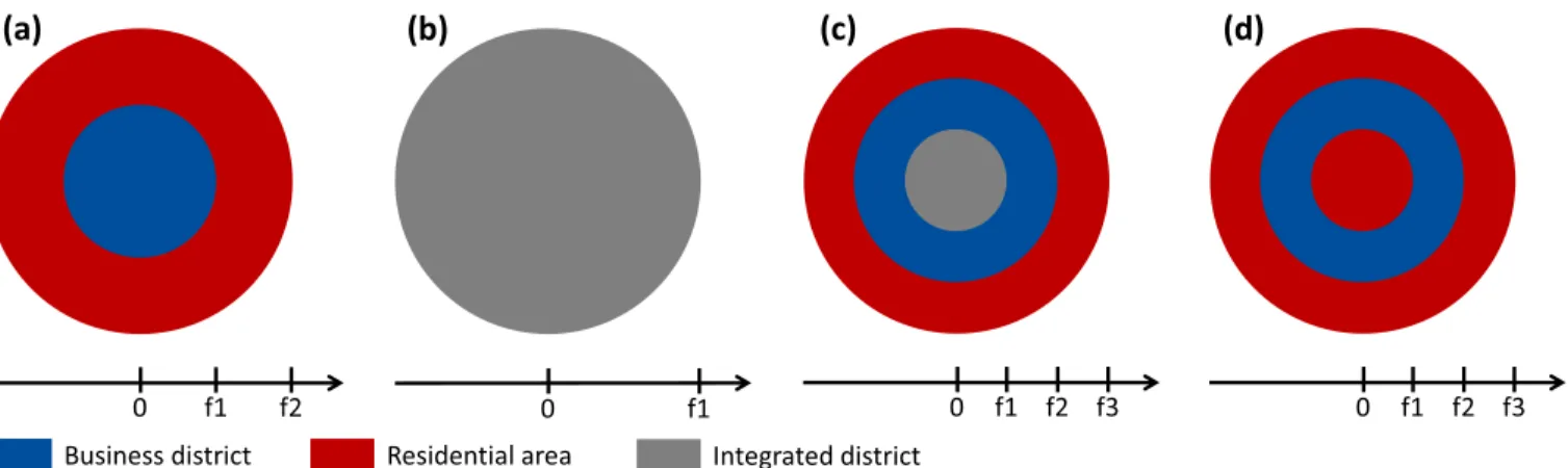
the four typical configurations we are interested in are the monocentric configuration, the completely mixed configuration, the incompletely mixed configuration (Fig 2a–2c), which
Fig 1. Diagram of the system dynamic.Reading starts by the outer-left box, withsrepresenting any state of the model, and follows the black arrows.
Hexagonal boxes indicate conditional statements and elliptic boxes stand for adaptation processes. doi:10.1371/journal.pone.0135871.g001
Fig 2. The four typical circular configurations of the static equilibrium model.The monocentric configuration(a), the completely mixed configuration
(b), the incompletely mixed configuration(c)and the rotational duocentric configuration(d)are different combinations of areas where only business firms locate (business districts), where only households locate (residential areas) or where both business firms and households colocate (integrated district). The fi
sdenote the distances from the respective boundaries to the city centre.
have been taken from Ogawa and Fujita [21], and the duocentric rotational configuration (Fig 2d), which is introduced here as a circular interpretation of the duocentric city from Fujita and Ogawa [20]. These configurations also prevent us from referring to unrealistic equilibria such as a circular city with a business district at its edge [22].
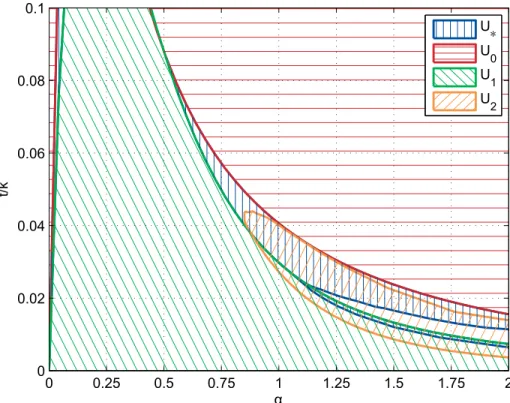
Equilibrium condition areas of the typical configurations have been truncated to relative commuting costs lower than 0.1 since this condition is necessary for a single production activ-ity to be profitable. That is required by the dynamic assumptions and thus makes other values irrelevant for further comparison with the simulated results. As one may have expected, the equilibrium conditions in a {α,t/k}-space are qualitatively similar to one-dimensional results
of Fujita and Ogawa [20] (Fig 3). More precisely, the duocentric equilibrium area overlaps other equilibrium areas such that in some parts of the figure, multiple equilibria are defined. Although the classic approach in urban static economics is to assume that exogenous historical events differentiate these equilibria [42], the dynamic assumptions of the following agent-based model will select a particular equilibrium. Yet there is also an area where the duocentric pattern is the only equilibrium. This is because of the split of the incompletely mixed equilib-rium area forα1.1. This is due to the constraint of no commuting in the integrated district,
see Fujita and Ogawa [20] (section 3.2.3, p.176) for further details. Among the differences with the one-dimensional equilibrium areas, note the curves’dilation along both thex-axis and the
y-axis, simply resulting from the ability of agents to agglomerate more compactly in a two-dimensional space.
Simulated configurations
Because our dynamic assumptions require a single production activity to be profitable, the rela-tive commuting cost must be lower than 0.1. Otherwise, business activities can not be created, even though population is growing, which lead to the trivial result of a forever empty region. Simulations have thus been performed on the subspaceα×t/k= [0, 2] × [0, 0.098], which
has been divided in 135 points. More precisely,kwas set to 100 whilsttandαwere varying
between runs.
Note that only one run of each parametrization has been realised. This low number results from a trade-off between the number of parametrizations and the number of runs for each of them. Due to the long running time of the model and lack of computer power, any number of runs large enough to proceed with valid statistical tests would have reduced the number of parametrizations to an insignificant value. Since this experiment is an heuristic one, the num-ber of parametrizations was thus given priority. Uncertainty issues are discussed further.
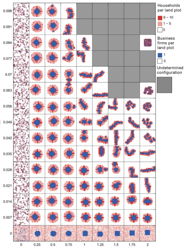
First, let’s have a look at extreme parameters results. For (α,t/k) = (0, 0), the simulated
long-term equilibrium is a fully random configuration since neither business firms nor households have any incentive to agglomerate nor to disperse (Fig 4). Along thet/k-axis, households locate nearby their hiring business and business firms locate randomly, thus leading to a dispersed configuration. Finally along theα-axis, business firms cluster and households locate randomly,
thus leading to a semi-dispersed configuration. These results show the consistence of our model with basic economic literature.
Forα6¼0 andt/k6¼0, long-term configurations present several kind of geometries which
will now be discussed regarding to their multicentricity and their circularity. However, for high values of bothαandt/k, no long-term configuration was reached (Fig 4). These
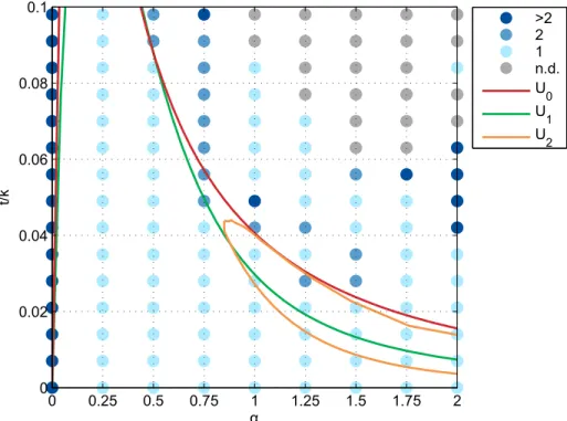
The multicentricity of simulated configurations was measured by the number of distinct business districts, which are themselves defined by 8-cells neighbourhood connectivity among business district plots. It appears that all long-term configurations under monocentric equilib-rium conditions are indeed monocentric ones (Fig 5). Under the equilibrium conditions of the other reference configurations however, the long-term configurations are not always mono-centric. Especially when bothαandt/kare high enough so that a completely integrated city
could be an equilibrium, the dynamic model leads to long-term configurations with 2, 3, up to 6 distinct business districts. Duocentric equilibrium configurations thus emerged in an area of the parameters space that is wider than the expected one. Yet for the (2, 0.084)-run, the full set-tling configuration is monocentric and qualitatively looks like a square-shaped incompletely mixed configuration.
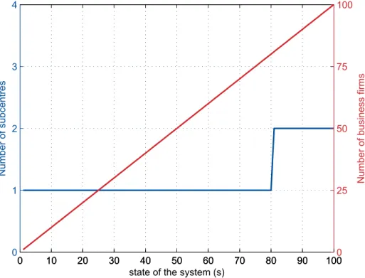
Regarding the dynamic preceding these multicentric configurations, it appears that two pro-cesses occurred. On the one hand, the region may develop following the growth of a single city centre until the next incoming business decide to settle a few land plots away from the existing business district, thus creating by itself a second centre which is in turn the starting point of a new urbanization process (Fig 6and firstgiffile inS1 File).
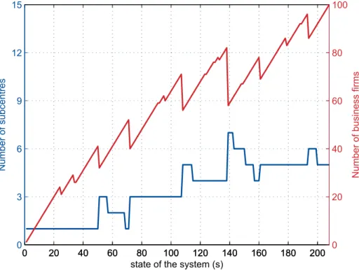
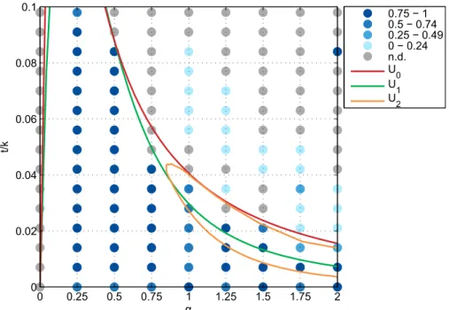
On the other hand, the region may develop following the growth of a single city centre until the next business settling on its border produces a wage rise that forces nearby firms to leave the agglomeration. Some other firms may in turn leave the city so that they break the initial city center in several subcentres. In this case, sudden growths in the number of city subcentres occur along with sudden falls in the number of business firms (Fig 7and secondgiffile inS1 Fig 3. Equilibrium conditions of the four typical circular configurations.Equilibrium conditions of the continuous incompletely mixed (U*), completely mixed (U0), monocentric (U1), and rotational duocentric (U2) urban configurations in the {α,t/k}-space whereαis the distance-decay parameter of the agglomeration economies andt/kis the relative commuting cost.
Fig 4. Simulated long-run equilibrium configurations.Long-run simulated configurations are given for 135 parametrizations onαandt/k, whereαis the distance-decay parameter of the agglomeration economies andt/kis the relative commuting cost. If no long-run equilibrium was reached, the configuration is set undetermined.
File). Afterwards, the following incoming business firms may thus either re-establish a physical link between the subcentres, or simply develop them separately.
Both paths to multicentricity can be regarded as two parts of the process described by Krug-man [27]. The former is the positive part of edge cities’creation, emphasizing the settling of businesses in attractive places, whilst the later emphasizes the negative part of the process, which is the leaving of businesses in unattractive land plots. These processes are distinguished here because of the different agents’displacement rate.
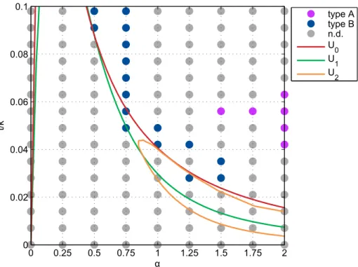
Looking at initial parameter values, it appears that runs where subcentres were created by incoming business firms had parameter values that are close to the limit equilibrium conditions of the completely mixed configuration (Fig 8). Conversely, those where subcentres were created by leaving business firms had parameter values under the completely mixed equilibrium condi-tions, forα>1.5 and 0.042t/k0.063.
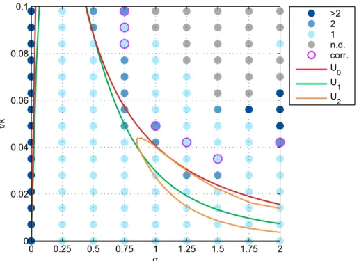
As previously mentioned, border effects occurred during the simulations because of the unexpected length of several configurations. For 7 runs, the city hit regionXboundary before getting its final number of subcentres. However, taking into account the number of subentres in the city before it reached the border does not change the results (Fig 9).
Regarding the monocentric configurations, the circularity index was measured as (1-E) whereEis the eccentricity of the ellipse that has the same second-moments as the city contour. The procedure, implemented in MatLab by theregionpropsfunction, consists in comput-ing the covariance matrix of the coordinates of pathes with at least one agent locatcomput-ing on them. Eigenvalues then give the lengths of the major and minor axis of the associate ellipse, from which the focal distance can be computed. The eccentricity of the associate ellipse, which is the ratio of its focal distance and its major axis length, can thus be computed.
Fig 5. Multicentricity of the simulated long-run equilibrium configurations.Blue color scale denotes the number of disconnected business districts in the simulated long-run equilibrium configurations for 135 parametrizations onαandt/k, whereαis the distance-decay parameter of the agglomeration economies and
Once more, it appears that all the long-term configurations under monocentric equilibrium conditions are well-circular ones, with a circularity index larger than 0.5 (Fig 10). Under the equilibrium conditions of the other reference configurations however, the long-term configura-tions that were monocentric were not circular at all. Instead, they grew marginally to an elon-gated long-term configuration with a circularity index that is lower than 0.24 for 19 runs out of 27 (see thirdgiffile inS1 File). Yet for the (2, 0.084)-run, the full settling configuration is a perfect square and thus presents a circularity of 1.
Discussion
Deducing practical knowledge from the previous experiment requires a good understanding of the involved parameters. Firstly, recallt/k, here named the relative commuting cost, is the ratio of the unitary commuting cost over the monetary conversation rate of the locational potential. Hence, all things otherwise being equal, highert/kratio means that commuting costs are high compared to the monetary benefit of the agglomeration economies. Secondly,αdescribes the
distance decay effect of the agglomeration economies. Hence,ceteris paribus, higherαvalue
means that agglomeration economies between two business firms are decreasing faster with distance.
In our agent-based simulation model, it appears that under parameter values for which the monocentric configuration stands as an equilibrium, the intermediate configurations never diverge a lot from this equilibrium. It means that for a given relative commuting cost, if agglom-eration economies extend far in space, then intermediate configurations always count a single business district and present a circular full settling configuration. This suggests that cities
Fig 6. Creation of subcentres by incoming firms during the (0.75, 0.056)-run.The curves depict the dynamics of the number of firms in the urban agglomeration and of the number of separated business districts during the simulation forα= 0.75 andt/k= 0.056, whereαis the distance-decay parameter of the
agglomeration economies andt/kis the relative commuting cost. The plot extends from the first state of the system (s= 1) to the long-run equilibrium (s= 100 here).
experiencing or implementing strong agglomeration forces undergo less variability in their con-figurations due to asynchronous development.
Under parameter values for which the other configurations stand as equilibria, which are for higher relative transport cost and distance-decay of the agglomeration economies than the monocentric equilibrium conditions, the configuration is far less stable. Under these condi-tions, for a given relative commuting cost, agglomeration economies decrease rapidly with dis-tance. Consequently, urban configurations grow marginally and tend to produce elongated configurations with time. Note that since the marginal growth process relies on strong centrip-etal forces, it can occur either through high relative commuting cost, through high distance-decay of the agglomeration economies or through any equivalent combination of both, which explains their range of occurrence (Fig 4) In this context also, multicentric configurations emerge in two ways.
Firstly, if the distance-decay of agglomeration economies is not too high, which means for a given relative cost that it is just higher than the monocentric conditions would require, subcen-tres may be created by the arrival of new business firms a few distance away from the previous city centre. This is because agglomeration economies extend far enough for them to benefit from the proximity of the previous city centre, whilst transport costs are too high for them to support wage levels at the boundary of the city centre.
Secondly, if the distance-decay of agglomeration economies is much higher than the mono-centric conditions would require, then elongated configurations may break apart in several subcentres. This is because the distance-decay of agglomeration economies is so high that busi-ness firms need a great proximity of other firms in order to stay productive. Meanwhile,
Fig 7. Creation of subcentres by moving firms during the (2, 0.049)-run.The curves depict the dynamics of the number of firms in the urban agglomeration and of the number of separated business districts during the simulation forα= 2 andt/k= 0.049, whereαis the distance-decay parameter of the agglomeration economies andt/kis the relative commuting cost. The plot extends from the first state of the system (s= 1) to the long-run equilibrium (s= 208 here).
transport costs are so high that if workers of a firm are pushed further from their employer because of the arrival of a new business firm, the employer can not pay them any more. Thus it is forced to leave its place and relocate, hence changing locational potential in its neighbour-hood and forcing in turn other firms to relocate.
These two processes repeat for different values of relative commuting cost, with the fol-lowing exceptions. For high relative commuting costs, breaks in urban configurations occurred so frequently under high distance-decay of agglomeration economies that a long-run equilibrium configuration could not have been reached by simulations. They often pres-ent a cyclic dynamics prevpres-enting all the population to settle, although long-term equilibrium may still occur as exemplified by the (2, 0.084)-run. In this context, the city seems not stabi-lizing easily by itself and urban planners should therefore either influence commuting costs and agglomeration economies, or coordinate agents location decisions in order to reach a sta-ble urban configuration.
In order to say more about the cyclic and chaotic dynamics of the model, an interesting experiment would be to run simulations with different ratio of development rates for busi-nesses and households. Indeed, this acts as a transmission delay in the feedbacks conducting agents’location decisions, which is well known to influence the model dynamic as in the classic prey-predator model [43,44].
As a cost of its simplicity, this exploratory model presents many technical or conceptual limitations that may be overcome. Although uneven mobility among agents was introduced in the dynamic setting, a more realistic assumption would be to fully distinguish agents from buildings. This would provide a two-dimensional examination of other economic studies (see for example Fujita [25] and Anas [45]).
Fig 8. Classification of multicentric configurations according to their apparition process. Type A
designates configurations where subcentres were created by leaving business firms whilsttype Bpoints out full settling configurations where subcentres were created by incoming business firms. Coloured lines delineate the equilibrium conditions of the continuous completely mixed (U0), monocentric (U1), and rotational duocentric (U2) urban configurations.
Although a single run for each parametrization was enough to show how intermediate con-figurations can differ from expected equilibria, several runs would be necessary to discuss the representativeness of simulated long-term configurations. However, initial conditions are invariable and randomness occurs only when similar land plots have the same value regard to the incoming agent, in which case the winning plot is chosen with even probability. Resulting configurations are thus expected to slightly change in orientation.
Finally, by taking an analytical equilibrium model as benchmark, this paper does not argue that the study equilibrium conditions of dynamic systems, including for example the conver-gence conditions, is useless. Actually suchex-anteanalysis would help to discuss the cyclic dynamics occurring under high-valued parameters. We simply mean here that agent-based simulation models can easily be designed more consistently with economic literature by this way.
Conclusion
As a conclusion, our model of urban morphogenesis of a two-sector city with heterogeneous mobility under exogenous population growth shows that urban development is stable and ends up with more homogeneous long-term configurations under strong agglomeration effects. For low agglomeration effects however, urban development is more changing, configurations vary-ing a lot in the number of subcentres and in circularity. More precisely, we have pointed out two different dynamic processes of multicentricity, involving leaving business firms or not, that are well distinguished in terms of commuting cost and agglomeration economies’extents. We have also highlighted a dynamic marginal urbanization leading to elongated long-run
Fig 9. Pre-border corrected multicentricity of the simulated long-run equilibrium configurations.Blue color scale denotes the number of disconnected business districts in the simulated long-run equilibrium configurations for 135 parametrizations onαandt/k, whereαis the distance-decay parameter of the agglomeration economies andt/kis the relative commuting cost. Pink circles highlight the runs that underwent border effects. Coloured lines delineate the equilibrium conditions of the continuous completely mixed (U0), monocentric (U1), and rotational duocentric (U2) urban configurations.
configurations. Finally, for extremely low agglomeration forces, repeated moves of agents strive against the stabilization of the urban configuration.
Consequently, little variations in parameters and path-dependency effects may conduct cit-ies to very different configurations in the long run. All things otherwise being equal, higher rel-ative commuting cost and distance-decay of agglomeration economies produce more changing urban configurations that require an exogenous intervention to be stabilized. Consequently, this paper warns urban planning policy makers against the difference that may stand between appropriate long-term perspectives, represented here by analytic equilibrium configurations, and short-term urban configurations, simulated here following basic dynamic assumptions.
Supporting Information
S1 File. Supporting information archive.Contains anlogofile, which is the model implemen-tation in Netlogo, and threegiffiles, which show the dynamics of agents’location in regionX
during the simulations with (α,t/k) equals to (0.75, 0.056), (2.00, 0.049) and (1.75, 0.042).
(ZIP)
Acknowledgments
We would like to thank Joe Tharakan and Geoffrey Caruso for their insightful comments.
Author Contributions
Conceived and designed the experiments: JD DP IT. Performed the experiments: JD DP IT. Analyzed the data: JD DP IT. Contributed reagents/materials/analysis tools: JD DP IT. Wrote the paper: JD DP IT.
Fig 10. Circularity of the simulated long-run equilibrium configurations.Blue color scale denotes the number of disconnected business districts in the simulated long-run equilibrium configurations for 135 parametrizations onαandt/k, whereαis the distance-decay parameter of the agglomeration economies and
t/kis the relative commuting cost. Coloured lines delineate the equilibrium conditions of the continuous
References
1. World Bank. Urban population (% of total). In: World Bank Open Data. Washington D. C., United States: The World Bank Group; 2015. Available from:http://data.worldbank.org/ indicator/SP.URB.TOTL.IN.ZS/countries?display = graph.
2. United Nations, Department of Economic and Social Affairs, Population Division. Annual Percentage of Population at Mid-Year Residing in Urban Areas. World data for years 2005–2009 acquired via website. In: World Urbanization Prospects: The 2014 Revision. New-York, United-States: United Nations; 2014. Available from:http://esa.un.org/unpd/wup/DataQuery/.
3. World Bank. Population in urban agglomerations of more than 1 million (% of total population). In: World Bank Open Data. Washington D. C., United States: The World Bank Group; 2015. Available from: http://data.worldbank.org/indicator/EN.URB.MCTY.TL.ZS/countries?display = graph.
4. A planet of suburbs. The Economist. 2014 Dec;p. 43–48. Available from:http://www.economist. com/suburbs.
5. Bai X, Shi P, Liu Y. Society: Realizing China’s urban dream. Nature News. 2014 May; 509(7499):158. Available from: http://www.nature.com/news/society-realizing-china-s-urban-dream-1.15151. doi:10.1038/509158a
6. Curtin E. New garden city must avoid a‘slash-and-burn’approach to national housing issue. The Con-versation. 2014 Dec;Available from: https://theconversation.com/new-garden-city-must-avoid-a-slash-and-burn-approach-to-national-housing-issue-35053.
7. 1,5 milliard pour créer La Louvière-la-Neuve. La Libre Belgique, édition du 19/02/2014.
8. Starting from scratch. The Economist. 2013 Sep;Available from:http://www.economist.com/ news/briefing/21585003-building-city-future-costly-and-hard-starting-scratch.
9. Barthelemy M, Bordin P, Berestycki H, Gribaudi M. Self-organization versus top-down planning in the evolution of a city. Sci Rep. 2013 Jul;3.
10. Glaeser EL, Kahn ME. The greenness of cities: Carbon dioxide emissions and urban development. Journal of Urban Economics. 2010; 67(3):404–418. doi:10.1016/j.jue.2009.11.006
11. Glaeser E. Triumph of the City: How Our Greatest Invention Makes Us Richer, Smarter, Greener, Healthier, and Happier. New-York, United-States: Penguin Group, Penguin Press; 2011.
12. Wenban-Smith HB. The influence of urban form on spatial costs. Recherches Economiques de Lou-vain. 2011; 77(2–3):23–46. doi:10.3917/rel.772.0023
13. Howard E. Garden Cities of Tomorrow. London, United-Kingdom: Swan Sonnenschein & Company; 1902.
14. Fujita M, Thisse JF. Economics of Agglomeration. Cities, Industrial Location and Globalization. 2nd ed. Cambridge, United-Kingdom: Cambridge University Press; 2013.
15. von Thünen JH. Der Isolierte Staat in Beziehung auf Landwirtschaft und Nationalökonomie (L’Etat Isolé dans ses relations avec l’agriculture et l’économie nationale). In: von Thünen—Economie et espace. (1994) ed. Paris, France: Economica; 1842. p. 352.
16. Alonso W. Location and land use. Cambridge, United-States: Harvard University Press; 1964.
17. Muth RF. Cities and housing: the spatial pattern of urban residential land use. Chicago, United States: University of Chicago press; 1969.
18. Mills E. Studies in the Structure of the Urban Economy. Baltimore, United-States: The Johns Hopkins Press; 1972.
19. Brueckner JK. The structure of urban equilibria: A unified treatment of the muth-mills model. In: Hand-book of Regional and Urban Economics. vol. 2; 1987.
20. Fujita M, Ogawa H. Multiple Equilibria and Structural Transition of Non-Monocentric Urban Configura-tions. Regional Science and Urban Economics. 1982; 12(2):161–196. doi:10.1016/0166-0462(82) 90031-X
21. Ogawa H, Fujita M. Nonmonocentric Urban Configurations in a Two-Dimensional Space. Environment and Planning A. 1989; 21(3):363–374. doi:10.1068/a210363
22. Lucas RE, Rossi-Hansberg E. On the Internal Structure of Cities. Econometrica. 2002; 70(4):1445– 1476. doi:10.1111/1468-0262.00338
23. Carlier G, Ekeland I. Equilibrium structure of a bidimensional asymmetric city. Nonlinear Analysis: Real World Applications. 2007; 8(3):725–748. doi:10.1016/j.nonrwa.2006.02.008
25. Miyao T. Dynamic urban models. In: Mills ES, editor. Handbook of Regional and Urban Economics. vol. 2. Amsterdam, The Netherlands: Elsevier; 1987. p. 877–925.
26. Krugman P. On the number and location of cities. European Economic Review. 1993 Apr; 37(2– 3):293–298. doi:10.1016/0014-2921(93)90017-5
27. Krugman P. The self-organizing economy. Cambridge (Mass.): Blackwell; 1996.
28. Garreau J. Edge City: Life on the New Frontier. Anchor Books; 1991.
29. Manson SM, Sun S, Bonsal D. Agent-Based Modeling and Complexity. In: Heppenstall AJ, Crooks AT, See LM, Batty M, editors. Agent-Based Models of Geographical Systems. London, United-Kingdom: Springer; 2012. p. 125–139.
30. Tesfatsion L. Agent-based computational economics: modeling economies as complex adaptive sys-tems. Information Sciences. 2003; 149(4):262–268. doi:10.1016/S0020-0255(02)00280-3
31. Tesfatsion L, Judd KL, editors. Handbook of computational economics. Agent-based computational economics. vol. 2. Amsterdam, The Netherlands: Elsevier; 2006.
32. Fujita M, Mori T. Frontiers of the New Economic Geography. Papers in Regional Science. 2005; 84 (3):377–405. doi:10.1111/j.1435-5957.2005.00021.x
33. Heikkila EJ, Wang Y. Fujita and Ogawa revisited: an agent-based modeling approach. Environment and Planning B: Planning and Design. 2009; 36(4):741–756. doi:10.1068/b34080
34. Yang JH, Ettema D. Modelling the Emergence of Spatial Patterns of Economic Activity. Journal of Artifi-cial Societies and SoArtifi-cial Simulation. 2012; 15(4):6.
35. Li Q, Yang T, Zhao E, Xia X, Han Z. The Impacts of Information-Sharing Mechanisms on Spatial Market Formation Based on Agent-Based Modeling. PLoS ONE. 2013; 8(3):e58270. doi:10.1371/journal. pone.0058270PMID:23484007
36. Delloye J. Two-dimensional non-circular urban configurations. An integrated analytic and agent-based approach. Mémoire de fin d’études en sciences géographiques. Louvain-la-Neuve, Belgium: Univer-sité Catholique de Louvain; 2014.
37. Wilensky U. NetLogo [software]. Evanston, United-States: Northwestern University, Center for Con-nected Learning and Computer-based Modeling; 1999.
38. MathWorks. MatLab 7.10.0.499 (R2010a) [software]. Natick, United-States: The MathWorks Inc.; 2010.
39. Wegener M, Gnad F, Vannahme M. The time scale of urban change. In: Hutchinson B, Batty M, editors. Advances in urban systems modelling. Amsterdam, The Netherlands: Elsevier; 1986. p. 175–197.
40. Simmonds D, Waddell P, Wegener M. Equilibrium versus dynamics in urban modelling. Environment and Planning B: Planning and Design. 2013; 40(6):1051–1070. doi:10.1068/b38208
41. Glaeser EL. Cities, Agglomeration, and Spatial Equilibrium. The Lindahl Lectures. Oxford, United-King-dom: Oxford University Press; 2008.
42. Fujita M, Krugman P, Venables AJ. The spatial economy: Cities, regions, and international trade. Cam-bridge and London:; 1999.
43. Lotka AJ. Elements of Physical Biology. Williams & Wilkins Company; 1925.
44. Volterra V. Variazioni e fluttuazioni del numero d’individui in specie animali conviventi. Memorie della Accademia dei Lincei. 1926; 2:31–113.