N ATIONALS YSTEM OF

(1)

N

ATIONAL

S

YSTEM OF

I

NNOVATION AND

T

ECHNOLOGICAL

D

IFFERENTIATION

:

A

M

ULTI

-

COUNTRY

E

VOLUTIONARY

M

ODEL

(Preliminary Version)

Américo T. Bernardes, Universidade Federal de Ouro Preto – Departamento de Física

Ricardo M. Ruiz, Universidade Federal de Minas Gerais – CEDEPLAR*

Leonardo C. Ribeiro, Universidade Federal de Minas Gerais – Departamento de Física

Eduardo M. Albuquerque, Universidade Federal de Minas Gerais – CEDEPLAR

* Address:

Rua Curitiba 832 / 7th floor

30170-120, Belo Horizonte, Minas Gerais, Brazil. E-mail: [email protected].

Abstract:

The paper introduces an agent-based model in which the national system of innovation (NSI) is a main determinant of the wealth of nations. The model is defined as a self-organizing economy where agents are countries with their own capabilities for imitation and innovation. The interactions among countries are given by the relative competitiveness of a country in world economy, which is represented by functions that connect their prices, demands, technologies, and incomes. The simulations show that the model reproduces countries hierarchies that have been found in several empirical studies.

Key words: national system of innovation, technological change, innovation, growth

JEL: O33, 041, F43, C68

(2)

1. INTRODUCTION

Recently, by using statistics of patents (USPTO) and scientific papers (ISI), we have studied the interplay between science and technology and its influences on the level of development (country GNP per capita). We have identified strong relations among these three variables and threshold levels in the scientific production, beyond which the use of scientific output by the technological sector increases (Bernardes & Albuquerque, 2003).

In this work, we present a simple model that aims to reproduce those correlations and the hierarchy of countries of our empirical studies. We created an artificial world economy populated by agents (countries) where the interactions among countries are represented by functions that connect their prices, demands, technologies, and incomes.1

Starting from random values for the country technology and income, the artificial world economy self-organizes itself and creates hierarchies of countries that are similar to the ones found in our empirical studies. Technology is measured, and we show that it is proportional to the country’s production of patents and scientific articles, which are conventional proxies of the national systems of innovation efficiency.

2. COUNTRY ECONOMIC STRUCTURE (INTERNAL RULES)

2.1.PRICE AND PRODUCTION

The equations that define the level of production and price are:

Qi = (Ti . Li) + Vi (1)

Pi = (Yi / Qi) (2)

Pi = Yi / [(Ti . Li) + Vi]

Where Qi is the amount of goods produced by country i, Ti represents country technology, Li

stands for population or labor force, and Vi is the unsold good of previous period. The country

income (US$ GDP) is Yi and Pi is the price of one unit of good Qi. Population (or labor force)

is constant; thus Qi depends mostly on Ti, which is the output of the national system of

innovation. The price level is set by an adaptive rule: everything else constant, unsold stock and decreasing national income reduce prices and increase competitiveness, while falling inventory and raising income do the opposite.

2.2.COMPETITIVENESS

The country competitiveness Ci has an inverse relation with its price:

Ci = (1 / Pi) (3)

1

(3)

The global competitiveness Cg is defined by the country competitiveness Ci weighted by its

market share Mi (the share of the country in the world economy measured by its income):

Mi = Yi / ∑Yi

Cg = ∑(Mi . Ci) (4)

2.3.TECHNOLOGICAL CHANGE

Countries change their technology in order to increases its competitiveness and wealth. To do so, it must change its technology, which depends on the previous level of its own knowledge (Ti), on the technological information spilled from international sources (Tg). Country

capabilities to create new technologies are represented by patents and articles per capita (PATi

and ARTi):

Ti2 = Ti1 + Ni (5)

Ni = (Tg . PTi . ATi)1/3, where 0 < Ni (6)

Tg = ∑(Mi . Ti) (7)

The coefficient Ni is a proxy to the national system of innovation, which corresponds to the

countries innovation capabilities plus the spillovers of technologies of the global economy (Tg). Therefore, the national system of innovation Ni summarizes the country capabilities to imitate and innovate when other countries increase their competitiveness by technological changes.

2.4.INCOME

The country income is Yi plus the income not spent in the previous period Si (savings). The wage or per capita income is the country income distributed among its population.

Yi = Ki + Si (8)

Wi = Yi / Li (9)

The global income is the sum of all country incomes:

Yg = ∑Yi (10)

3.COUNTRY DEMAND,CAPITAL AND SAVINGS

3.1.MARKET SHARE AND DEMAND

(4)

the σ is the speed of the market share changes due to asymmetries in the country and the global competitiveness.

Mi2 = Mi1 . [1 + σ . {(Ci / Cg) – 1}], where 0 < σ < 1, and ∑Mi = 1 (11)

The country´s demand DYi (units of money) is a share Mi of the global income:

DYi = Mi . Yg

The country´s demand Di (unit of goods) is given by:

Di = Dyi / Pi = (Mi . Yg) / Pi (12)

3.2.CAPITAL,INVENTORY AND SAVINGS

There is recurrent disequilibrium on the amount of goods demanded and supplied. Thus, three simple rules were created:

When Di = Qi, then: Ki = Pi . Qi (13)

Sg = Sg + Si = Sg + 0 Vg = Vg + Vi = Vg + 0

When Di > Qi, then: Ki = Pi . Qi (14)

Sg = Sg + Si = Sg + [Pi . (Di - Qi)] Vg = Vg + Vi = Vg + 0

When Di < Qi, then: Ki = Pi . Di (15)

Sg = Sg + Si = Sg + 0

Vg = Vg + Vi = Vg + (Qi – Di)

Where Ki is the capital or sales, Si and Sg are the country and global saving (not spent income), and Vi and Vg are the country and global stock of unsold goods. The country savings is proportional to its market share Mi:

Si = Sg . Mi (16)

(5)

(equations 14), there is an excess of demand (Sg > 0), there is no inventory (Vi = 0) and consumers do not spend all their income, which means savings Si is added to the global saving and then distributed to countries (equation 16). In the third case (equation 15) there is an excess of supply, stock is positive (Vi > 0) and all income is spent (Sg = 0).

At steady state, there is no inventory (Vg = ΣVi = 0), which is a first measure of equilibrium in the artificial world economic system. When all countries spend their income, there is no saving (Sg = ΣSi = 0), which means the demand side is also at steady state. Global savings Sg is a second measure of equilibrium.

4.ABASIC ECONOMETRIC ANALYSIS

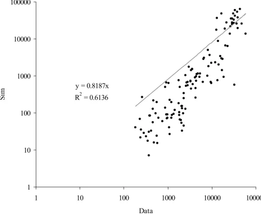
Table 1 to 4 shows some econometric relationships and models. The GNP is the dependent variable, and patents, articles, and population are the independent variables; all in logarithmic scale. As one can see there are strong relationships among all variables, which means that some “system” (set of iteration / interaction) connects them. Three basic econometric models show these relationships:

Model 1: GNP = α + β1.POP + β2.PATpc + β3.ARTpc

Model 2: GNP = α + β1.POP + β2.PAT + β3.ART

Model 3: GNPpc = α + β1.POP + β2.PATpc + β3.ARTpc

Models 1 and 3 are those with the same basic setup of the model of proposed above. Model 2 is the one with the best fit, although it presents some econometric problem, such as multicollinarity (see table 1 for correlations).

The agent-based model uses the same variable of the econometric model as a determinant of the GNP and GNPpc. Nonetheless, there is an “imitation behavior” represented by the term Tg in the equation 6 that is not a component of the econometric model. The usual proxies for technological capabilities PAT and ART do not capture the imitation capability, and there is no good proxy for such behavior. Thus, the agent-based model introduced the imitation into the determinants of the wealth of nations, and the simulation shows that its relevance.

5.ILLUSTRATIVE SIMULATIONS AND DISCUSSION

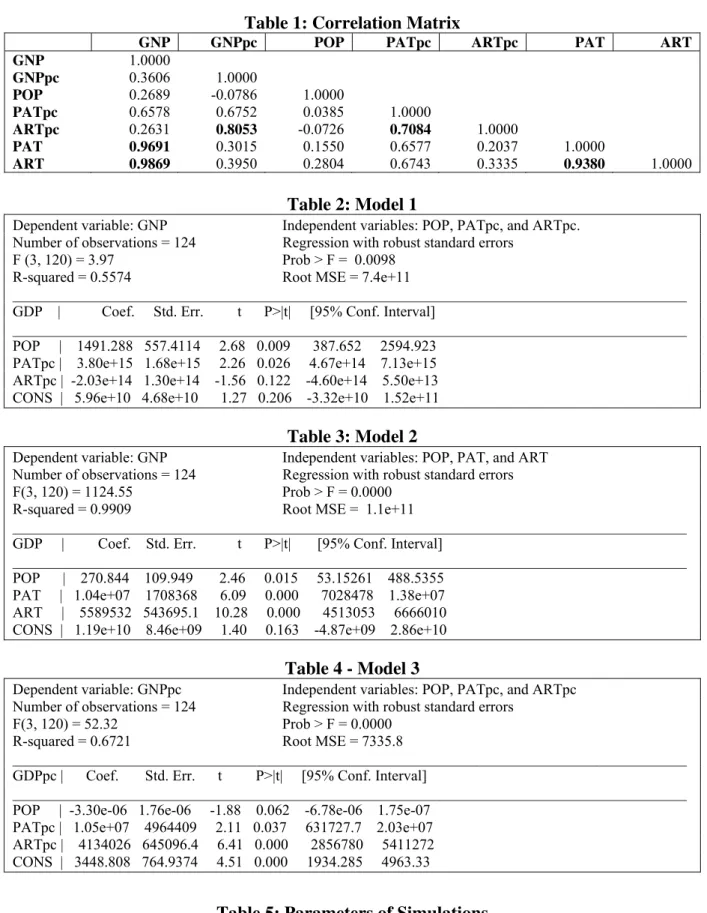
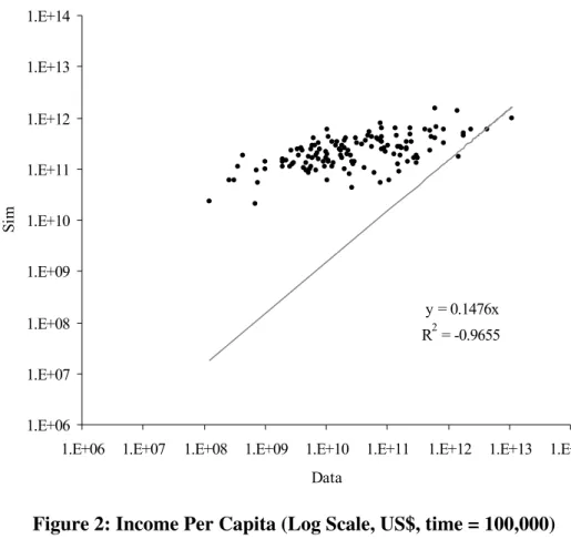
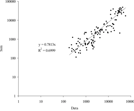
The figures below summarize the simulations. Figures 1 and 2 show the fitness of the model when all independent variables are random numbers in the interval [0, 1], except for the population, which is the one of the period 1999-2003. Figures 3 and 4 show the same correlations when the initial technology and income share are random numbers in the interval [0, 1], excluding the population and the NSI, which is given by the equation 6.

(6)

the model. Hence, we can say that imitation and the technological spillovers in an important determinant in technological race and the wealth of nations.

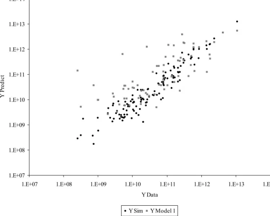
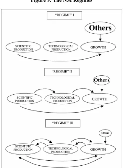
Figure 3 has another important characteristic: the slope of the fit line is 1.0976, which means that the larger and hi-tech economies are overestimated and the smaller economies are underestimated. A possible theoretical explanation for this result is that the model does not take into account the “other factors”, as described by Bernardes & Albuquerque (2003). Bernardes & Albuquerque (2003) suggest three different “regimes”, ranging from the least developed countries (regime I) to the developed countries (regime III) (figure 9). The model uses four sets of variables: scientific production, technological production, economic growth, and “others” (representing a broad range of factors and variables left out, such as availability of natural resources, health conditions, demographic factors etc.). The mutual feedback between scientific and technological capabilities and growth contribute to explain the share of the countries in the world economy (Fagerberg, 1994; Dosi et al., 1994).

As the country evolves, more connections are “turned on” and more interactions operate (the arrows in figure 7). “Regime III” is the case where all connections and interactions are working. As long as the development takes place, the role of “others” in the causation of economic growth decreases. In other words, as a country upgrades its economic position, its economic growth is more and more a result of its scientific and technological resources. The model proposed above has no proxy for “other factors”; thus those countries with GNP relying on “other factors” would have their share in the world economy underestimated, which is represented by a fit line with slope higher than 1. The difference between 1 and 1.0976 is a broad measure of “other factors”.

(7)

Table 1: Correlation Matrix

GNP GNPpc POP PATpc ARTpc PAT ART

GNP 1.0000

GNPpc 0.3606 1.0000

POP 0.2689 -0.0786 1.0000

PATpc 0.6578 0.6752 0.0385 1.0000

ARTpc 0.2631 0.8053 -0.0726 0.7084 1.0000

PAT 0.9691 0.3015 0.1550 0.6577 0.2037 1.0000

ART 0.9869 0.3950 0.2804 0.6743 0.3335 0.9380 1.0000

Table 2: Model 1

Dependent variable: GNP Independent variables: POP, PATpc, and ARTpc. Number of observations = 124 Regression with robust standard errors

F (3, 120) = 3.97 Prob > F = 0.0098 R-squared = 0.5574 Root MSE = 7.4e+11

__________________________________________________________________________________________ GDP | Coef. Std. Err. t P>|t| [95% Conf. Interval]

__________________________________________________________________________________________ POP | 1491.288 557.4114 2.68 0.009 387.652 2594.923

PATpc | 3.80e+15 1.68e+15 2.26 0.026 4.67e+14 7.13e+15 ARTpc | -2.03e+14 1.30e+14 -1.56 0.122 -4.60e+14 5.50e+13 CONS | 5.96e+10 4.68e+10 1.27 0.206 -3.32e+10 1.52e+11

Table 3: Model 2

Dependent variable: GNP Independent variables: POP, PAT, and ART Number of observations = 124 Regression with robust standard errors F(3, 120) = 1124.55 Prob > F = 0.0000

R-squared = 0.9909 Root MSE = 1.1e+11

__________________________________________________________________________________________ GDP | Coef. Std. Err. t P>|t| [95% Conf. Interval]

__________________________________________________________________________________________ POP | 270.844 109.949 2.46 0.015 53.15261 488.5355

PAT | 1.04e+07 1708368 6.09 0.000 7028478 1.38e+07 ART | 5589532 543695.1 10.28 0.000 4513053 6666010 CONS | 1.19e+10 8.46e+09 1.40 0.163 -4.87e+09 2.86e+10

Table 4 - Model 3

Dependent variable: GNPpc Independent variables: POP, PATpc, and ARTpc Number of observations = 124 Regression with robust standard errors

F(3, 120) = 52.32 Prob > F = 0.0000 R-squared = 0.6721 Root MSE = 7335.8

__________________________________________________________________________________________ GDPpc | Coef. Std. Err. t P>|t| [95% Conf. Interval]

__________________________________________________________________________________________ POP | -3.30e-06 1.76e-06 -1.88 0.062 -6.78e-06 1.75e-07

PATpc | 1.05e+07 4964409 2.11 0.037 631727.7 2.03e+07 ARTpc | 4134026 645096.4 6.41 0.000 2856780 5411272 CONS | 3448.808 764.9374 4.51 0.000 1934.285 4963.33

Table 5: Parameters of Simulations 1 – Country per capita income (2003)

2 - Global income is constant (Yg = ∑Yi) (2003) 3 - Country population is constant (mean of 1999-2003)

4 - PTpci, standardized by PTMAX (accumulated of 1999 to 2003) 5 - ATpci, standardized by ATMAX (accumulated of 1999 to 2003) 6 - Mi0 is random number Є [0, 1], where ∑Mi0 = 1

(8)

Figure 1: Country GNP (Log Scale, US$, time = 100,000)

(Random values of Pati, Arti, Ti0, Mi0, and Yi0)

y = 0.1476x

R2 = -0.9655

1.E+06 1.E+07 1.E+08 1.E+09 1.E+10 1.E+11 1.E+12 1.E+13 1.E+14

Data

Si

m

Figure 2: Income Per Capita (Log Scale, US$, time = 100,000)

(Random values of Pati, Arti, Ti0, Mi0, and Yi0)

y = 2.5906x

R2 = -0.1268

1 10 100 1000 10000 100000

Data

Si

(9)

(Ni as given by equation 2 and random values of Ti0, Mi0, and Yi0)

y = 1.0976x

R2 = 0.9889

1.E+06 1.E+07 1.E+08 1.E+09 1.E+10 1.E+11 1.E+12 1.E+13 1.E+14

Data

Si

m

Figure 4: GNP Per Capita (Log Scale, US$, time = 100,000)

(Ni as given by equation 6 and random values of Ti0, Mi0, and Yi0)

y = 0.7813x

R2 = 0.6999

1 10 100 1000 10000 100000

Data

Si

(10)

(Ni without the term Tg, and random values of Ti0, Mi0, and Yi0)

y = 1.3293x

R2 = 0.9653

1.E+06 1.E+07 1.E+08 1.E+09 1.E+10 1.E+11 1.E+12 1.E+13 1.E+14

Data

Si

m

Figure 6: GNP Per Capita (Log Scale, US$, time = 100,000)

(Ni without the term Tg, and random values of Ti0, Mi0, and Yi0)

y = 0.8187x

R2 = 0.6136

1 10 100 1000 10000 100000

Data

Si

(11)

Figure 7: GDP Prediction - Simulation and Econometric Model 1 (ln scale)

1.E+07 1.E+08 1.E+09 1.E+10 1.E+11 1.E+12 1.E+13 1.E+14

1.E+07 1.E+08 1.E+09 1.E+10 1.E+11 1.E+12 1.E+13 1.E+14 Y Data

Y P

re

d

ic

t

Y Sim Y Model 1

Figure 8: GDP Prediction - Simulation and Econometric Model 2 (ln scale)

1.E+07 1.E+08 1.E+09 1.E+10 1.E+11 1.E+12 1.E+13 1.E+14

1.E+07 1.E+08 1.E+09 1.E+10 1.E+11 1.E+12 1.E+13 1.E+14 Y Data

Y P

re

d

ic

t

(12)

Figure 9: The NSI Regimes

(13)

Appendix 1: Country Data Country Population (2003) Income p.c. (2003) Patent (1999-2003) Articles (1999-2003)

1 Albania 3169064.0 1800.1997 1.0 159.0 2 Algeria 31832610.0 2136.7587 1.0 2322.0 3 Angola 13522110.0 1022.4025 0.0 52.0 4 Antigua and Barbuda 78580.0 9662.2423 1.0 5.0 5 Argentina 37869730.0 3422.1464 266.0 21941.0 6 Armenia 3055630.0 917.9135 5.0 1669.0 7 Australia 19881000.0 26275.2139 4046.0 97116.0 8 Austria 8090000.0 31288.7597 2695.0 35529.0 9 Azerbaijan 8233000.0 866.9391 3.0 851.0 10 Bahamas 317413.0 16571.4700 55.0 34.0 11 Bahrain 711662.0 13498.8787 2.0 305.0 12 Bangladesh 138066400.0 376.0050 1.0 1985.0 13 Barbados 270584.0 9707.9983 4.0 185.0 14 Belarus 9880963.0 1783.3879 22.0 5304.0 15 Belgium 10376000.0 29095.6218 3404.0 48840.0 16 Belize 273700.0 3739.0391 2.0 27.0 17 Benin 6720250.0 529.3141 0.0 308.0

18 Bhutan 873663.0 681.7320 0.0 17.0

19 Bolivia 8814158.0 917.7827 3.0 440.0 20 Bosnia and Herzegovina 3832000.0 1819.6234 2.0 165.0 21 Botswana 1722468.0 4371.7317 0.0 464.0 22 Brazil 176596300.0 2863.8568 525.0 56652.0 23 Brunei 356447.0 15064.6000 0.0 156.0 24 Bulgaria 7823000.0 2548.7602 18.0 7540.0 25 Burkina Faso 12109230.0 345.3452 0.0 424.0 26 Burundi 7205982.0 82.6397 0.0 38.0 27 Cambodia 13403640.0 308.3868 0.0 89.0 28 Cameroon 16087470.0 776.4350 0.0 1025.0 29 Canada 31630000.0 27079.4441 17108.0 151612.0 30 Cape Verde 469681.0 1697.5649 0.0 5.0 31 Central African Republic 3880847.0 309.9859 0.0 65.0

32 Chad 8581741.0 303.9210 0.0 45.0

33 Chile 15774000.0 4590.6080 61.0 10203.0 34 China 1288400000.0 1099.4976 990.0 169568.0 35 Hong Kong, China 6816000.0 22758.6379 1080.0 3669.0 36 Colombia 44584000.0 1793.4194 42.0 3120.0

37 Comoros 600142.0 531.4792 1.0 7.0

(14)

50 Ecuador 13007940.0 2091.1042 11.0 569.0 51 Egypt 67559040.0 1220.0756 28.0 12455.0 52 El Salvador 6533215.0 2286.8220 4.0 44.0 53 Equatorial Guinea 494000.0 5900.1194 0.0 13.0 54 Eritrea 4389500.0 170.9965 0.0 84.0 55 Estonia 1353000.0 6712.5432 13.0 2736.0 56 Ethiopia 68613470.0 96.9450 0.0 1128.0

57 Fiji 835000.0 2685.7353 4.0 160.0

58 Finland 5212000.0 31058.2987 3673.0 35639.0 59 France 59762000.0 29410.2083 19584.0 232646.0

60 Gabon 1344433.0 0.0000 0.0 280.0

61 Gambia 1420895.0 257.8938 1.0 291.0 62 Georgia 4568000.0 874.8341 9.0 1206.0 63 Germany 82541000.0 29114.7465 53555.0 318198.0 64 Ghana 20669260.0 368.8666 1.0 797.0 65 Greece 11033000.0 15608.0091 109.0 25807.0 66 Grenada 104600.0 4181.6444 0.0 13.0 67 Guatemala 12307090.0 2009.3995 6.0 207.0 68 Guinea 7908905.0 459.0302 1.0 409.0 69 Guinea-Bissau 1489209.0 160.2488 0.0 80.0

70 Guyana 768888.0 964.2861 0.0 56.0

71 Haiti 8439799.0 345.8862 1.0 45.0

72 Honduras 6968512.0 985.5786 5.0 109.0 73 Hungary 10128000.0 8173.4540 255.0 20384.0 74 Iceland 289000.0 36377.0450 74.0 1549.0 75 India 1064399000.0 564.2973 1010.0 89887.0 76 Indonesia 214674200.0 1111.1027 31.0 2165.0 77 Iran 66392020.0 2065.6659 3.0 8702.0 78 Ireland 3994000.0 38487.4477 659.0 18933.0 79 Israel 6688000.0 16481.2848 4729.0 44086.0 80 Italy 57646270.0 25471.0952 8388.0 158657.0 81 Jamaica 2642628.0 2843.4865 7.0 641.0 82 Japan 127573000.0 33712.9168 165999.0 361295.0 83 Jordan 5307895.0 1873.8391 6.0 2469.0 84 Kazakhstan 14878100.0 2072.4191 11.0 994.0 85 Kenya 31915850.0 450.4280 13.0 2607.0

86 Kiribati 96377.0 605.9537 0.0 0.0

(15)

99 Madagascar 16893900.0 324.0261 3.0 106.0 100 Malawi 10962010.0 155.1894 0.0 496.0 101 Malaysia 24774250.0 4187.2846 216.0 4699.0 102 Maldives 293080.0 2356.9708 0.0 10.0 103 Mali 11651500.0 373.0000 0.0 221.0 104 Malta 399000.0 11951.1679 8.0 214.0 105 Marshall Islands 57000.0 1839.5614 2.0 0.0 106 Mauritania 2847869.0 415.1933 0.0 73.0 107 Mauritius 1222188.0 4288.5849 1.0 200.0 108 Mexico 102291000.0 6247.6186 411.0 24749.0 109 Moldova 4237600.0 467.4429 2.0 857.0 110 Mongolia 2479568.0 513.9851 0.0 221.0 111 Morocco 30112640.0 1452.1015 5.0 5213.0 112 Mozambique 18791420.0 229.9227 0.0 166.0 113 Myanmar 49362500.0 0.0000 0.0 94.0 114 Namibia 2014546.0 2120.0077 1.0 200.0 115 Nepal 24659960.0 237.2600 1.0 583.0 116 Netherlands 16221800.0 31531.7694 6536.0 88059.0 117 New Zealand 4009200.0 19856.5686 620.0 19371.0 118 Nicaragua 5480000.0 754.5954 2.0 109.0 119 Niger 11762250.0 232.2190 6.0 215.0 120 Nigeria 136461000.0 422.2578 11.0 3638.0 121 Norway 4562000.0 48411.6171 1241.0 23100.0 122 Oman 2598832.0 8349.2546 0.0 1130.0 123 Pakistan 148438800.0 554.7737 8.0 3157.0

124 Palau 19700.0 6289.3401 0.0 14.0

(16)

148 Somalia 9625918.0 128.0300 0.0 3.0 149 South Africa 45828700.0 3609.8372 566.0 17173.0 150 Spain 41101430.0 20404.4578 1373.0 112349.0 151 Sri Lanka 19231760.0 948.7640 4.0 928.0 152 St. Lucia 160588.0 4319.7499 0.0 7.0 153 St. Vincent / the Grenadines 109164.0 3447.0705 0.0 2.0 154 Sudan 33545730.0 530.3681 0.0 452.0 155 Suriname 438104.0 2329.4400 3.0 0.0 156 Swaziland 1105525.0 1721.9285 0.0 59.0 157 Sweden 8956000.0 33676.3826 7915.0 72533.0 158 Switzerland 7350000.0 43553.5003 6693.0 66525.0 159 Syrian Arab Republic 17384490.0 1235.0228 8.0 581.0 160 Taiwan 21780000.0 12943.0670 24460.0 52952.0 161 Tajikistan 6360000.0 244.1613 0.0 88.0 162 Tanzania 35888960.0 286.9075 2.0 1094.0 163 Thailand 62014220.0 2305.1694 128.0 7199.0 164 Timor-Leste 877000.0 382.7822 0.0 0.0 165 Togo 4861493.0 361.8121 0.0 148.0 166 Tonga 101524.0 1659.9129 0.0 13.0 167 Trinidad and Tobago 1312664.0 8007.4414 7.0 526.0 168 Tunisia 9895201.0 2530.2498 1.0 3336.0 169 Turkey 70712000.0 3399.3642 61.0 34917.0 170 Turkmenistan 4863500.0 1200.2543 6.0 43.0 171 Uganda 25280000.0 249.0746 2.0 793.0 172 Ukraine 48355700.0 1036.7538 99.0 20410.0 173 United Arab Emirates 4031000.0 18902.4600 18.0 1640.0 174 United Kingdom 59329000.0 30252.9680 18668.0 275933.0 175 United States 290810000.0 37648.4540 431453.0 1171825.0 176 Uruguay 3380177.0 3310.7077 8.0 1570.0 177 Uzbekistan 25590000.0 395.7840 6.0 1623.0 178 Vanuatu 210164.0 1313.4076 0.0 32.0 179 Venezuela 25674000.0 3249.8162 141.0 4971.0 180 Vietnam 81314240.0 481.6321 2.0 1750.0 181 Yemen, Rep. 19173160.0 573.8182 1.0 173.0 182 Zambia 10402960.0 416.7316 0.0 370.0 183 Zimbabwe 13101750.0 1365.3000 3.0 1039.0

Data Sources:

The source of data on population and GDP per capita is the World Development Indicators on-line database. The source of data on articles per capita is the ISI site. The source of data on patents is the USPTO site.

Notes:

The following countries have different data: - Brunei: GDP of 1998;

- Puerto Rico: GDP of 2001; - Somalia: GDP of 1990;

- Taiwan: GDP of 2002 (Taiwan government agency) and population of 1998 (Maddison, 2001); - United Arab Emirates: 2002 GDP;

(17)

Appendix 2: Program

Run-world (main loop)

set Yglobal 0.00

ask countries [price-production] Routine 1

global-competitiveness Routine 2

ask countries [market-share] Routine 3 set Sglobal 0.00

set Vglobal 0.00

ask countries [demand-sales] Routine 4

ask countries [savings] Routine 5

normalize-T Auxiliary Routine

set time time + 1

Price-production (routine 1)

set Y (K + S)

set Yglobal (Yglobal + Y) set Q (T * Pop) + V set P (Y / Q)

set C (1.000 / P)

set T [T + (Tglobal * Pat * Art) ^ (1 / 3)]

Global-Competitiveness (routine 2)

set Cglobal (sum values-from countries [C * M]) set Tglobal (sum values-from countries [T * M])

Market-share (routine 3)

set M [M * {1.000 + Speed * ((C / Cglobal) - 1.000)}]

Demand-sales (routine 4)

set D (M * Yglobal / P) if D = Q [set K (P * D)

set V 0.00

set Sglobal (Sglobal + 0.00) set Vglobal (Vglobal + V)] if D > Q [set K (P * Q)

set V 0.00

set Sglobal (Sglobal + (P * (D - Q))) set Vglobal (Vglobal + V)]

if D < Q [set K (P * D) set V (Q - D)

set Sglobal (Sglobal + 0.00) set Vglobal (Vglobal + V)]

Savings (routine 5)

(18)

5. References

Aversi, R.; Dosi, G.; Fabiani, S., and Meacci, M. (1994). “The Dynamics of International Differentiation: A Multi-Country Evolutionary Model, in Dosi (2000).

Bernardes, A.T. & Albuquerque, E.M. (2003). “Cross-over, thresholds, and interactions between science and technology: lessons for less-developed countries”. Research Policy 32 (2003) 865–885.

Dosi, G. (2000). Innovation, Organization, and Economic Dynamics – Selected Essays. Edward Elgar, Cheltenham, UK and Northampton, MA, USA.

Dosi, G., et al. (1994). The process of economic development: introducing some stylised facts and theories on technologies, firms and institutions. Industrial and Corporate Change 3 (1).

Fagerberg, J. (1994). Technology and international differences in growth rates. Journal of Economic Literature 32 (September).

ISI (2001). Institute of Scientific Information, 2001 (http://webofscience.fapesp.br).

Silverberg, G.; Dosi, G. & Orsenigo, L. (1988) “Innovation, diversity and diffusion: a self-organisation model”, in The Economic Journal, 98 (December 1988). 1032-1054.

USPTO (2001) (http://www.uspto.gov).

Winter, S.G., Kaniovski, Y.M., Dosi, G. (2000). “Modeling Industrial Dynamics with Innovative Entrants.” Structural Change and Economic Dynamics 11, 2000, pp. 255-293.