Large-scale simulations of 2-D fully kinetic Farley-Buneman turbulence

(1)

www.ann-geophys.net/26/543/2008/ © European Geosciences Union 2008

Annales

Geophysicae

Large-scale simulations of 2-D fully kinetic Farley-Buneman

turbulence

M. M. Oppenheim1, Y. Dimant1, and L. P. Dyrud2

1_{Center for Space Physics, Boston University, USA} 2_{Center for Remote Sensing, Fairfax, VA, USA}

Received: 17 August 2007 – Revised: 14 January 2008 – Accepted: 28 January 2008 – Published: 26 March 2008

Abstract. Currents flowing in the Earth’s ionospheric elec-trojets often develop Farley-Buneman (FB) streaming insta-bilities and become turbulent. The resulting electron density irregularities cause these regions to readily scatter VHF and UHF radar signals. Many of the observed characteristics of these radar measurements result from the nonlinear behavior of this plasma. This paper describes a set of high-resolution, 2-D, fully kinetic simulations of electric field driven tur-bulence in the electrojet. These show the saturated ampli-tude of the waves; coupling between linearly growing modes and damped modes; the evolution of the system from dom-inance by shorter (1 m–5 m) to longer (10 m–200 m) wave-length modes; and the propagation of the dominant modes at phase velocities that lie below the linearly predicted phase velocity and close to but slightly above the acoustic velocity. These simulations reproduce many of the observational char-acteristics of type 1 waves. They provide information useful in accurately modeling FB turbulence and demonstrate the significant progress we have made in simulating the electro-jet.

Keywords. Ionosphere (Ionospheric irregularities; Plasma waves and instabilities) – Space plasma physics (Numerical simulation studies)

1 Introduction

In the E-region ionosphere, turbulent processes driven by strong ambient DC electric fields create plasma density irreg-ularities responsible for type 1 radar echoes. These irregular-ities have been studied experimentally and theoretically for five decades. In the last decade, numerical simulations be-came an important tool in exploring the nonlinear behavior of E-region instabilities. However, these simulations were Correspondence to:M. M. Oppenheim

([email protected])

limited to 2-D and meshes resolving only 4096 (64 by 64) modes. Today, taking advantage of modern, massively par-allel, supercomputers, we can resolve over 16 million modes (4096 by 4096) in a fully kinetic simulation. In this paper, we will describe the spectra of type 1 waves from these re-cent high-resolution simulations and how these results relate to measurements.

The simulator used for these studies models both elec-tron and ion dynamics with a kinetic particle-in-cell (PIC) method. We ran a set of simulations appropriate for the auroral E-region at approximately 101 km altitude driven by a 50 mV/m electric field driver. We compare this run to runs with driving fields at both higher and lower fields ([44,70,100,140]mV/m). We also compare to runs with re-duced collision rates, corresponding to 103 km altitude. The instability threshold is approximately 40 mV/m.

In all cases, we found that the phase velocity of the most energetic modes lies below the linearly predicted phase ve-locity but slightly above the highest estimates of the acoustic velocity. For all wavelengths (<1 m), the phase speed varies roughly in proportion to the cosine of the angle between the wavevector andE₀×B₀_direction.

Initially, the simulations generate the short wavelength (1– 5 m) modes which linear kinetic theory predicts will domi-nate. As the simulation evolves, these modes saturate. Later, longer wavelength modes grow in amplitude until they dom-inate the system, though they appear to grow faster than one would predict using linear theory. For simulations reach-ing 160 m by 160 m, these long wavelength modes dominate in the saturated system. The simulation cannot accurately model the evolution of waves having wavelengths compara-ble to the size of the simulation. In nature, either 3-D effects or external effects such as gradients or boundaries would control the evolution of these longest waves.

(2)

investigation and then presents results from a number of sim-ulations. We then conclude with a brief discussion and sum-mary. We plan to follow this paper with another one dis-cussing the implications of these results for theory and ob-servations. In the near future, we also plan to run a set of 3-D simulations and compare the results to these 2-D simu-lations.

2 Background

Plasma irregularities in theE-region ionosphere were first de-tected shortly after the invention of radar in the 1940s and detailed radar studies of this phenomenon began in the 1950s (Bowles, 1954). Since that time hundreds of studies, both experimental and theoretical, have been undertaken to fur-ther our understanding of the origin, evolution, and effects of E-region irregularities. These studies have been reported on in hundreds of papers and a number of books (Fejer et al., 1984; Farley, 1985; Kelley, 1989). In the last 15 years, sim-ulations have become a useful tool for exploring the nonlin-ear evolution of E-region waves. For a general discussion of background material appropriate to this paper, please refer to Oppenheim and Dimant (2004). In this paper, we will limit our discussion of background to material that has appeared in the last few years.

On the experimental side, there has been a concerted ef-fort over the last few years to simultaneously use multiple frequency radars, imaging radars, and Faraday rotation to study electrojet turbulence at the Jicamarca Radio Obser-vatory (Hysell et al., 2007). They found structuring of the system at the 3–5 km scale size and east-west asymmetries which may be explained by thermal effects (Dimant and Op-penheim, 2004). Woodman and Chau (2002) and Hysell et al. (2007) present compelling evidence that the phase velocities of the waves go asCscosθ whereCs is an estimate of the

ion acoustic speed andθis the angle between the direction of the fastest waves and the measured wave.

A number of theories have been advanced to better explain the behavior of Farley-Buneman (FB) turbulence in the last few years. Otani and Oppenheim (2006) further developed the theory of three or four mode coupling mechanisms of saturation (Hamza and St.-Maurice, 1993; Sahr and Farley, 1995; Dimant, 2000). This paper shows how a FB system, limited to very few modes will saturate and show behav-ior such as density perturbation levels and phase velocities which match observations quite nicely. They also show how mode-coupled systems have constraints on phase velocities and wave directions. However, these systems never resemble the fully turbulent simulations that include diffusive and ki-netic effects neglected in the mode coupling models. Hysell and Drexler (2006) further developed the non-spectral “blob” approach to modeling the saturated FB system (St.-Maurice and Hamza, 2001), showing how the blobs rotate and dis-tort. While these models show some interesting aspects of

non-linear dynamics of FB turbulence, they also exclude dif-fusion and kinetic effects. The net result is that the “blob” models do not resemble the simulated FB turbulence.

Finally, there have been a number of recent papers com-menting on interesting aspects of FB turbulence. Haldoupis et al. (2005) looks at the role of density gradients on FB waves. Dyrud et al. (2006) shows the similarities between rocket data and simulations of FB turbulence where the elec-trons are modeled as an isothermal fluid. Bahcivan and Hy-sell (2006) discusses the physics of gradient drift wave driven FB turbulence. Fontenla (2005) suggests that a form of FB turbulence heats the Sun’s chromosphere.

3 Simulation methods and limitations

To study the growth, evolution and saturation of E-region waves, we use a particle-in-cell simulator to follow the dy-namics of a collection of ions and electrons as they respond to a driving electric field and their own self-generated elec-tric field. To reduce the computational expense, we simu-late motion within the 2-D plane perpendicular to the geo-magnetic field. This includes the important nonlinear wave coupling between perpendicular modes, but precludes pos-sible excitation of modes oblique to the geomagnetic field, B₀_{(Oppenheim et al., 1996). This means that the saturated} amplitudes of the resulting waves probably do not reflect the amplitude in a true 3-D system. The 2-D simulations pre-sented allow us to explore the competing roles of 2-D mode coupling, linear growth, and thermal effects. Further, these simulations present the most physically accurate simulations of field-driven electrojet turbulence yet performed.

In Oppenheim and Dimant (2004) we discuss in detail the use and limitation of our fully kinetic 2-D PIC code. For this research we improved the parallel processing approach by domain decomposing the problem. This means that we can have different sets of processors working on different spatial regions of the problem. This allows us to reach much larger sizes and numbers of PIC particles. We call this code the Electrostatic Parallel PIC or EPPIC code.

4 Simulation results

4.1 Simulation configuration

(3)

150

100

0 50

100 150 −0.19 0 50 100 150

0.17

0.05

−0.06

−0.37 0.28

0.06

−0.15

0

y (E direction)

0

x (E x B direction)0 0

x (E x B direction)0

Electron Density at t=0.05s Electron Density at t=0.25s

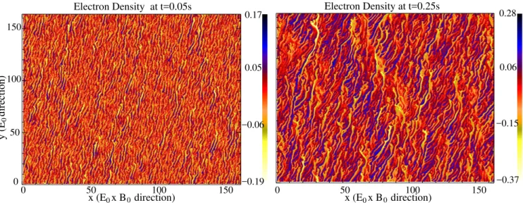
Fig. 1. Plasma density as a function of position at two different times. The color bar to the right indicates the ion density perturbation amplitude. Note that the maximum values of the density perturbation,δnireflect approximately four times the RMS value ofδnibecause of

statistical variations on large meshes.

of reference wherexˆpoints in theE₀_×B₀_direction,_y_ˆ_along E_{0, and}z_ˆalongB_0.

This simulated density evolves from an initial state of white noise through a linear growth stage to a turbulently sat-urated final state. Figure 1 shows the density at two times in this evolution, the first shortly before saturation and the last well into saturation. During the evolution many processes occur, from the initial anisotropic heating of the ions and electrons to cascade processes which couple energy across many scales. By comparing many simulations, we will de-scribe the dominant processes involved in saturation. While the details of how these simulations evolve depends on the parameters, qualitatively all runs show essentially the same behavior as our baseline case.

Tracking electrons as they gyrate dominates the computa-tional cost of these simulations. To reduce this expense, we use an electron mass which is 44 times more massive than the physical electron mass, making the ion to electron mass ratio close to that found in a H+plasma. Our theoretical analysis says that one can raise the electron mass without substan-tially impacting this system until the point where electron Landau damping becomes important, at about 80me. We

performed a test to demonstrate that this elevated electron mass has little effect on these simulations. We ran the base-line case withmsim_e =6me. This run showed no appreciable

changes from the baseline case, showing the same growth rate, saturation amplitudes, and dominant modes. As we reduce the electron mass, we also reduce the frequency of updating the ion velocities and positions. This allows us to increase the number of PIC ions (not changing the density) without increasing the computational cost. The increased number of ions reduces the level of particle noise, allowing

Table 1. Parameters of Baseline Simulation. Here9≡νeνi/ ei

andNepic,N_ipicare the number of macro PIC particles used to model

the behavior of then0nxdxnydyparticles per length. TheTnis the

neutral temperature. All other parameters have their typical mean-ings.

Parameter Value Units

grid span (nx×ny) 1024×1024

grid size (dx×dy) 0.04×0.04 m

1t 4×10−7 s

B₀ 0.5zˆ Gauss

E₀ ₀_.₀₅₀yˆ V/m

n0 1×109 1/m−3

mi 5×10−26 kg

mi/me 1250

νe 2700 1/s

νi 1675 1/s

9 0.14

Tn 300 K

Nepic 2.56×108

N_ipic 2.56×108

us to reduce the number of PIC electrons. This reduction in electron number mitigates the computational cost of reducing the electron mass.

We also ran one simulation which was sixteen times as large as our baseline simulation (4096×4096 grid cells with

(4)

Max and Avg

2

E

2

(V/m)

E2

time (s)

0.00 0.05 0.10 0.15 0.20 0.25

1.0000

0.1000

0.0100

0.0010

0.0001

D0 D1 Perturbed density Max and Avg

0.5

0.4

0.3

0.2

0.1

0.0

0.00 0.05 0.10 _0.15 0.20 0.25

time (s)

|den/n0|

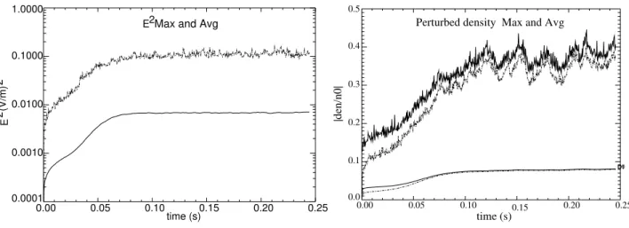
Fig. 2.Electric field energy and density perturbation maximum and average from baseline simulation. Left image shows the time evolution of the maximum (top) line and averaged electric field squared in (V/m)2. Right image shows the evolution of the maximum (top lines) and RMS of the perturbed density (bottom lines). The electron densities are shown with solid lines while ion densities with dashed lines. The base-line noise level of the simulation can be assessed from 10 ms to 25 ms.

at Boston University. We will show images from this large run when appropriate.

4.2 Saturation amplitude

The average perturbation electric field amplitude, hE2i1/2 gives information on the nature of the turbulence. Fig-ure 2a shows that the average field reaches 0.08 V/m for the 4096×4096 run. This exceeds the driving electric field of 0.05 V/m by 60%. For the 1024×1024 baseline run with the same parameters, the rms electric field reached a more mod-est 0.05 mV/m, only 25% above the driving field. It remained the same for the run with the more realistic ion/electron mass ratio. This high rms field is a common feature of 2-D kinetic simulations of the FB instability.

The 12% maximum density perturbation seen in Fig. 2 arises from the PIC noise throughout the mesh. Since we have 16 million cells, this maximum should reach approxi-mately 4 times the RMS particle noise level. The RMS value is a far better indicator of the actual noise. The difference be-tween the maximum electron and ion densities results from using 8 times as many PIC particles to model ion than elec-tron dynamics. We do this because the slow ions iterate only once for every 32 electron timesteps and, hence, we use 8 times as many ions at little computational cost. Despite this difference in maximum values, the system remains highly quasineutral and the saturated electron and ion RMS densi-ties track each other well.

ThehE2i1/2 _{value reflects the combination of the} turbu-lent electric field plus that resulting from individual particle noise. In EPPIC, the ions are cycled less frequently than the electrons since the ions do not need to resolve the electron cyclotron frequency. The ions need a time step which re-solves ion time scales such as the ion acoustic frequency, the

ion plasma frequency, and the ion collision rate. The electric field applied to the ions is the field averaged over the inter-vening electron time-steps. Therefore, the ions experience a less noisy electric field than do the electrons. Because the ions time step is much slower than the electron time step, the number of PIC-particles representing the ion density can be increased without substantial computational expense.

The averaged density perturbation of the turbulent plasma can be compared to the perturbation amplitude of the electric field, theoretical estimates, and in-situ measure-ments by rockets. Figure 2b shows the time evolution of the peak plasma density reached as well as the averaged,

R

(n−n0)2/n2₀dx. From these simulations, we estimate that the saturated average density perturbations is ∼12% while the initial, non-turbulent perturbation is∼2.5%. The maxi-mum density perturbation is typically∼40% while the pre-disturbance perturbation level is∼12%.

Examining these perturbation levels for a series of simu-lations with different electric field drivers should reveal the relationship between this driver and the perturbation ampli-tudes. Figure 3 shows the average electric field amplitude. One sees that the RMS electric field exceedsE₀_{by 20% to} greater than 50% where the higher driving fields cause the greater excesses. The RMS density perturbations start at a modest 6% and rise to 40%. The RMS electric field does not change as a function of electron mass.

(5)

Comparisons of Average Saturated Electric Field

0.04 0.06 0.08 0.10 0.12 0.14 E0 (V/m)

0.00 0.05 0.10 0.15 0.20 0.25

<E> (V/m)

Comparisons of Average Perturbed Saturated Density

0.04 0.06 0.08 0.10 0.12 0.14 E0 (V/m)

0 5 10 15 20

avg. perturbed density (%)

Fig. 3.Saturated RMS electric field and density perturbation levels from four simulations. Left image shows the RMS electric field while the right image shows the RMS of the perturbed density versus driving electric field. Note that the label of the left image,hEirepresents

hE2i1/2.

4.3 Spectra of the saturated system

Radar data typically probes 1 or a few wavevectors of the system with sensitivity to the phase velocity of those waves. Rockets can measure many wavelengths in-situ for a limited time and at a single moving point. Both these measurements gather spectral data which we plan to compare to the simula-tion spectra.

Spectra from two spatial dimensions plus time such as density, ni(x, y, t ), form 3-D spectra, ni(kx, ky, ω), which

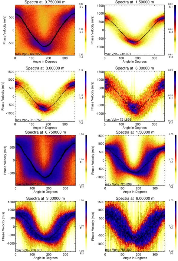
are challenging to display. One can show cross sections or various averages of the data. We will present a number of these as we attempt to extract the most pertinent information. Radars typically measure electrojet waves at a single wavelength but frequently from a number of directions. For comparison purposes, we will show analogous information generated from these simulations. Figure 5 shows the spec-tral information from the 4096×4096 simulation for 4 wave-lengths (i.e.|k|values). We can see from these spectra that the phase velocity changes roughly as a cos(θ−φ) relation-ship whereφis the angle of the phase shift due to the turn-ing of the wave. This turnturn-ing results from a modification of the linear FB relationship due to thermal effects, mostly ion heating (Oppenheim and Dimant, 2004). One can also see this turning in the density images of Fig. 1. One sees from the top 4 images of Fig. 5 that the largest amplitude signal will return from nearly in theE×B _{direction and will fall} off as one measures in the direction perpendicular to this. The power falls off more rapidly for modes near from the dominant, linearly growing, wavelength (∼1.5 m) then for longer or shorter wavelengths. While the cosine relationship of phase velocity agrees with the results of Woodman and Chau (2002), the fall off in energy may not.

0 2 4 6 8

kx

−6 −4 −2 0 2 4 6

ky

0.24 E−4 0.24

E−3 0.24

E−2

0 2 4 6 8

kx

0.17 E−3 0.17 E−2 0.17 E−1

First Quarter Last Quarter

Fig. 4. Spectra showing theRt1

t0 ni(kx, ky, t )dt for the first fourth

of the simulation (t0=0, t1=tfinal/4)and the last fourth (t0=tfinal∗

3/4, t1=tfinal). The logarithmic scale tends to deemphasize the

strongest modes which in the right image are at small values ofk.

To illustrate the average behavior of these simulations, we show the time averaged spatial spectra from the first quar-ter of the simulation and the last quarquar-ter of the simulation in Fig. 4. One sees from these the downward tilt of the waves and how the system evolves from having predomi-nantly short wavelength modes as one would expect from linear kinetic theory to longer waves distributed inhomoge-neously but smoothly through k_{-space. When we look at} animations of(kx, ky)evolving in time, we see a group of

(6)

0 100 200 300 Angle in Degrees -500

0 500

Phase Velocity (m/s)

Spectra at 0.750000 m

0.32 E-4 0.32 E-3 0.32 E-2

max Vph= 660.358

0 100 200 300

Angle in Degrees -1000

-500 0 500 1000 1500

0.61 E-3 0.61 E-2 0.61 E-1

max Vph= 712.021

0 100 200 300

-500 0 500 1000 1500

0.17 E-2 0.17 E-1 0.17

max Vph= 713.752

0 100 200 300

-500 0 500 1000 1500

0.20 E-2 0.20 E-1 0.20

max Vph= 751.856

0 100 200 300

0 500

1.00 E-2 1.00 E-1 1.00

max Vph= 687.881

0 100 200 300

-500 0 500 1000 1500

1.00 E-2 1.00 E-1 1.00

max Vph= 726.899

0 100 200 300

-500 0 500 1000 1500

1.00 E-2 1.00 E-1 1.00

max Vph= 726.981

0 100 200 300

-500 0 500 1000 1500

1.00 E-2 1.00 E-1 1.00

max Vph= 758.330

Fig. 5.Spectra comparingvph=ω/|k|to angle with respect to theE0×B0direction for four wavelengths. The top four figures indicate the

strength of the signal with the color bar to the right of the image. The bottom four normalize the amplitude of the signal at each angle to the maximum signal strength at that angle, in order to better compare with radar data which generally show normalized spectral amplitudes. The curve drawn through the signal is the moment of the signal at each angle and this indicates the mean phase velocity. The peak value ofvph

(7)

0.00 0.05 0.10 0.15 0.20 0.25

time (s)

300 320 340 360 380 400

420 <Vx^2>

<Vy^2>

<vz^2>

0.00 0.05 0.10 0.15 0.20 0.25 300

305 310 315 320 325

<Vx^2> <Vy^2>

<Vz^2>

Electron Thermal Energies

Energy (K)

Ion Thermal Energies

Fig. 6.Electron and ion thermal energy of large baseline simulation. These are expressed asmhv_j2i/Kbwherejis the direction unit vector,

mis the species mass andKbis the Boltzmann constant. The temperatures rise from 300 K, initially because of frictional heating due to

E0yˆ, and further due to wave heating. Our predicted electron and ion temperatures are very similar to those that develop in the simulations.

Note that these simulations includevzvalues for each particle. These values change only because collisions with neutrals slowly make the

distributions more isotropic (noEzexist).

The peak velocity is also listed on each frame of the figure. This velocity exceeds the acoustic speed of the system if one calculates that speed using the temperature of the neutrals and for isothermal electrons and ions,Csn=407 m/s.

How-ever, neither species is truly isothermal, nor do they remain at the neutral temperature of 300 K. Figure 6 shows the tem-perature evolution of the large baseline simulation. If we adjust for the enhanced temperature and assume the elec-trons are fully adiabatic while the ions are isothermal, then

Cs≈500 m/s. While these assumptions are not precisely

cor-rect, a dramatically higher acoustic speed seems incorrect. For short wavelengths, the ions will not have time to fully isotropize during a wave cycle. If the ions behaved as a fully 3-D adiabatic gas thenCs≈550 m/s, while if they were a 1-D adiabatic gas thenCs≈650 m/s. In all cases, these peak

velocities remain well below the velocity predicted by lin-ear theory,Vd/(1+9)=950 m/s. We will analyze the phase

velocities more completely in the discussion section. If these simulations were fully 3-D, we would expect the electron temperatures to rise more dramatically as electrons accelerate due to the small wave-driven parallel electric field. Even in a 2-D simulation with noE||, the moments of the electron distribution increases because of wave induced com-pression and inelastic collisions between electrons and neu-trals (see Dimant and Oppenheim, 2004, for more details).

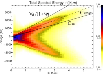
To examine phase velocity over a range of wavelengths, we can compare the wave frequency,ω, from the saturated component of the simulation to wave number,|k|. Figure 7 shows these spectra. Clearly most of the energy falls within the acoustic modes with a∼700 m/s velocity. One can also see that there is substantial spectral broadening, particularly at low k. At high k, the acoustic speed may increase as

0 1 2 3 4 5

|k| (1/m) −2000

−1000

−3000 0 2000

1000 3000

omega (1/s)

Total Spectral Energy: n(|k|,w)

0.26 E−4 0.26 E−3 0.26 E−2

C

d

V /(1+ )

_Ψ

C

smax

sa

Fig. 7. Power as a function of|k|and ω. This is generated by summing over all the angles from spectra like those seen in Fig. 5. Lines forCsa=500 m/s,Vd/(1+9)=950 m/s andCsmax=650 m/s

(dashed) have been placed on the figure for reference.

the ions become more adiabatic. For fully adiabatic 1-D ions (γi=3) and 3-D electrons (γe=5/3),Csbecomes almost

650 m/s which appears to match the phase velocities of these shorter modes (k>2).

4.4 Spectral content

(8)

0 100 200 300 Angle in Degrees 0

100 200 300 400 500 600

0 100 200 300

Angle in Degrees

1.5 m wavelength waves 3.0 m wavelength waves 6.0 m wavelength waves

0 100 200 300

0 200 400 600 800 1000

Angle in Degrees 0

100 200 300 400 500

spectral width (m/s)

Fig. 8. Spectral widths for 3 different wavelengths (|k|) as a function of angle. The black lines show the second moments of the spectral information displayed in Fig. 5. The red lines show the standard deviation of a Gaussian fit to the spectra and gives a better representation of the spectral width.

0.0001

k (1/m)

0 5 10 15

0.01

n(k)

1.0

0.1

0.001

Max and Avg Spectral density

Max

Avg

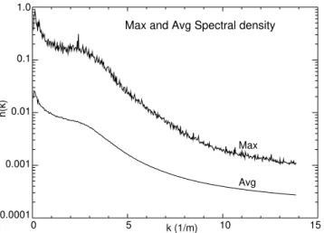
Fig. 9. Power as a function of|k|and ω. This is generated by summing over all the angles from spectra like those seen in Fig. 5. The “max” curve shows then(|k|, ω)with the highestωwhile the “avg” curve averagesn(|k|, ω)over allω.

angles from the largest simulation. We generate these using two methods. The first mode takes the second moment of

n(|k|, ω)for a givenk,

vw =

s R∞

−∞n(|k|, ω)(ω−ω0)2dω

n(|k|)|k|2 (1)

where ω0 is the first moment of n(|k|, ω) and

n(|k|)=R∞

−∞n(|k|, ω)dω is the normalization factor.

Since low amplitude noise at large velocities can cause the second moment to become dramatically larger than one would obtain if the noise level were lower, we also fitted n(k, ω) to the sum of a Gaussian plus a quadratic polynomial. The standard deviation of the fitted Gaussian gives a better representation of the spectral width. One sees that the simulation generates substantial spectral broadening

in all directions and at all wavelengths. The spectrum is narrowest where it is strongest, in the direction of greatest linear growth, and broadest perpendicular to that direction. Shorter wavelengths have less spectral broadening but the difference between 1.5 and 6 m modes is less than a factor of two.

Rockets generate a spectrum by comparingktoωfor the time-series data they collect. Simulations can generate sim-ilar spectral information. Figure 9 shows such a comparison generated by Fourier transforming theni(x, y, t )array from

the saturated part of the simulation into ani(kx, ky, ω)

ar-ray. We then interpolate along paths of fixed|k| to obtain ani(|k|, ω)array. We then find the maximum and average

values of these arrays and plot them to make Fig. 9. Making a direct comparison between these simulation results and the rocket spectrum will require substantial further analysis.

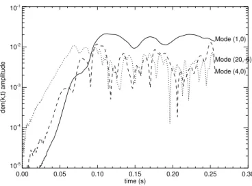
These simulations all show energy flowing into longest horizontal waves which the simulation supports. For the 4096×4096 simulation, this means that energy flows into waves with wavelengths approaching 160 m. This mode eventually becomes the dominant mode in the system. Fig-ure 10 compares the growth of the longest mode to one of the dominant linearly driven modes from the baseline sim-ulation. One can see that the longer mode develops much later than the shorter one. However, its growth rate is similar or faster than the shorter mode. For long wavelengths, the predicted linear growth rate is proportional tok2, so that, if linear growth were the cause of the long wavelength modes growth, we would expect this mode to grow at 1/436 the speed of the longer mode (neglecting kinetic reduction of the short wavelength growth rate). The 40 m wave (dashed line) also grows at the same rate as the 160 m wave, implying that these are not linear FB growth processes, but instead result from coupling to shorter modes.

(9)

Waves which span the entire simulation model cannot satu-rate in the same way since they cannot couple to longer waves nor can they smoothly turn since the simulation does not sup-port a broad spectrum of waves at such long wavelengths. These longer waves can saturate through a alternate mecha-nisms including coupling to shorter wavelengths or particle heating. We are not certain of the mechanism.

5 Discussion and conclusions

These simulations show the nonlinear behavior of saturated FB waves in 2-D. While one can modify the parameters to change the driving field and the effective altitude, these changes do not dramatically impact the qualitative behavior of the waves. This is because the waves dissipate their energy by coupling to other modes both at longer and similar wave-lengths. In this section, we briefly discuss some interesting features of the saturated FB waves found in our 2-D sim-ulations, estimate basic quantitative characteristics of these waves, and compare our estimates with these simulation re-sults.

The most intriguing feature of our simulations is the trans-fer of turbulent energy from short-wavelength waves (pre-ferred by the linear instability growth rates) to much longer waves. In the saturated state, the maximum of turbulent en-ergy always shifts toward the longest waves allowed by the simulation box size. As we increase our box size, not only does the most energetic wave become longer but the rms tur-bulent electric field becomes larger. In the real electrojet, the 3-D geometry and natural gradients of the background medium may impose a preferred maximum wavelength.

What physical mechanism causes inverse cascading from short to long wavelength? For long wavelengths the linear instability growth rate scales as the wavenumber squared,

γ∝k2. If one waits long enough, one would expect long wavelengths to develop. However, in the simulations these waves develop much faster than predicted by the linear the-ory, suggesting that nonlinear mode-coupling plays a crucial role in their development through an inverse cascade mecha-nism. We do not yet have a model explaining this aspect of the simulations.

We ran these simulations with a range of driving electric fields, E₀ _{and found that the threshold} elec-tric field necessary to generate instabilities is nearly twice the minimum isothermal fluid-model value,

EThr=[(Te+Ti) /mi]1/2B0(1+9)≈23 mV/m (for the undisturbed temperaturesTe0=Ti0=Tn=300 K,mi≈30 amu,

andB0=0.5×105nT). There may be several reasons for the discrepancy. First, the driving field itself heats both electrons and ions, increasing the threshold. In our simulations, however, this initial heating was fairly small, ∼10−20 K for each species. Second, the small charge separation between electrons and ions, disregarded in quasineutral fluid theory, can also increase the threshold field by a factor

0.00 0.05 0.10 0.15 0.20 0.25 0.30 time (s)

10-5

10-4

10-3

10-2

10-1

den(k,t) amplitude

Mode (1,0)

Mode (4,0) Mode (20,-6)

Fig. 10. ni(k, t )vs. time for two modes, the solid line shows the

(1,0) mode which is atk=(2π/41,0)m−1, the dotted line shows the (20,−6) mode atk=(2π/2.0,2π/6.8)m−1and the dashed line shows the (4,0) mode.

of (1−ν_i2/ω2_pi)−1/2=(1−ncr/n0)−1/2, where ωpi is the

ion plasma frequency and the critical density is given by

ncr=miν_i2ǫ0/e2≈4.84×107m−3 (Rosenberg and Chow, 1998). In our simulations, we had(1−ncr/n0)−1/2≈1.05, so that this factor should not play an important role. Third, and most importantly, the non-isothermal and kinetic behavior of plasma appears to substantially elevate the instability threshold. If both electrons and ions behaved adiabatically, this would increase the threshold value by a factor of

γe1/2=γ_i1/2=(5/3)1/2≈1.29. In these collision-dominated,

low-frequency, E-region processes, however, the situation is more complex and neither the electrons nor ions behave a simple adiabatic or isothermal fluid. This is also true in these simulations as discussed below.

Both ion and electron thermal behaviors modify the in-stability threshold. The simplified fluid-model analysis in Dimant and Oppenheim (2004) shows how ion thermal ef-fects cause the predominant F-B waves to travel in a dif-ferent direction fromE₀×B_{0-drift velocity but impacts the} instability threshold only a little. Electron thermal factors calculated using both kinetic and fluid models give a cor-rected value of electron adiabatic indexγe which will raise

the threshold substantially (Dimant and Sudan, 1995a,b; Kagan and St.-Maurice, 2004). In these simulations, we modeled electron-neutral collisions using an elastic hard-sphere interaction module which gives a kinetic collision fre-quency proportional to the electron velocity. We matched the inelastic collision and heat transfer rates by colliding the electrons with a reduced mass neutral species. Us-ing Eqs. (61) to (64) from Dimant and Sudan (1995b) withα=1/2 andx=0, we obtain γe=1+Pω,k≈2.58. This

(10)

wavelengths, the kinetic effects of ion Landau damping in-creases the threshold drastically. Note that for the longer wavelengths – the ones that dominate these simulations – where(2me/m∗n)νi≪ω−kV0, we expect electron cooling to

reduceγewhich will decrease the threshold. The

combina-tion of all listed factors can increase the threshold by a factor somewhat less that 2, though there may be some additional unidentified factors. Also, bear in mind that it is difficult to determine the exact value of the threshold electric field from simulations because small instability growth rates close to the threshold require long times for the instability to develop. Finally, fluctuation noise associated with the finite number of PIC particles can preclude the measurement of waves driven near their instability threshold, though with these massively parallel simulations, we can drive that noise down to a frac-tion of a percent.

Figure 6 shows that heating occurs in a two-step process for both electrons and ions. The initial heating stage results from the frictional heating caused by the driving electric field itself. Then, after several tens of milliseconds, the wave elec-tric field causes additional heating. Equation (34) from Di-mant and Milikh (2003) predicts an initial heating for ions of≃12 K which agrees reasonably well with the anisotropic temperature increases of 20 K for hVyi and 11K for hVxi

andhVzi. The anisotropy occurs because the ion Pedersen

drift velocity (vPed≃95 m/s) is nearly one third of the mean thermal speed defined by vT i=(Ti/mi)1/2. In the

highly-collisional regime, whenvPed is not small compared with

vT i, the distribution function can easily deviate from a simple

Maxwellian and become anisotropic.

The electron velocity distribution is much more isotropic than that of ions because both collisions of light low-energy electrons with heavy neutrals results mainly in an-gular scattering and relatively slow energy changes. The energy exchange rate (δen in Dimant and Oppenheim

(2004)) has been modeled in our code by an artificially re-duced neutral mass, m∗, so that in our baseline simula-tion δen=2me/m∗n≈8×10−2 (this value exceeds the actual

E-region values by one to two orders of magnitude but com-pensates appropriately for the artificially massive electrons). Using Eq. (37) from Dimant and Milikh (2003), we ob-tain Ti−T0≃25 K, which agrees well with the initial elec-tron heating. The characteristic times of this initial heating,

(δenνe)−1≃5 ms for electrons andν_i−1≃0.6 ms for ions also

agree well with the observed times of the initial heating, as seen in Fig. 6.

The 2-D turbulent heating level can be estimated from the same formulas using the rms values of the turbulent electric fieldhEi instead ofE_{0. According to Fig. 2,}hEi reaches 84 mV/m, which yields an estimate for the final electron heating of≃95 K and for ions≃45 K. These estimates give a slightly lower value for electron temperature and exaggerate significantly ion heating. This may be due to oversimplifica-tion of the fricoversimplifica-tional heating model in the theory which does not account for deviations from Maxwellian distributions or

the rather large ratio of the drift velocity to the thermal speed. Note that the rms turbulent electric field in these simulations was larger than one would expect from simple heuristic rea-sonings and larger than those observed by rockets. We hope that 3-D simulations will reduce the rms field value because the third dimension creates an important degree of freedom for instability saturation.

These heating effects may help explain the elevated value of the wave phase velocity compared to the cold-plasma ion-acoustic speed. Using the final elevated temperatures along with kinetically calculated γe, as we did above,

we can easily obtain a renormalized ion-acoustic speed of

Cs≃700−750 m/s. Assuming that most energetic waves

set-tle on the margin of linear stability for,Vph≈Cs, we obtain

the peak values listed on Fig. 5. A more accurate analysis is needed, but even these simple estimates show that a con-ventional assumption of peakVph≈Cs with the underlying

reasonings do not contradict our 2-D simulations.

The principle limitation on these results arises from the simulations being only 2-D. We expect to address this and further analyze these 2-D results in future papers.

Acknowledgements. Topical Editor M. Pinnock thanks two anony-mous referees for their help in evaluating this paper.

References

Bahcivan, H. and Hysell, D. L.: A model of secondary Farley-Buneman waves in the auroral electrojet, J. Geophys. Res. (Space Physics), 111, 1304, doi:10.1029/2005JA011408, 2006. Bowles, K. L.: Doppler-shifted radio echoes from aurora, J.

Geo-phys. Res., 59, 553, 1954.

Dimant, Y. S.: Nonlinearly Saturated Dynamical State of a Three-Wave Mode-Coupled Dissipative System with Linear Instability, Phys. Rev. Lett., 84, 622–625, 2000.

Dimant, Y. S. and Milikh, G. M.: Model of anomalous electron heating in the E region: 1. Basic theory, J. Geophys. Res., 108, 5–1, 2003.

Dimant, Y. S. and Oppenheim, M. M.: Ion Thermal Effects on E-Region Instabilities: Linear Theory, J. Atmos. Solar Terr. Phys., 66, 1655–1668, 2004.

Dimant, Y. S. and Sudan, R. N.: Kinetic Theory of the Farley-Buneman Instability in theEregion of the Ionosphere, J. Geo-phys. Res., 100, 14 605–14 624, 1995a.

Dimant, Y. S. and Sudan, R. N.: Kinetic theory of low-frequency cross-field instability in a weakly ionized plasma. I, Phys. Plas-mas, 2, 1157–1168, 1995b.

Dyrud, L., Krane, B., Oppenheim, M., P´ecseli, H. L., Schlegel, K., Trulsen, J., and Wernik, A. W.: Low-frequency electrostatic waves in the ionospheric E-region: a comparison of rocket ob-servations and numerical simulations, Ann. Geophys., 24, 2959– 2979, 2006,

http://www.ann-geophys.net/24/2959/2006/.

(11)

Fejer, B. G., Providakes, J., and Farley, D. T.: Theory of plasma waves in the auroral E region, J. Geophys. Res., 89, 7487–7494, 1984.

Fontenla, J. M.: Chromospheric plasma and the Farley-Buneman instability in solar magnetic regions, Astron. Astro., 442, 1099– 1103, doi:10.1051/0004-6361:20053669, 2005.

Haldoupis, C., Ogawa, T., Schlegel, K., Koehler, J. A., and Ono, T.: Is there a plasma density gradient role on the generation of short-scale Farley-Buneman waves?, Ann. Geophys., 23, 3323–3337, 2005,

Hamza, A. M. and St.-Maurice, J. P.: A turbulent theoretical frame-work for the study of current-driven E region irregularities at high latitudes: basic derivation and application to gradient-free situa-tions, J. Geophys. Res., 98, 11 587–11 599, 1993.

Hysell, D. L. and Drexler, J.: Polarization of elliptic E re-gion plasma irregularities and implications for coherent radar backscatter from Farley-Buneman waves, Radio Sci., 41, 4015, doi:10.1029/2005RS003424, 2006.

Hysell, D. L., Drexler, J., Shume, E. B., Chau, J. L., Scipion, D. E., Vlasov, M., Cuevas, R., and Heinselman, C.: Combined radar observations of equatorial electrojet irregularities at Jicamarca, Ann. Geophys., 25, 457–473, 2007,

Kagan, L. M. and St.-Maurice, J.-P.: Impact of electron ther-mal effects on Farley-Buneman waves at arbitrary aspect an-gles, J. Geophys. Res. (Space Physics), 109, 12 302, doi:10.1029/ 2004JA010444, 2004.

Kelley, M. C.: The Earth’s Ionosphere, Academic, San Diego, Calif., 1989.

Oppenheim, M. M. and Dimant, Y. S.: Ion Thermal Effects on E-Region Instabilities: 2-D Kinetic Simulations, J. Atmos. Solar Terr. Phys., 66, 1639–1654, 2004.

Oppenheim, M. M., Otani, N. F., and Ronchi, C.: Saturation of the Farley-Buneman instability via nonlinear electronE×B drifts, J. Geophys. Res., 101, 17 273–17 286, 1996.

Otani, N. F. and Oppenheim, M.: Saturation of the Farley-Buneman instability via three-mode coupling, J. Geophys. Res. (Space Physics), 111, 3302, doi:10.1029/2005JA011215, 2006. Rosenberg, M. and Chow, V. W.: Farley-Buneman instability in a

dusty plasma, Planet. Space Sci., 46, 103–108, 1998.

Sahr, J. D. and Farley, D. T.: Three-wave coupling in the auroral E-region, Ann. Geophys., 13, 38–44, 1995,

St.-Maurice, J.-P. and Hamza, A. M.: A new nonlinear approach to the theory of E region irregularities, J. Geophys. Res., 106, 1751–1760, 2001.