Bottom-trawling fisheries influence on standing stocks, composition, diversity and trophic redundancy of macrofaunal assemblages from the West Iberian Margin

Author’s Accepted Manuscript

Bottom-trawling fisheries influence on standing

stocks,

composition,

diversity

and

trophic

redundancy of macrofaunal assemblages from the

West Iberian Margin

Sofia Pinto Ramalho, Mariana Almeida, Patricia

Esquete, Luciana Génio, Ascensão Ravara, Clara

F. Rodrigues, Nikolaos Lampadariou, Ann

Vanreusel, Marina R. Cunha

PII:

S0967-0637(18)30001-3

DOI:

https://doi.org/10.1016/j.dsr.2018.06.004

Reference:

DSRI2921

To appear in:

Deep-Sea Research Part I

Received date: 5 January 2018

Revised date:

16 May 2018

Accepted date: 8 June 2018

Cite this article as: Sofia Pinto Ramalho, Mariana Almeida, Patricia Esquete,

Luciana Génio, Ascensão Ravara, Clara F. Rodrigues, Nikolaos Lampadariou,

Ann Vanreusel and Marina R. Cunha, Bottom-trawling fisheries influence on

standing stocks, composition, diversity and trophic redundancy of macrofaunal

assemblages from the West Iberian Margin,

Deep-Sea Research Part I,

https://doi.org/10.1016/j.dsr.2018.06.004

This is a PDF file of an unedited manuscript that has been accepted for

publication. As a service to our customers we are providing this early version of

the manuscript. The manuscript will undergo copyediting, typesetting, and

review of the resulting galley proof before it is published in its final citable form.

Please note that during the production process errors may be discovered which

could affect the content, and all legal disclaimers that apply to the journal pertain.

Bottom-trawling fisheries influence on standing stocks, composition,

diversity and trophic redundancy of macrofaunal assemblages from the West

Iberian Margin

Sofia Pinto Ramalho1,2*, Mariana Almeida1, Patricia Esquete1, Luciana Génio1, Ascensão Ravara1, Clara F. Rodrigues1, Nikolaos Lampadariou3, Ann Vanreusel2, Marina R. Cunha1 1_{Departamento de Biologia, Universidade de Aveiro, Campus Universitário de Santiago,}

3810-193 Aveiro, Portugal

2_{Department of Biology, Marine Biology Research Group, Ghent University, Krijgslaan} 281/S8, 9000 Ghent, Belgium

3_{Hellenic Centre for Marine Research, Institute of Oceanography, P.O. Box 2214, 71003,} Heraklion, Crete, Greece

Email address: sofia.pinto.ramalho@gmail.com; sramalho@ua.pt

*Corresponding author: Sofia P. Ramalho

Abstract

Bottom-trawling fisheries operating in Portugal (West Iberian Margin) impose one of the largest footprints per unit of biomass landed in European waters at depths greater than 200 m, affecting the seafloor integrity and the associated benthic fauna. To investigate how trawling pressure is affecting the macrofaunal assemblages, we compared the standing stock (abundance and biomass), community structure and taxonomical and trophic diversity in areas subjected to varying trawling pressure along the SW Portuguese upper slope, between 200-600 m. In addition to trawling pressure, several environmental variables, namely depth, grain size and organic matter, were correlated with the biological component, which suggest that the longstanding trawling pressure presents cumulative effects to the habitat heterogeneity known to characterise the West Iberian Margin fauna. Furthermore, our results showed a depletion of macro-infaunal abundances in both the fishing ground and the adjacent area (up to 3 times lower), when compared to the area not trawled. The observed decrease in abundance with increasing trawling pressure was also associated with a loss of species and trophic richness, but univariate diversity indices

related with community structure (i.e. Shannon-Wiener index, Pielou’s evenness) failed to detect consistent differences across areas. Also observed was a decrease in the number of taxa - trophic guilds combinations of the core assemblage (i.e. characteristic, dominant or frequent taxa) with increasing trawling pressure. We suggest that, in disturbed sediments, the lower functional redundancy resulting from the loss of species within most feeding guilds increases the vulnerability of trophic interactions and therefore of the whole assemblage to further increases in natural and anthropogenic disturbance or their synergistic effects.

Keywords: macrobenthos; diversity; physical disturbance; bottom-trawling fisheries; deep

sea.

1. Introduction

The increased awareness on the putative impacts of bottom-trawling fisheries has promoted research on marine biodiversity and ecosystem functioning alterations particularly in continental shelf areas (Jennings and Kaiser, 1998; Kaiser et al., 2002; NRC, 2002; Tillin et al., 2006; Mangano et al., 2013; Bolam et al., 2014; Mangano et al., 2014; Sciberras et al., 2018). The magnitude of bottom-trawling pressure depends chiefly on the gear type and the spatial and temporal scales associated with trawling (NRC, 2002; Hiddink et al., 2017; Sciberras et al., 2018). On the other hand, the resistance (capacity to resist change) and resilience (capacity to recover from change) of the ecosystem is largely determined by the life history traits of the inhabiting fauna (e.g. reproductive and dispersal capacity), the characteristics of the targeted habitats (including depth) and their regional setting (biogeography, latitude, connectivity with similar, non-impacted habitats) (Clark et al., 2015; van Denderen et al., 2015; Lambert et al., 2017). Known direct effects associated with trawling fisheries include: i) mortality of both target and non-target populations; ii) increased food availability for both predators and scavengers owing to discarding practices and on-site faunal mortality or injury; and iii) alterations or even loss of habitat complexity – e.g. sediment reworking and loss of habitat-forming fauna (NRC, 2002; Thrush and Dayton, 2002; Hiddink et al., 2006; Mangano et al., 2015). Indirect effects are derived from the former, and may involve long-term changes on infauna standing stocks, shifts in community composition, and eventually weakening food web stability (Jennings et al., 2001a,b; Kaiser et al., 2002; NRC, 2002; Thrush and Dayton,

2002; Duplisea et al., 2002; Pusceddu et al., 2014; van Denderen et al., 2015; Mangano et al., 2017; Hinz et al., 2017). The loss of disturbance-sensitive species, for instance filter-feeding fauna such as sponges, bivalves and polychaetes, is usually observed in highly disturbed areas by trawl fisheries, as these organisms are easily smothered or are unable to efficiently feed during high turbidity periods induced by the re-suspension of sediments during trawl ploughing (Lindeboom and De Groot, 1998; Leys, 2013; Clark et al., 2015; Bastari et al., 2018). Although rare in marine systems, trophic cascading effects due to loss of species were also reported in areas subjected to high intensity and frequent trawling pressure (Pace et al., 1999; Coleman and Williams, 2002; Pauly et al., 2013; Hinz et al., 2017).

Loss of species leads to decreased functional redundancy (number of species within each functional entity) and, ultimately, also decreased complexity of food webs (total number of functional entities and their interactions) (Hooper et al., 2005). Species richness has both a buffering effect (reduces temporal variance) and a performing-enhancing effect on ecosystem functions (Yachi and Loreau, 1999). In general terms, species richness, through compensatory dynamics, ensures the ecosystems against declines in their functions (“the Insurance Hypothesis”) and it is a critical feature to the reliability of ecosystems functioning and their long-term capacity to provide goods and services (Naeem and Li, 1997; Naeem, 1998). There is theoretical and accumulating empirical evidence (Liu et al., 2016, and references therein) that this compensatory dynamics may also limit the strength of trophic cascades (designated by Frank et al. (2006), as “Community Regulation Hypothesis”); it increases food web connectance by promoting additional interactions among (e.g. omnivory) and within trophic guilds (e.g. competition, intraguild predation) and diffuses the direct effects of consumption and productivity throughout the trophic spectrum (Frank et al., 2006). Trophic cascades are generally believed to be less frequent and weaker in functional redundant detritus-based food webs that deviate from a linear food chain (Liu et al., 2016).

High diversity has also been related with greater stability, resistance and resilience of ecosystems (Strong et al., 2015, and references therein). However, high diversity, or even functional redundancy, per se does not ensure resilience, because the replacement of local extinctions in disturbed systems depends on the probability of recolonization from adjacent habitats and/or from a regional pool of species (Naeem; 1998). More importantly, the relationship between diversity and stability is a complex problem that cannot be understood outside the context of the environmental drivers (e.g., climate, resource availability, and natural disturbance (Ives and Carpenter, 2007)). Additionally, human

activities can modify and act synergistically with all of these drivers (Hooper et al., 2005). In Portuguese waters, the estimates of seabed integrity indices for bottom-trawling practices (including all types of bottom-contact gears) are among the lowest in European waters, resultant from both the large footprint per unit of landing (ca. 17 km2.t-1) and large total area trawled annually (93.6%) below 200 m water depths (Eigaard et al., 2016), which expresses the enormous pressure imposed by trawling to these deep-sea benthic habitats. The need to ensure the sustainable functioning of ecosystems is acknowledged by marine policy requirements such as the European Marine Strategy Framework Directive (MSFD) 2008/56/EU (European Commission, 2008). Yet, our understanding of the effects of trawling practices on deep-sea benthic ecosystems in Portugal, is still very limited and predominantly restricted to studies on large-sized mega-epifauna (Morais et al., 2007; Fonseca et al., 2014), or related with coastal bivalve dredging (Chicharo et al., 2002; Falcão et al., 2003; Gaspar et al., 2003). The MSFD definition of Good Environmental Status (GES) includes the requirement that “the structure, functions and processes of the

constituent marine ecosystems allow those ecosystems to function fully and to maintain their resilience to human-induced environmental change” (European Commission, 2008). However, reference data on benthic assemblages prior to fishing exploitation is often scarce, or even non-existent for deeper habitats, and adequate control areas are difficult to find, hindering a rigorous assessment of the environmental status of the impacted ecosystems. Thus, the present study aims to investigate putative changes in macrofauna assemblages resulting from long-term crustacean bottom trawling at the upper slope of the Southwest Iberian margin. Specifically, we assessed the differences in macrofaunal assemblages from areas subjected to three levels of trawling pressure (not trawled, adjacent area to the fishing ground and the fishing ground) in terms of macrofauna standing stocks (abundance and biomass), community composition, structural and trophic diversity and trophic redundancy. The results were interpreted in relation to the environmental setting of the study area.

2. Materials and Methods

2.1. Study area

The West Iberian margin (WIM) presents complex and diverse geomorphological and hydrographic features (Relvas et al., 2007; Voelker et al., 2009; Maestro et al., 2013; Kämpf and Chapman, 2016). Among the numerous sources of heterogeneity in this region

are various topographic features (submarine canyons, rocky outcrops) and sediment types which interact with several oceanographic processes, such as various water masses and fronts determining spatial and temporal variability in salinity, temperature and oxygen content (Relvas et al., 2007; Kämpf and Chapman, 2016). Periodic and episodic natural disturbance events (e.g. strong near-bottom currents, high energy winter storms) promote the erosion of sediments from the shelf and their transport and deposition into deeper areas (Vitorino et al., 2002; Diogo et al., 2014). Seasonally variable surface productivity regimes (upwelling and downwelling) are responsible for the horizontal and vertical patchiness of particulate organic matter (POC) flux to the seabed in this region (Fiúza, 1983; Kämpf and Chapman, 2016). Typically, the major peaks in surface primary production occur during spring and summer as a consequence of seasonal upwelling events forced by intense northerly winds. During these periods, large phytoplankton blooms reach several kilometres offshore (often 30–40 km but as far as 200-300 km) or are transported along shelf areas through complex circulation patterns. During winter, low productivity regimes are derived from downwelling under south-westerly winds and mixing by strong storm events may occasionally take place (Fiúza, 1983; Relvas et al., 2007; Kämpf and Chapman, 2016). However, pulse episodes of reverse winds can occur during all seasons (Kämpf and Chapman, 2016). By their relevant contribution to total standing stocks and primary production, upwelling events have a significant impact on both pelagic and benthic food webs supporting the productive fisheries along the Iberian western coast (Santos, 2001; Picado et al., 2014).

Bottom-trawling fishery grounds at the WIM are delimited by legal measures that prohibit trawling practices within six nautical miles from the coastline (MAMAOT, 2012). This adds to the narrow shelf and steep slope prompting the concentration of crustacean otter trawlers at the shelf break and upper slope (200–800 m depth), primarily in the South and Southwest regions off Portugal, within soft sediment areas (mud and muddy-sand), the preferred habitat of several targeted species. This métier targets mainly several species of deep-water crustaceans such as the Norway lobster (Nephrops norvegicus), red and rose shrimps (Aristeus antennatus and Parapenaeus longirostris, respectively), but also a few fish species such as the blue whiting (Micromesistius poutassou) and the European hake (Merluccius merluccius) (Campos et al., 2007; Bueno-Pardo et al., 2017). Because this métier is highly unselective, usually results in large rates of by-catch and discarding. Conservative estimates reported that 28-40% of the total catches of crustacean otter trawlers are catch, while more severe estimates have reported up to 70% of by-catch (Borges et al., 2001; Monteiro et al., 2001).

2.2. Sample collection and processing

During the RV Belgica cruises B2013/17 (10/06/2013–18/06/2013) and B2014/15 (02/06/2014–10/06/2014) several stations were selected to investigate macrofauna assemblages and sediment properties from three main areas subjected to different degrees of trawling pressure (TP): not trawled (NT), an adjacent area to the fishing ground (AA) and the main fishing ground (FG). These were chosen based on similar surface sediment composition (muddy-sand sediments; Ramalho et al., 2017) but distinct trawl pressure regimes, from which information was initially obtained from Vessel monitoring systems (VMS) data reports compiled by Direção Geral de Recursos Marinhos (MAMAOT, 2012) and confirmed during ROV video surveys performed within the framework of this project (Ramalho et al., 2017). Additionally, annual trawl pressure estimates (expressed as hours per km2 _{in a year - h.km}-2_.y-1_{) were determined according to Bueno-Pardo et al.} (2017), for individual cells with an area of 0.01 x 0.01 decimal degrees (ca.1.006 km2), based on Vessel monitoring systems (VMS) position data of crustacean bottom otter trawlers operating in the study area, provided by DGRM.

In total, seven stations were sampled on upper continental slope off Sines and near the Setúbal canyon between depths of ca. 200 and 600 m water depth (Fig. 1 and Table 1). Three to four replicates were obtained in each sampling station and classified into a certain trawling pressure area: not trawled (st. 9 and st. 10), adjacent area to fishing ground (st. 2 and st. 6) and the main fishing ground (st. 1, st. 4 and st. 7). Not trawled (NT) label was only assigned to the stations located in an area safeguarded by current legal restrictions and where trawling has not occurred for the past decades (stations in the vicinity of the Setúbal canyon head). Adjacent area to the fishing ground (AA) stations correspond to those that have been undisturbed or only subjected to very few trawl passages in time and space (trawling pressure estimates ranged between 0–1.5 h.km-2.y -1_{), but were located adjacently to the main fishing ground where the highest pressure} estimates were obtained (FG) (Fig. 1 B,C). This AA area presented overall very few and mostly eroded trawl scars during ROV video surveys (Ramalho et al., 2017). Lastly, the fishing ground (FG) stations corresponded to those located in the area where crustacean otter trawlers typically fish (TP estimates greater than 1.5 h.km-2.y-1) and where video surveys detected a relatively high number of trawl scars on the seabed, most apparently recent (Fig. 1 B,C) (Ramalho et al., 2017). The allocation of each station to a certain trawling pressure area was also confirmed with the effort estimates obtained from the

OSPAR Data & Information Management system database for 2014 (expressed as swept area ratio, the area that has been swept in relation to the total seabed area; Fig. A.1 and Table A.1) (OSPAR Data & Information Management System database, 2017). Detailed bottom-trawling fisheries swept area ratio information for 2013 was not available.

Figure 1. (A) Overview of the study area with indication of the sampled stations (3-4 replicates per station) and detailed trawling pressure data (h.km-2_.y-1_{) for the years of (B) 2013 and (C) 2014.}

Trawl pressure information for st. 9 and st. 10 (Setúbal canyon area) is not shown due to null trawling pressure estimates (0 h.km-2_.y-1_{). Red dashed line establishes the legal six nautical miles}

Table 1. Metadata on sampled stations. Trawling pressure area groups include: not trawled (NT); adjacent area to the fishing ground (AA) and fishing ground (FG). Stations are ordered by the increasing average trawling disturbance of the station in each sampling year.

Cruise Station Deployment Area Latitude

(N) Longitude (W) Depth (m) B2013/17 2_13 22 AA_13 37°58'888 09°07'528 335 2_13 23 AA_13 37°58'896 09°07'506 335 2_13 24 AA_13 37°58'894 09°07'514 335 1_13 4 FG_13 37°59'006 09°11'107 445 1_13 8 FG_13 37°58'962 09°11'111 445 1_13 9 FG_13 37°58'948 09°11'099 445 B2014/15 9_14 73 NT_14 38°20'505 09°12'084 329 9_14 72 NT_14 38°19'872 09°11'645 326 9_14 71 NT_14 38°19'426 09°11'150 340 10_14 76 NT_14 38°20'469 09°13'644 360 10_14 75 NT_14 38°19'998 09°13'063 550 10_14 74 NT_14 38°19'475 09°12'530 407 6_14 31 AA_14 37°56'498 09°07'486 323 6_14 32 AA_14 37°56'670 09°07'486 325 6_14 30 AA_14 37°55'590 09°06'997 300 6_14 29 AA_14 37°54'977 09°06'494 285 2_14 66 AA_14 37°59'902 09°07'454 350 2_14 65 AA_14 37°58'969 09°07'480 336 2_14 64 AA_14 37°57'955 09°07'953 342 7_14 28 FG_14 37°48'488 09°05'447 299 7_14 25 FG_14 37°47'598 09°05'496 291 7_14 26 FG_14 37°47'584 09°05'493 290 7_14 27 FG_14 37°46'842 09°05'437 295 4_14 63 FG_14 37°50'952 09°06'523 318 4_14 34 FG_14 37°49'364 09°06'897 330 4_14 33 FG_14 37°47'997 09°06'911 330 1_14 70 FG_14 37°59'949 09°10'528 443 1_14 68 FG_14 37°59'065 09°11'143 449 1_14 69 FG_14 37°58'969 09°11'271 451 1_14 67 FG_14 37°58'010 09°11'045 430 2.2.1. Sediment properties

Replicated sediment samples (min. n=3) were collected to characterise the environmental setting of each station. In 2013, these samples were collected using the multi-corer sampler (MUC) equipped with four Plexiglas tubes (Æ 10cm), while in 2014 a small sub-sample of sediment was collected from the NIOZ boxcorer used to sample macrofauna. Samples for grain-size and biogeochemical analyses were stored at -20°C

and -80°C, respectively. The grain-size distribution was later determined using a particle size analyser (Malvern Mastersizer 2000) with a particle size range of 0.02–2000 μm and then classified into five categories following the Wenthworth scale (Wenthworth, 1922): silt+clay, very fine sand, fine sand, medium sand and coarse sand. Total organic carbon and total nitrogen (TOC and TN, respectively, expressed as percentage of sediment dry weight) were measured using a Carlo Erba 25 elemental analyser, after acidification with 1 % HCl to eliminate carbonates present. Chlorophyll a content (Chl-a, expressed as µg per g of sediment dry weight) was determined via reverse-phase HPLC (High-Performance Liquid Chromatography) after extraction (90 % acetone) from lyophilised and homogenised sediment samples using a Gibson fluorescence detector (Wright et al., 1991).

2.2.2. Fauna

At each station macrofauna samples were collected using a NIOZ box corer (Æ 32 cm). For each core, the overlaying water was sieved through a 250 mm mesh in order to retain any swimming specimens, and the fauna at the sediment surface was carefully picked. The sediment was then sub-sampled at three depth layers (0-1; 1-5 and 5-15 cm) and washed through a set of sieves of 1 mm, 500 mm and 250 mm mesh-size. The retained material was immediately fixed with 96% ethanol and stored for further laboratory processing. Back in the laboratory, each sub-sample was sorted to family level under the stereomicroscope. Macrofaunal biomass was weighed for specimens grouped at the family level. In order to keep the physical integrity of the specimens the biomass was determined as wet weight and expressed as mg per 0.1 m2_{. All individuals belonging to the same} family in each sub-sample were transferred to previously weighed microtubes containing 96% ethanol that were then weighed again to obtain the total wet weight. Both molluscs and echinoderms were weighted with their shell and exoskeleton, respectively. Mean individual biomasses (MIB; expressed in mg) were obtained by dividing the wet weight of each lot by the respective number of individuals. Subsequently, all individuals were identified to the lowest taxonomical level possible and counted. In the cases where a match with a species name was not possible, each taxon was ascribed with a consistent code across all sampled stations. Typical “meiofaunal” taxa, i.e. Nematoda, Copepoda and Ostracoda, were excluded. Macrofaunal abundances were expressed as individuals per 0.1 m2 _{(ind. per 0.1m}2_{). Furthermore, each species was assigned to a trophic guild} according to its food source (or foraging behaviour), feeding mode and food type/size, following the classification proposed by MacDonald et al. (2010) and other relevant

literature available (e.g. Fauchald and Jumars, 1979; Jumars et al., 2015). The following categories were considered for: a) food source: epibenthic (EP), sediment surface (SR), and sediment subsurface (SS); b) feeding mode: omnivorous (Om), deposit feeders (De), detritus feeders (Dt), grazers (Gr), scavengers (Sc), predators (Pr), suspension/filter feeders (Su), mixotrophs (Mx) and suctorial parasites (Sp); and c) food type/size: sediment (sed), particulate organic matter (poc), microfauna (mic), meiofauna (mei), macrofauna (mac), zooplankton (zoo) and fish (fis). Mixotrophs category was only attributed to two bivalve species that use different sources of energy and carbon, namely derive distinct fractions of their diet from chemoautotrophic bacterial symbionts and from phytoplankton-derived material (Rodrigues et al., 2013).

2.3. Data analyses

A non-metric multidimensional scaling (nMDS) analysis was carried out, based on the Bray-Curtis similarity matrix estimated after square-root transformation on the macrofaunal abundances. Significant differences among the macrofaunal assemblages were tested by means of a permutational multivariate analysis of variance (PERMANOVA). In the cases where the number of permutations was low (<100) the Monte Carlo p-values (PMC) were considered instead of the permutation p-value. Because of the unbalanced sampling design between years, i.e. in 2013 (2 stations; 2 trawling pressure groups: AA_13 and FG_13) and in 2014 (7 stations; 3 trawling pressure groups: NT_14, AA_14, FG_14), the PERMANOVA analysis was performed separately for each year. Specifically, the following design was applied: a 1-factor layout with “trawling pressure” (TP) as the fixed factor for the 2013 dataset; and a 2-factor layout for 2014, with TP as fixed factor and “station” (st.) as a random factor nested in TP. When significant differences were detected by the PERMANOVA main test, the respective pairwise comparisons were also tested. The homogeneity of the multivariate dispersions was also tested by means of the PERMDISP test. A SIMPER analysis was then performed to determine the species contributions (%) for the observed similarity within groups and dissimilarity between groups. The relation between environmental parameters and macrofaunal assemblages was investigated through a distance-based linear model analysis (DISTLM), computed using the full untransformed normalized environmental dataset. These analyses were performed with the software PRIMER v6 and PERMANOVA+ (Clarke and Gorley, 2006; Anderson et al., 2008).

pressure area in each year was then established according to the following criteria of dominance, constancy (C) and fidelity (F): i) dominant (top 10 most abundant species), ii) distinctive (exclusive or elective; both with a constancy³ 50%) and iii) all other constant species (C³ 50%). Exclusive species are those occurring exclusively or almost exclusively in one given sample group (F> 90%). Elective species are those occurring typically in one given sample group, but that may occur in the other sample groups, although less frequently (90%³F> 67%). Constancy is herein defined as the frequency of occurrence of each species in a given group of samples (number of samples where the species is present divided by the total number of samples, expressed as a percentage) (Dajoz, 1971). Fidelity is herein defined as the degree of association of a species to a given group of samples (number of samples of a given assemblage where the species is present divided by the total number of samples where the species is present) (Retière, 1979). Trophic redundancy (TR, average number of species per trophic guild), trophic over-redundancy (TOR, percentage of trophic groups represented by a number of species greater than TR) and trophic vulnerability (TV, percentage of trophic guilds represented by a single species) were estimated for each core assemblage (see Mouillot et al., 2014 for details and equations given for the concepts of functional redundancy, functional vulnerability and functional over-redundancy).

Taxonomic and trophic biodiversity patterns were examined using several diversity indices, namely: species richness/trophic guilds richness (S/TG), Shannon-Wiener diversity (H’), evenness - J’ (Pielou, 1966), and Hurlbert’s expected number of taxa or trophic guilds - ES(n)/ETG(n) - for 50 and 100 individuals (Hurlbert, 1971). These biodiversity indices were estimated using the software PRIMER v6 (Clarke and Gorley, 2006). Diversity partitioning was assessed for the number of species, Hurlbert’s expected number of species (ES(50)) and Shannon–Wiener index, and their equivalents for trophic diversity. The total diversity (γ=α+β) is partitioned into the average diversity within the lowest level of sampling (α) and among sampling levels (β) and therefore β-diversity can be estimated by β= γ-α (Wagner et al., 2000; Margurran, 2004). To extend the partition across multiple scales (β1= within stations, β2= between stations and β3= between trawling pressure groups) the smallest sample unit for level 1 are replicates from each station (α diversity), while for the upper levels sampling units are formed by pooling together the appropriate groups of nested samples. The diversity components are calculated as βm= γ-αm at the highest level and βi= γ-αi +1- αi for each lower level. The additive partition of diversity is γ = α1 + β1 + β2 + … + βm. The total diversity can therefore be expressed as the percentage contributions of diversity in each hierarchical level (Crist et al., 2003).

Partitioning was carried out by weighting each sample according to its respective abundance. Values of αi were therefore calculated as a weighted average (according to the number of replicates pooled). Diversity partitioning was estimated for each year separately with two β-diversity levels in 2013 and three levels in 2014.

Differences in macrofaunal total abundances and biomasses among trawling pressure groups were assessed by means of a non-parametric Mann-Whitney U-tests (2013 dataset) and Kruskal-Wallis tests (2014 dataset) using the software GraphPad PRISM v6. Non-parametric Spearman’s rank correlations between several macrofaunal variables (total abundance, total biomass, S, TG, taxonomic and trophic H’, ES(50), ETG(50)) and trawling pressure were computed using the same software. Significant correlation values were adjusted by using the Bonferroni correction (Shaffer, 1995), which was calculated by dividing the significance value of each test by the number of hypothesis tested. All abundance, biomass and diversity results for each station and area are expressed as average ± standard error (SE).

3. Results

3.1. Environmental characterization

Environmental parameters measured for each station and trawling pressure (TP) group are summarised in Table 2. The study region was generally characterised by muddy-sand bottoms (silt+clay > 10 %), with the total organic carbon (TOC) content ranging from 0.28-0.83%. C/N ratio values measured for the whole study region ranged from 5.6 to 10.0, which indicates the predominant algal origin of sedimentary organic matter derived from surface primary productivity. Overall, grain size composition of AA stations showed the highest proportion of coarser sediments (over 60% content in fine, medium and coarse sands; Table 2). The main bottom-trawling fishery grounds (FG) showed a more heterogeneous group of stations with finer grained sediments but with st. 7_14, closer in composition to AA stations and st. 1_13, st. 1_14 and st. 4_14 closer to the ones from NT stations (over 50% content in very fine sands and silt+clay; Table 2). On the other hand, the sediment biogeochemistry results in NT stations showed higher average contents of chlorophyll a, TN and TOC than HT stations, which also resulted in slightly higher values of C/N rations. All these environmental variables showed the lowest values at AA stations.

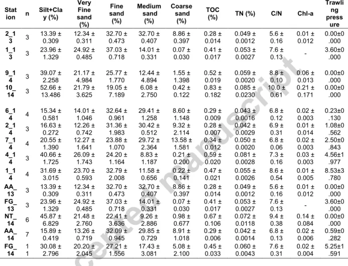
Table 2. Summary of the environmental parameters investigated (average ± SE) including: grain-size composition (%), total organic carbon (TOC, %), total nitrogen (TN, %), carbon/nitrogen (C/N), chlorophyll a content (chl-a; µg.g-1_{) and TP: trawling pressure estimates (h.km}-2_.y-1

). Stations are

ordered by the increasing trawling pressure estimates of the station in each sampling year. Trawling pressure area groups include: not trawled (NT); adjacent area to fishing ground (AA); and fishing ground (FG). Stat ion n Silt+Cla y (%) Very Fine sand (%) Fine sand (%) Medium sand (%) Coarse sand (%) TOC (%) TN (%) C/N Chl-a Trawli ng press ure 2_1 3 3 13.39 ± 0.309 12.34 ± 0.311 32.70 ± 0.473 32.70 ± 0.407 8.86 ± 0.397 0.28 ± 0.014 0.049 ± 0.0012 5.6 ± 0.16 0.01 ± 0.012 0.00±0.000 1_1 3 3 23.96 ± 1.329 24.92 ± 0.485 37.03 ± 0.718 14.01 ± 0.331 0.07 ± 0.030 0.41 ± 0.017 0.053 ± 0.0027 7.6 ± 0.13 - 3.60±0.000 9_1 4 3 39.07 ± 2.258 21.17 ± 4.984 25.77 ± 1.770 12.44 ± 4.894 1.55 ± 1.398 0.52 ± 0.019 0.059 ± 0.0020 8.8 ± 0.10 0.06 ± 0.013 0.00±0 .000 10_ 14 3 52.66 ± 13.486 21.79 ± 3.625 19.05 ± 7.189 6.08 ± 2.750 0.42 ± 0.122 0.83 ± 0.182 0.085 ± 0.0230 10.0 ± 0.61 0.21 ± 0.171 0.00±0 .000 6_1 4 4 15.34 ± 0.581 14.01 ± 1.046 32.64 ± 0.961 29.41 ± 1.258 8.60 ± 1.148 0.29 ± 0.009 0.043 ± 0.0016 6.8 ± 0.12 0.02 ± 0.003 0.23±0 .130 2_1 4 3 16.63 ± 0.272 12.26 ± 0.742 31.36 ± 1.983 30.42 ± 0.512 9.32 ± 2.114 0.28 ± 0.007 0.042 ± 0.0029 6.9 ± 0.31 0.01 ± 0.014 1.08±0 .562 7_1 4 4 20.55 ± 1.390 12.27 ± 1.641 23.88 ± 1.070 29.72 ± 2.364 13.58 ± 1.581 0.34 ± 0.012 0.050 ± 0.0020 6.8 ± 0.06 0.02 ± 0.003 2.50±0.843 4_1 4 3 40.66 ± 1.725 26.09 ± 1.743 24.20 ± 1.164 8.83 ± 1.187 0.21 ± 0.200 0.59 ± 0.020 0.081 ± 0.0028 7.3 ± 0.16 0.03 ± 0.003 4.56±1.977 1_1 4 4 31.69 ± 3.015 23.70 ± 0.593 32.79 ± 2.008 11.58 ± 0.656 0.22 ± 0.141 0.47 ± 0.021 0.055 ± 0.0026 8.6 ± 0.54 0.01 ± 0.005 8.53±3.780 AA_ 13 3 13.39 ± 0.309 12.34 ± 0.311 32.70 ± 0.473 32.70 ± 0.407 8.86 ± 0.397 0.28 ± 0.014 0.049 ± 0.0012 5.6 ± 0.16 0.01 ± 0.012 0.00±0.000 FG_ 13 3 23.96 ± 1.329 24.92 ± 0.485 37.03 ± 0.718 14.01 ± 0.331 0.07 ± 0.030 0.41 ± 0.017 0.053 ± 0.0027 7.6 ± 0.13 - 3.60±0 .000 NT_ 14 6 45.87 ± 6.829 21.48 ± 2.760 22.41 ± 3.636 9.26 ± 2.886 0.98 ± 0.677 0.67 ± 0.106 0.072 ± 0.0118 9.4 ± 0.38 0.14 ± 0.084 0.00±0.000 AA_ 14 7 15.89 ± 0.419 13.26 ± 0.719 32.09 ± 0.945 29.85 ± 0.729 8.91 ± 1.018 0.29 ± 0.006 0.042 ± 0.0014 6.8 ± 0.13 0.02 ± 0.006 0.59±0.282 FG_ 14 1 1 30.08 ± 2.796 20.20 ± 2.045 27.21 ± 1.556 17.43 ± 3.081 5.08 ± 2.100 0.45 ± 0.033 0.060 ± 0.0043 7.6 ± 0.31 0.02 ± 0.004 5.25±1.591 3.2. Macrofaunal assemblages

A total of 4695 macrofaunal individuals were ascribed to 310 different taxa, of which 77 were singletons (24.8% of the total species richness). The most abundant phylum was the Annelida (59.9% of the total abundance; 95 species), while Arthropoda was the most species-rich (24.5% of the total abundance; 147 species). Mollusca showed an intermediate relative importance in terms of abundance and number of species (10.1% of total abundance; 48 species). The remaining phyla were less represented both in terms of abundance and number of species, namely: Echinodermata (2.1%; 9 species); Cnidaria

(1.0%; 5 species); Sipuncula (2.0%; 1 species); Nemertea (0.3%; 3 species); Platyhelminthes (<1%; 1 species) and Cephalorhyncha (Class Priapulida; <1%; 1 species).

3.2.1. Multivariate analyses

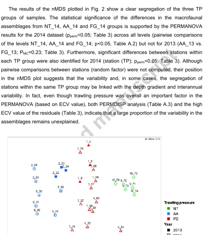
The results of the nMDS plotted in Fig. 2 show a clear segregation of the three TP groups of samples. The statistical significance of the differences in the macrofaunal assemblages from NT_14, AA_14 and FG_14 groups is supported by the PERMANOVA results for the 2014 dataset (pperm<0.05; Table 3) across all levels (pairwise comparisons of the levels NT_14, AA_14 and FG_14; p<0.05, Table A.2) but not for 2013 (AA_13 vs. FG_13; PMC=0.23; Table 3). Furthermore, significant differences between stations within each TP group were also identified for 2014 (station (TP); pperm<0.05; Table 3). Although pairwise comparisons between stations (random factor) were not computed, their position in the nMDS plot suggests that the variability and, in some cases, the segregation of stations within the same TP group may be linked with the depth gradient and interannual variability. In fact, even though trawling pressure was overall an important factor in the PERMANOVA (based on ECV value), both PERMDISP analysis (Table A.3) and the high ECV value of the residuals (Table 3), indicate that a large proportion of the variability in the assemblages remains unexplained.

Figure 2. nMDS plot for comparison of macrofauna assemblages subjected to varying trawling

(AA); and fishing ground (FG). Closed symbols: 2013 samples; open symbols: 2014 samples. Numbers above each symbol correspond to the replicate codes (station and deployment number).

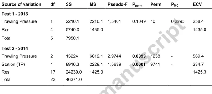
Table 3. Results of the PERMANOVA main tests. Test 1: 1-factor design (TP: trawling pressure)

applied 2013 samples; Test 2: 2-factor design (TP: trawling pressure and station (TP)) applied to the 2014 dataset. Trawling pressure levels include: not trawled (NT); adjacent area to the fishing ground (AA); and fishing ground (FG). Significant values are in bold; ECV: estimated component of variation.

Source of variation df SS MS Pseudo-F Pperm Perm PMC ECV

Test 1 - 2013 Trawling Pressure 1 2210.1 2210.1 1.5401 0.1049 10 0.2295 258.4 Res 4 5740.0 1435.0 1435.0 Total 5 7950.1 Test 2 - 2014 Trawling Pressure 2 13224 6612.1 2.9744 0.0099 1258 - 569.4 Station (TP) 4 8916.3 2229.1 1.5639 0.0001 9741 - 234.7 Res 17 24230.0 1425.3 1425.3 Total 23 46371.0

Species contributions to the differences between TP groups were examined through SIMPER analyses (Tables A.4 and A.5). Pairwise dissimilarities in community composition in 2014 ranged between 62.9 and 72.6% (AA_14 vs. FG_14 and NT_14 and AA_14, respectively). In 2013, the dissimilarity among groups was slightly lower (58.1% for AA_13 vs. FG_13). These values resulted mainly from numerous species with low contributions to the total dissimilarity (e.g. species with individual contributions > 1.5% only accounted for 12.7-15.6% of the total dissimilarity between groups; Tables A.4 and A.5). This arises from the overall low abundance of the species and high evenness of the assemblages. In fact, the highest contributions to the similarity within groups and/or dissimilarity between groups are due to fluctuations in the abundance of common species, mostly surface deposit feeding polychaetes (e.g. Aricidae, Cirratulidae, Ampharetidae, Spionidae), shared across groups (Table A.5).

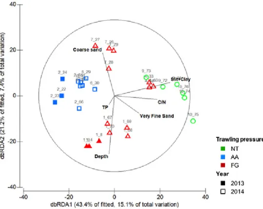
To further explore the observed variability in the macrofauna assemblages, the measured environmental parameters and biological dataset were modelled through the DISTLM routine (marginal tests) and illustrated in the dbRDA plot (Fig. 3). Nine out of the eleven examined environmental variables contributed significantly to the variation in macrofaunal composition (Table A.6). Furthermore, the variables that best contributed to

the construction of the fitted model (adjusted R2_{= 0.17866), included, by order of} importance, silt+clay content (12.3%), water depth (7.0%), C/N ratio (4.8%), trawling pressure (TP; 4.2%), coarse sand (3.5%) and very fine sand contents (3.2%), accounting for 35.0% of the total variability. The dbRDA plot, further confirms the heterogeneity within FG group encompassing stations with more variable grain size composition and a greater depth range. Although the contribution of trawling pressure for the fitted model is low, the interpretation of this result is complex because of the possible interactions with other examined variables (e.g., grain size, TOC).

Figure 3. Distance-based redundancy (dbRDA) plot illustrating the relation of the macrofaunal

assemblages and the fitted environmental variables. Fitted environmental variables (as vectors) included: water depth, fine sand (%), medium sand (%), trawling pressure (TP), and Carbon/Nitrogen ratio (C/N). Trawling pressure groups include: not trawled (NT); adjacent area to the fishing ground (AA); and fishing ground (FG). Closed symbols: 2013 samples; Open symbols: 2014 samples. Numbers above each symbol correspond to the replicate codes (station and deployment number).

3.2.2. Biomass, abundance and biodiversity

The average macrofaunal biomass (wwt, mg per 0.1 m2) varied greatly across the stations investigated (395.9–1495.5 mg per 0.1 m2). Despite the higher average biomass

recorded in NT stations (1077.8±458.71 mg per 0.1 m2_{), no significant differences were} detected between TP groups either in 2013 (U-test=3.0; p=0.700) or 2014 (K=3.485; p=1.146) (Fig. 4A,B). Because the mean individual biomass (MIB) of most organisms was much smaller than 1 mg (71.2–85.2%; Fig. 4C,D), differences in the total biomasses were determined by the presence of weightier individuals (mostly with MIB >>100 mg). For instance, in st. 10_14 (NT) biomass was mostly accounted for by one anthozoan preying on zooplankton (Ceriantharia sp1, 1372.2 mg, 38.0% of the total biomass) and five individuals of the suspension feeder Amphiura borealis (786.9 mg, 21.8%). Weightier individuals were overall absent from AA areas but were also observed in FG stations (Fig. 4C,D): a single specimen (1408.0 mg) of a polychaete belonging to the family Acoetidae, preying on macrofauna, accounted for 64.3% of the total biomass at st. 4_14 and one

Figure 4. Macrofaunal total biomass (average ± SE) per station (A) and trawling pressure group from each year (B), and matching results for the body size spectra (C, D, respectively). Each size spectrum represents the relative contributions of different Mean Individual Biomass (MIB; mg) groups to the total abundance. Trawling pressure groups include: not trawled (NT); adjacent area to the fishing ground (AA); and fishing ground (FG).

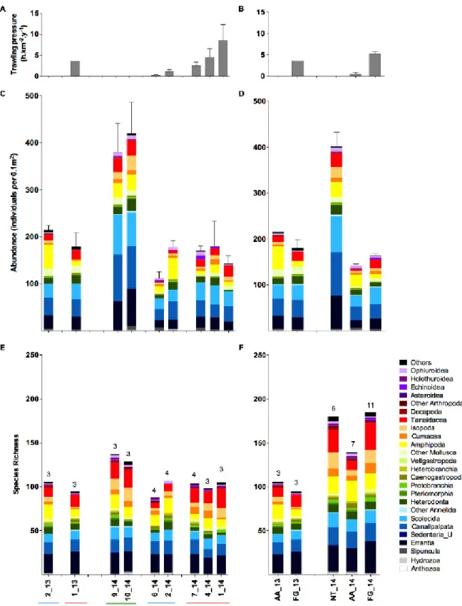
The highest macrofaunal abundances were consistently observed at NT stations (401.4±41.17 ind per 0.1 m2; Fig. 5; Table 4). In fact, abundances at NT stations were 1.8 to 3.7 times higher and significantly differed from those in either AA or FG stations in 2014 (K=12.94; p<0.05; with p<0.05 in Dunn’s post hoc test for NT_14 vs. AA_14 and NT_14 vs. FG_14), while AA and FG abundances did not significantly differ either in 2014 (Dunn’s post hoc test) or in 2013 (U=2.00; p=0.400). The same pattern was observed for the average species richness per sample with significantly higher values in NT stations in 2014 (Sav: 74.5±3.9; Table 4; K=12.13; p<0.05; with p≤0.05 in Dunn’s post hoc tests for NT_14 vs. AA_14 and NT_14 vs. FG_14) and no significant differences between AA and FG in 2013 (U=3.00; p=0.700). As for the average number of trophic guilds per sample, the higher value at NT stations (TGav: 16.0±0.45) was only significantly different from HT in 2014 (K=10.36; p<0.05; with p<0.05 in Dunn’s post hoc test for NT_14 vs. FG_14 and no significant differences in 2013: U=0.00; p=0.100). Note that the higher number of pooled species for FG_14 stations shown in Fig. 5F may be partly explained by the higher number of replicates (11) taken in this TP group. Noteworthy, biodiversity indices across all stations were characterised by a relatively high taxonomic diversity and evenness (S: 88– 137; H’: 3.88–3.99; J’: 0.804–0.876; ES(50): 29.6–32.1; ES(100): 44.3–50.3), as well as trophic diversity and evenness (TG: 15–20; H’: 2.00–2.30; J’: 0.704–0.797; ETG(50): 10.8– 12.6; ETG(100): 12.7–14.8; Table 4).

Figure 5. Overview of macrofauna abundance (average ± SE) and species richness patterns in

relation to trawling pressure. (A) Trawling pressure (TP in h.km-2_.y-1_{) per station and (B) trawling}

pressure group in each year, and matching results for to macrofaunal abundance ((C) and (D), respectively) and pooled species richness ((E) and (F), respectively). Trawling pressure groups include: not trawled (NT); adjacent area to the fishing ground (AA); and fishing ground (FG). The number of pooled replicates in each case is indicated above the bars.

Biodiversity partitioning of the 2014 assemblages in terms of species richness (Fig. 6B) estimates a large component of β-diversity (β-diversity: 78.6% vs α-diversity: 21.4%) with the largest percentage explained by differences between TP groups (β3: 39.6%) and then decreasing towards smaller special scales (β2: 20.1%; β1: 18.9%). This reflects the overall high percentage of singletons and rare (infrequent) species, but also the occurrence of distinctive species in NT and AA stations. In terms of the other indices, ES(50) and H’ (Fig. 6B), the largest biodiversity component is estimated for α-diversity (>80%) because of the little variation in community structure across all spatial scales (e.g. all assemblages, either at replicate, station or TP level, showed low dominance). Nevertheless, differences between TP groups (β3) always accounted for about one third of the total β-diversity. Similar patterns were observed in 2013 (Fig. 6A), but with higher values estimated for α-diversity (53.3, 94.1 and 85.5% for S, ES(50) and H’, respectively) which demonstrates the relevance of NT stations (not sampled in 2013) to the overall β-diversity in the region. On the other hand NT stations had much lower contribution in the differences of trophic diversity partition in 2013 and 2014 (Fig. 6C,D). The highest contribution was from the α-diversity (TG: 70.4, 70.7%; ETG(50): 86.9, 88.4%; H’: 93.9, 94.5%, for 2014 and 2013, respectively) because most trophic guilds were represented at the replicate level. Also the difference in α-diversity contribution for TG was closer to the contributions for ETG(50) and H’ because the limited number of trophic guilds (much lower than the possible number of taxa).

Figure 6. Taxonomic and trophic biodiversity partitioning for (A, C) 2013 (left) and (B, D) 2014 (right). S: number of species; H’: Shannon-Wiener diversity (log-based); ES(50): Hurlbert's expected

number of species per 50 individuals; TG: number of trophic guilds; ETG(50): Hurlbert´s expected

number of trophic guilds per 50 individuals; α: α-diversity of the sampled level - deployments; β1: β-diversity between deployments (within station); β2: β-diversity between the different stations (within areas); β3: β-diversity between trawling pressure area groups.

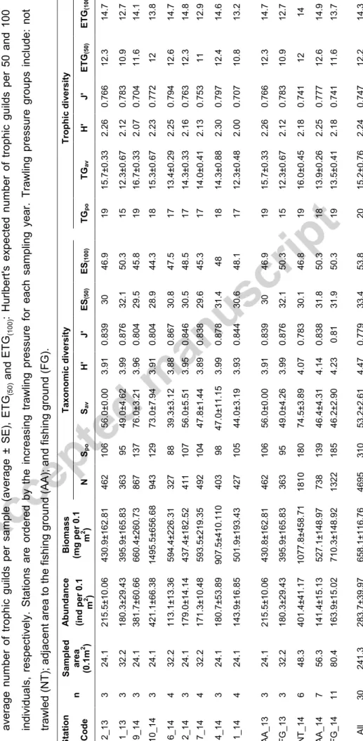
2 2 Tab le 4 . Overvie w of th e m ac rofa una l abu nda nce ( averag e ± S E ), bi o mass ( avera ge ±SE ) an d bi odi versi ty (taxono mi c and trop hic ) res ul ts fo r eac h st ati on, traw ling pre ss ur e are a gro ups per year , and st udy reg io n (All ). n: tota l numbe r of rep lica tes ; N: tota l numbe r of sp ec imens ; Spo: pooled sp ec ie s ric hnes s; S av averag e sp ec ie s ric hness per sa mple (averag e ± S E ); H’: S han non -Wi ene r di versi ty in dex (ln -bas ed) ; J’ : Pi el ou evenne ss; E S(5 0) a n d E S(1 00 ) : Hurl ber t's expec ted numbe r of sp ec ies per 50 and 100 in di vidua ls , res pec tivel y; T Gpo : poo le d num ber of trop hi c gui lds; T Ga v : averag e nu mber of tro phi c gui ld s per sa mple (averag e ± S E ), ET G(5 0) a n d ETG (1 00 ) : Hurl ber t's expec ted n umber of tr oph ic gui ld s per 50 and 100 in di vidua ls , res pec tivel y. Stati ons are ord ere d by the in cr eas in g trawl ing pre ss ure for eac h sam pl in g year . Trawl in g pre ss ure groups in cl ude : not trawl ed (NT); a dj ac ent ar ea to th e fishi ng gro und (AA); an d fi sh in g g rou nd (FG) . n Sa mpled area (0.1 m 2 ) A b un dance Biomas s (mg p er 0.1 m 2 ) Tax on omic d iv e rsit y Trop hi c di v ersity Code (in d per 0.1 m 2 ) N Sp o Sa v H ' J ' E S(50 ) E S(10 0 ) T Gp o T Ga v H ' J ' ETG (50 ) ETG (10 0 ) 2_ 1 3 3 24 .1 21 5.5 ±10.06 43 0.9 ±162 .81 46 2 10 6 56 .0± 0.0 0 3.9 1 0.8 39 30 46 .9 19 15 .7± 0.3 3 2.2 6 0.7 66 12 .3 14 .7 1_ 1 3 3 32 .2 18 0.3 ±29.43 39 5.9 ±165 .83 36 3 95 49 .0± 4.6 2 3.9 9 0.8 76 32 .1 50 .3 15 12 .3± 0.6 7 2.1 2 0.7 83 10 .9 12 .7 9_ 1 4 3 24 .1 38 1.7 ±60.66 66 0.4 ±260 .73 86 7 13 7 76 .0± 3.2 1 3.9 6 0.8 04 29 .5 45 .8 19 16 .7± 0.3 3 2.0 7 0.7 04 11 .6 14 .1 10 _ 14 3 24 .1 42 1.1 ±66.38 14 9 5.5 ±65 6.6 8 94 3 12 9 73 .0± 7.9 4 3.9 1 0.8 04 28 .9 44 .3 18 15 .3± 0.6 7 2.2 3 0.7 72 12 13 .8 6_ 1 4 4 32 .2 11 3.1 ±13.36 59 4.4 ±226 .31 32 7 88 39 .3± 3.1 2 3.8 8 0.8 67 30 .8 47 .5 17 13 .4± 0.2 9 2.2 5 0.7 94 12 .6 14 .7 2_ 1 4 3 24 .1 17 9.0 ±14.14 43 7.4 ±182 .52 41 1 10 7 56 .0± 5.5 1 3.9 5 0.8 46 30 .5 48 .5 17 14 .3± 0.3 3 2.1 6 0.7 63 12 .3 14 .8 7_ 1 4 4 32 .2 17 1.3 ±10.48 59 3.5 ±219 .35 49 2 10 4 47 .8± 1.4 4 3.8 9 0.8 38 29 .6 45 .3 17 14 .0± 0.4 1 2.1 3 0.7 53 11 12 .9 4_ 1 4 3 24 .1 18 0.7 ±53.89 90 7.5 ±410 .11 0 40 3 98 47 .0± 11 .1 5 3.9 9 0.8 78 31 .4 48 18 14 .3± 0.8 8 2.3 0 0.7 97 12 .4 14 .6 1_ 1 4 4 24 .1 14 3.9 ±16.85 50 1.9 ±193 .43 42 7 10 5 44 .0± 3.1 9 3.9 3 0.8 44 30 .6 48 .1 17 12 .3± 0.4 8 2.00 0.7 07 10 .8 13 .2 A A _1 3 3 24 .1 21 5.5 ±10.06 43 0.8 ±162 .81 46 2 10 6 56 .0± 0.0 0 3.9 1 0.8 39 30 46 .9 19 15 .7± 0.3 3 2.2 6 0.7 66 12 .3 14 .7 F G _1 3 3 32 .2 18 0.3 ±29.43 39 5.9 ±165 .83 36 3 95 49 .0± 4.2 6 3.9 9 0.8 76 32 .1 50 .3 15 12 .3± 0.6 7 2.1 2 0.7 83 10 .9 12 .7 NT _1 4 6 48 .3 40 1.4 ±41.17 10 7 7.8 ±45 8.7 1 18 1 0 18 0 74 .5± 3.8 9 4.0 7 0.7 83 30 .1 46 .8 19 16 .0± 0.4 5 2.1 8 0.7 41 12 14 A A _1 4 7 56 .3 14 1.4 ±15.13 52 7.1 ±148 .97 73 8 13 9 46 .4± 4.3 1 4.1 4 0.8 38 31 .8 50 .3 18 13 .9± 0.2 6 2.2 5 0.7 77 12 .6 14 .9 F G _1 4 11 80 .4 16 3.9 ±15.02 71 0.3 ±148 .92 13 2 2 18 5 46 .2± 2.9 0 4.2 3 0.8 1 31 .9 50 .3 19 13 .5± 0.4 1 2.1 8 0.7 41 11 .6 13 .7 All 30 24 1.3 28 3.7 ±39.97 65 8.1 ±116 .76 46 9 5 31 0 53 .2± 2.6 1 4.4 7 0.7 79 33 .4 53 .8 20 15 .2± 0.7 6 2.2 4 0.7 47 12 .2 14 .3

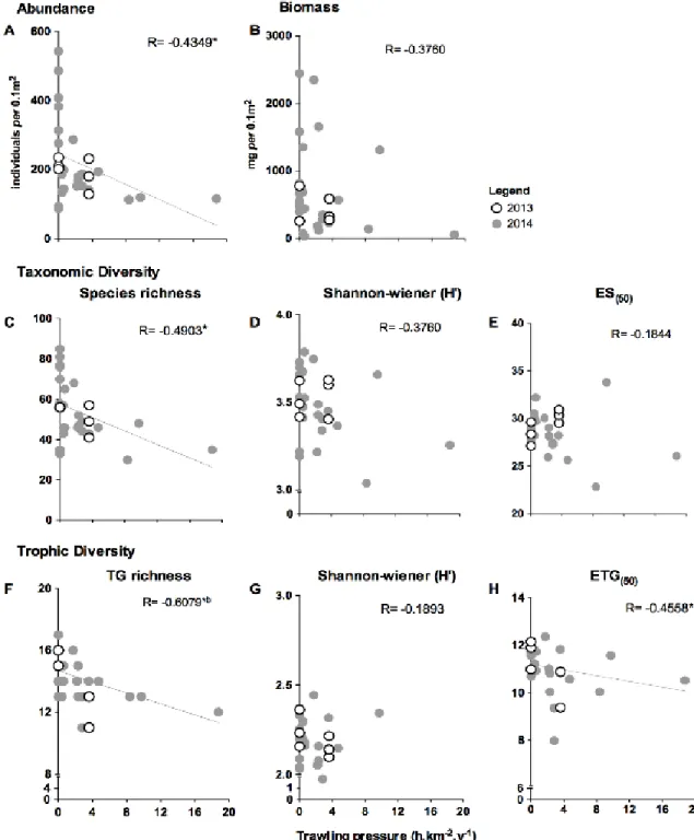
A significant negative correlation (Fig. 7), after Bonferroni correction, was detected between trawling pressure and trophic guild richness (R=-0.6079; p=0.0016); macrofaunal total abundance, species richness, and ETG(50) also showed significant correlations, but only before Bonferroni correction (R=-0.4349; p=0.0337; R=-0.4903; p=0.0150; R=-0.4558, p=0.0252, respectively). Although not statistically significant (mainly because of the high dispersion of values at 0 h.km-2.y-1), negative trends were also observed between trawling pressure and all the other estimated biodiversity indices and total biomass. Note that these values concern only the 2014 samples; the correlations were not estimated for 2013 because of the small number of samples and narrower range of trawling pressure values (Fig. 7).

Figure 7. Trawling pressure relationship with macrofauna standing stocks (i.e. (A) abundance and (B) biomass) and taxonomic and trophic diversity. Taxonomic diversity indices include: (C) species richness, (D) Shannon-Wiener taxonomic diversity, (E) Hulbert’s expected number of taxa per 50 individuals; and trophic diversity indices include: (F) number of trophic guilds; (G) Shannon-Wiener trophic diversity, (H) Hurlbert´s expected number of trophic guilds per 50 individuals. *Indicates significant correlation for 2014 samples; b_{indicates a significant correlation after Bonferroni}

3.2.3. Core assemblage composition in relation to trawling pressure

The core assemblage (Fig. 8) in NT stations was composed by a higher number of taxa (both at species level and major groups), and feeding guilds than the ones from AA and FG stations sampled in the same year (2014). In total, NT_14 core assemblage was represented by 45 different species (13 major taxa and 14 trophic guilds) grouped in 24 different combinations of major taxa and feeding guilds (Fig. 8A, Fig. A.2). These values contrast with the core assemblage of FG_14 stations composed by only 26 species (10 major taxa and 11 trophic guilds) grouped in 16 different combinations (Fig. 8C), while AA_14 showed intermediate values (31 species, 11 major taxa, 13 trophic guilds and 21 different combinations; Fig. 8B).

Overall, surface and sub-surface deposit feeders (mostly polychaetes) were the most well-represented trophic guilds in all assemblages. Additionally, both NT_14 and AA_14 core assemblages showed distinctive species from a variety of trophic guilds (11 each; Fig. A.2), but FG_14 showed no distinctive species, and a lower representation of suspension feeders and predators with an absence of microbial grazers. Distinctive species in NT_14 were suspension-feeder bivalves (Kelliella sp1, Abra longicallus,

Mendicula ferruginosa), isopods preying on macrofauna (Bullowanthura sp.,

Anthuridae sp1), omnivore polychaetes (Exogoninae sp4) and oligochaetes (Oligochaeta sp1), detritivore crustaceans (Carangoliopsis spinulosa, Pseudotanais

denticulatus) and deposit feeder polychaetes (Capitellidae sp1). Distinctive species in

AA_14 included suspension-feeder bivalves (Thyasira tortuosa), crustaceans and polychaetes predators on macrofauna (Stenothoe cf. bosphorana) and on meiofauna (Lumbrineris sp4, Nannastacus cf. unguiculatus), omnivore polychaetes

(Aponuphis bilineata) and bivalves (Yoldiella philippiana), detritivore crustaceans (Pedoculina cf. garciagomezi, Araphura sp1) and deposit feeder polychaetes (Aonidella sp1, Polycirrus sp1). In fact, the core assemblage in FG_14 stations is an impoverished subset of the other core assemblages and is formed mostly by generalist feeding guilds (deposit feeders, detritivores and omnivores) and some predator species (Fig. A.2). Trophic redundancy was higher in NT_14 core assemblage and trophic vulnerability was higher in FG_14 while AA_14 showed the highest trophic over-redundancy (TR: 3.5, 2.4, 2.4 species per trophic guild; TV: 30.8, 38.5, 54.5%; TOR: 30.8, 46.2, 27.3; for NT_14, AA_14 an FG_14, respectively).

same patterns (impoverished core assemblage in FG, with higher trophic vulnerability), but are not explored in detail here due to the limited number of replicates and stations (one in AA and one in FG area, each represented by only three replicates).

Figure 8. Core assemblage species richness for each trawling pressure group in 2014: (A) not

trawled (NT_14); (B) adjacent area to the fishing ground (AA_14) and (C) fishing ground (FG_14). Each cone represents a different combination of major taxa and trophic guild and the height of the cone represents the number of species in each combination. Macrofauna trophic guilds codes were composed of: the food source (epibenthic (EP), seafloor surface (SR) and sediment subsurface (SS)); food type/size (particulate organic matter/microfauna (mic), meiofauna (mei), macrofauna (mac)); and feeding mode (omnivorous (Om), detritus (Dt) and deposit (De) feeders, grazers (Gr), predators (Pr), mixo trophs (Mx), suspension/filter feeders (Su)). U: no information.

4. Discussion

The magnitude of the effects imposed by trawling on benthic habitats depends on the interaction of numerous factors, such as frequency and intensity of trawling activities, gears used and characteristics of the target habitats and their faunal assemblages (Kaiser et al., 2002; NRC, 2002; Hiddink et al., 2017). Thus, the assessment of trawling effects on the ecosystem requires a regional perspective for understanding the impacts, as well as regionally-adapted monitoring programmes to determine the sustainability of deep-sea fisheries (Mangano et al., 2013, 2014; Eigaard et al., 2016).

The historical importance of bottom-trawl fisheries in Portugal has led to one of the largest footprint per unit of landing in Europe bellow 200m depth, particularly in the south and southwest Portuguese margin (Eigaard et al., 2016; Bueno-Pardo et al., 2017). While both national and European programmes perform relatively frequent stock assessments of economical valuable species (MAMAOT, 2012), the knowledge of fishing impact on benthic habitats and their assemblages in the continental Portuguese deep-sea areas remains poorly known (Morais et al., 2007; Fonseca et al., 2014; Ramalho et al., 2017). Moreover, the existing assessments of Good Environmental Status (GES) have a low degree of confidence and are hindered by the limited availability of adequate control areas and the lack of pristine habitats (MAMAOT, 2012). Current legislation has imposed fishing regulations improving mostly the gear selectivity by defining minimum net mesh sizes according to the target species (Campos et al., 2007). Yet, the need to reduce the actual high bottom-trawling fishing impact, and determine adequate protected areas that insure overall resilience of the ecosystems and preserve habitats of major biological interest, makes imperative further research on the trawling impacts.

In the Portuguese margin, bottom trawlers typically target several species of deep-water crustaceans, such as the Norway lobster and rose shrimp at depths between 300-500 m water depth (Campos et al., 2007; Bueno-Pardo et al., 2017). Thus, fishing grounds overlap the habitats where these species inhabit, typically found in muddy and muddy-sand habitats; since coarser sediments are more unstable and hinder the construction and maintenance of burrows and tunnels that Norway lobsters usually construct (Afonso-Dias, 1997). Habitat characteristics also change with increasing depth (e.g. finer sediments with higher organic content at deeper locations). In this context, our results have demonstrated that the variability in macrofaunal assemblages was associated with both trawling pressure and a combination of several habitat features (depth, sediment grain size, C/N values). Still, a large component of the variability remained unexplained probably due to other

natural and anthropogenic drivers not examined in this study. The study area is located between the shelf break and upper slope close to the boundary (ca. 500 m water depth) between the North Atlantic Central Water and the Mediterranean outflow water (Llave et al., 2015) and subjected to temporal variability in the oceanographic regime (e.g. winter storms, seasonal upwelling). The different sources of spatial heterogeneity and temporal variability are typically considered as determinant in shaping the infaunal assemblages (Levin et al., 2001 and references therein).

Furthermore, we may also assume that the long trawling history in the study area may have contributed to changes in the environmental setting. For instance, seabed topography showed clear differences among the study areas (NT, AA, FG), visually confirmed by ROV video observations (Ramalho et al., 2017). Besides the flattened seabed, observed the ploughing by trawl gears promotes sediment re-suspension and changes in the sediment biogeochemistry (Puig et al., 2012). Examples are trawling induced changes in surface and sub-surface organic matter concentration, grain size composition and porosity reported by Martín et al. (2014) and Oberle et al. (2016) in the Iberian Margin and the Mediterranean Sea. These authors mention that trawling induced changes may act synergistically with natural sources of disturbance stressors.

4.1. Influence of trawling disturbance on macrofauna standing stocks and

diversity

The present study identified the negative influence of trawling pressure influence on macrofauna abundance (negative trends on biomass as well), but also the decline of species richness and changes in the community structure shown by the multivariate analysis. The reduction of the epi-benthic and infaunal standing stocks (abundance and biomass) and alterations of the community composition is one of the most frequently reported indirect effects of chronic trawling disturbance in shallow areas (Kaiser et al., 2002; NRC, 2002; Thrush and Dayton, 2002; Queirós et al., 2006; Hinz et al., 2009; van Denderen et al., 2015; Hiddink et al., 2017; Sciberras et al., 2018). These changes may derive either from the direct removal or damage of the large-sized organisms or from indirect changes in the sediment biogeochemistry characteristics and from alteration of predator-prey relationships (Duplisea et al., 2001; Jennings et al., 2001a; Mangano et al., 2015, 2017; Hinz et al., 2017). Although less frequent, similar observations were also reported from some deep-sea areas (Gage et al., 2005; Clark et al., 2015). For example, in the Mediterranean at similar depth ranges of the present study, several studies found a

significant decrease of the macrofauna abundance and biomass (Smith et al., 2000; Mangano et al., 2013, 2014).

Noteworthy is that while we observed a loss of abundance of infaunal macrobenthos, mega-epibenthic abundances did not differ between the three levels of trawling pressure (Ramalho et al., 2017, possibly due to the presence of more resilient fauna, such as the robust anemone species Spirularia ind. 5, apparently tolerant to the physical disturbance, and high abundances of mobile species that are able to avoid disturbance and/or recolonise disturbed areas over short-term periods (e.g. predatory-scavenging

Plesionika sp. and the hermit crabs Paguroidea ind. 1). By contrast, infaunal

macroinvertebrates present typically lower mobility, and may take longer to recolonise newly disturbed sediments. Furthermore, flattened surface and low evidence of bioturbation by large sized burrowing species in FG areas, contrasted with the more heterogeneous AA and NT areas (Ramalho et al., 2017). Such differences in sediment properties result in loss of habitat complexity and refugia, but also likely in alterations in the water-sediment exchanges fluxes, namely oxygen and organic matter provision deeper into the sediment (Martín et al., 2014; Oberle et al., 2016), that may all contribute to the decline of infauna standing stocks in disturbed locations (e.g. up to 3 times more individuals in NT areas, compared to AA and FG).

Declines in biomass were less clear, but trawling disturbance appeared to have prompted changes in the macrofauna size structure. The biomass in FG areas was mostly defined by accidental occurrences of a few specimens of relatively large-sized and mobile fauna (e.g. Acoetidae, Aristeus sp or Natatolana sp. 1). Contrarily, the biomass in NT areas was mostly determined by the presence of common species/taxa (with relatively high MIB), including sensitive taxa to trawling, namely by tube dwelling anemones and several individuals of the brittle stars belonging to the Amphiura genera (Smith et al., 2000; Atkinson et al., 2011; Pommer et al., 2016).

Noteworthy is that despite the differences in the species-specific composition of macrofaunal assemblages from areas with different trawling pressure shown by the multivariate analysis, these differences were not detected when considering the univariate diversity indices that are primarily based on community structure (e.g. Shannon-Wiener diversity and Pielou’s evenness), as also reported by Atkinson et al. (2011). Benthic diversity in continental slope regions is characterised by high richness and evenness (Grassle and Maciolek, 1992), and under some types of disturbance (e.g. organic pollution, eutrophication) the loss of intolerant or vulnerable species often relieves competition and is accompanied by increased abundance and dominance of opportunistic

species that take advantage from the high resource availability (Mangano et al., 2015). Bottom-trawling disturbance is predominantly physical (reworking and resuspension of sediments) and our results showed that the significant decrease both in number of species and abundance in FG areas was not compensated by increased abundance of more tolerant species. Instead it resulted in impoverished assemblages although with high evenness as no compensatory abundance effect by other species occurred. Therefore, univariate biodiversity indices (e.g. Shannon-Wiener diversity) that are used frequently as a standard monitoring tool for impact assessment in marine systems may not adequately reflect these important changes in assemblages disturbed by trawling. In the context of the MSFD 2008/56/EU descriptor 1 “biological diversity is maintained” (European Comission, 2008), these indices may even incorrectly indicate the maintenance of the Good Environmental Status (GES), and should be accompanied by other indicators of community composition, ecosystem condition and functional diversity (Strong et al., 2015).

4.2. Influence of trawling disturbance on macrofauna core community and

functional diversity

Direct effects of trawling disturbance on the fauna assemblages include high mortality of both target and non-target populations; increased food availability and loss of habitat complexity (NRC, 2002). Indirect effects of trawling disturbance on the benthic component are usually much more difficult to assess, particularly in deep-sea habitats, and include typically changes in the faunal community structure, diversity and distribution (Jennings and Kaiser, 1998; NRC, 2002; Duplisea, 2002). These changes may result in alteration of the biological interactions and trophic composition, inevitably altering the food-web structure and ecosystem functioning (Jennings et al., 2001a; Jennings et al., 2001b; Kaiser et al., 2002; NRC, 2002; Hinz et al., 2017).

In the present study, we observed an overall high macrofauna structural and functional diversity (and evenness), characteristic of the environmentally heterogeneous habitats of the shelf-slope transition region (Grassle and Maciolek, 1992; Levin et al., 2001). The analysis of compositional changes in relation to increasing levels of trawling pressure was focused in the core assemblage – a subset of the whole assemblage composed by the most abundant, frequent and distinctive taxa. The less diverse core assemblages in FG areas diverged greatly from the NT areas, likely in response to differing local conditions over long periods (decades). With the absence of distinctive taxa and packing of taxa under generalist trophic guilds (deposit feeders, detritivores and omnivores), FG core

assemblage was mostly an impoverished subset of NT and AA core assemblages. Although trophic complexity was maintained in FG areas, the depleted number of taxa across most trophic guilds represents a loss of trophic redundancy, and therefore a higher trophic vulnerability (Naeem; 1998) of these disturbed assemblages.

Local extinctions of species do naturally occur as a result of environmental fluctuations (Mouillot et al., 2014) and are usually compensated by increased abundances of sympatric, trophically redundant species and/or by the recolonization from adjacent areas, allowing in time the re-establishment of the ecosystem functions (Naeem and Li, 1997; Naeem, 1998; Liu et al., 2016). The loss of functional redundancy in FG assemblages indicates one or several of the following: i) the time between successive disturbance events prevented the re-establishment of the abundance of depleted populations; ii) the time between successive disturbance events prevented recolonization from adjacent areas; iii) there were no other trophically redundant species available locally; iv) there were no other trophically redundant species available in adjacent areas. When the loss of redundancy and/or weakening of the trophic links occurs in association with a low recolonization rate, the assemblages may either take longer to re-establish, or not recover at all, ultimately leading to trophic cascading and regime shifts (Yachi and Loreau, 1999; Belgrano, 2005; Liu et al., 2016) This shows that the resilience of assemblages affected by trawling depends crucially on the frequency of disturbance and on the existence of regional undisturbed refugia that can replenish depleted populations through recolonization.

In the case of the Portuguese margin an impressive 93.6% of the total area at depths between 200 and 1000 m are trawled annually (Eigaard et al., 2016). Areas adjacent to the fishing grounds (e.g. AA) show affected assemblages and even the few existing refugia are not exempt of anthropogenic pressures (e.g. baited traps for Norway lobster are allowed in the NT area near Setúbal canyon). Also important is the natural variability in the oceanographic regime (e.g. upwelling events) (Kämpf and Chapman, 2016), and the putative increased occurrence of climatic episodic events (e.g. winter storms) (Vitorino et al., 2002; Diogo et al., 2014), in the present scenario of global change, which may act cumulatively with trawling to increase the frequency of disturbance.

5. Conclusions

The present study indicated a depletion of macro-infaunal standing stocks (mainly abundance), as well as taxonomic and trophic richness in the fishing ground and the