I Acknowledgements
I would like to express my thanks to my supervisor, Professor Cristina Galacho, as well as to my co-supervisors, Professor Patricia Moita, and Professor José Quaresma, and to Dr. Manuela de Deus and the Direção Regional de Cultura do Alentejo. I would also like to express my deepest gratitude for the technical help and the moral support provided to me by the staff of both the Laboratório HERCULES/Universidade de Évora and the Departamento de Geociências/Universidade de Évora during the course of my Masters thesis.
II Abstract
Mirobriga is a Roman site located in the municipality of Santiago do Cacém, in Setúbal, a district in the southwest of Portugal. This settlement is mentioned in the ancient literature, and the archaeological evidence suggests that the city was developed by the Romans as an urban centre around the 1st century AD. For this study, 17 mortar samples were collected from various buildings – the Western Thermae, Domus 3, Domus 4, Taberna 1, Taberna 2, the ‘Hospedaria’, the macellum, and the forum. The chemical, mineralogical, and microstructural characterisation of the samples was performed using a number of complementary techniques – stereomicroscopy, polarised light microscopy, chemical and granulometric analysis, thermogravimetric analysis (TGA), powder X-ray diffraction (XRD), and variable pressure scanning electron microscopy-energy dispersive spectrometry (SEM-EDS). The results show that the aggregates consist mainly of quartz, whereas the binder was lime-based. The sand for the aggregates was sourced locally (within a 20 km radius), whilst the limestone for the binder may have been obtained from local quarries (within a 20 km radius), or imported from further afield (possibly from São Brissos). Most of the samples have a binder to aggregate ratio of 1 : 3, and display some degree of hydraulicity. From the results, it may be said that most of the samples are similar, indicating the contemporaneity of the buildings. Nevertheless, several samples (MRBT-1E, MRBT-2E, 12E, 13BE, MRBH7-13VE, and MRBF-16E) are different, which may be attributed to their function.
Keywords: Mirobriga, Roman mortars, stereomicroscopy, polarised light microscopy, SEM-EDS, TGA, XRD, raw materials, provenance.
III Resumo
O sítio arqueológico de Mirobriga localiza-se junto à cidade de Santigo do Cacém (distrito de Setúbal) no sudoeste de Portugal. Este sítio é mencionado na literatura antiga e as evidências arqueológicas sugerem que a cidade foi desenvolvida pelos romanos, como um centro urbano, por volta do século I dC. Para este estudo, foram recolhidas 17 amostras de argamassa de vários edifícios, nomeadamente, Termas Ocidentais, Domus 3 e 4, Taberna 1 e 2, a Hospedaria, macellum e fórum. A caracterização química, mineralógica e microestrutural das amostras foi realizada por recurso a técnicas complementares – estereomicroscopia, microscopia de luz polarizada, análise química e granulométrica, análise termogravimétrica (ATG), difração de raios-X (DRX), microscopia eletrónica de varrimento com espectroscopia de raios X por dispersão de energias (MEV-EDS). Os resultados mostram que a maioria das amostras são similares, nomeadamente, no que respeita ao tipo de agregados, com predomínio de quartzo e ao tipo de ligante, cal calcítica. A areia para os agregados era de proveniência local (num raio
de 20 km) enquanto que o calcário para o ligante pode ter sido obtido em pedreiras locais (num raio de
20 km) ou transportado de mais longe (provavelmente de São Brissos). A maioria das amostras
apresenta uma razão ligante agregado de 1:3 e um grau de hidraulicidade análogo., indicando a contemporaneidade dos diferentes edifícios estudados. As diferenças observadas em algumas amostras (MRBT-1E, MRBT-2E, MRBH7-12E, MRBH7-13BE, MRBH7-13VE, and MRBF-16E) podem ser atribuídas à função desempenhada pelas mesmas.
Palavras-chave: Mirobriga, argamassas romanas, esteromicroscopia, microscopia de luz polarizada, MEV-EDS, ATG, DRX, matérias primas, proveniências.
IV Index
1. Introduction 1
1.1. Historical Context 1
1.2. Mortar 6
1.3. Aims and Objectives 10
2. Methodology 11
2.1. Sampling 11
2.2. General Sample Preparation 11
2.3. Stereo Microscopy 11
2.4. Polarised Light Microscopy 12
2.5. Chemical and Granulometric Analysis 12
2.6. Thermogravimetric Analysis 13
2.7. Powder X-Ray Diffraction 14
2.8. Variable Pressure Scanning Electron Microscopy-Energy Dispersive Spectrometry 14
3. Results 16
3.1. Sampling and Preliminary Observations 16
3.2. Stereo Microscopy 20
3.3. Polarised Light Microscopy 21
3.4. Chemical and Granulometric Analysis 23
3.5. Thermogravimetric Analysis 31
3.6. Powder X-Ray Diffraction 33
3.7. Variable Pressure Scanning Electron Microscopy-Energy Dispersive Spectrometry 37
4. Discussion 43 4.1. Raw Materials 43 4.2. Provenance 46 4.3. Production Technology 50 5. Conclusion 58 5.1. General Conclusions 58
5.2. Suggestions for the Future 59
Bibliography 61
VIII List of Figures
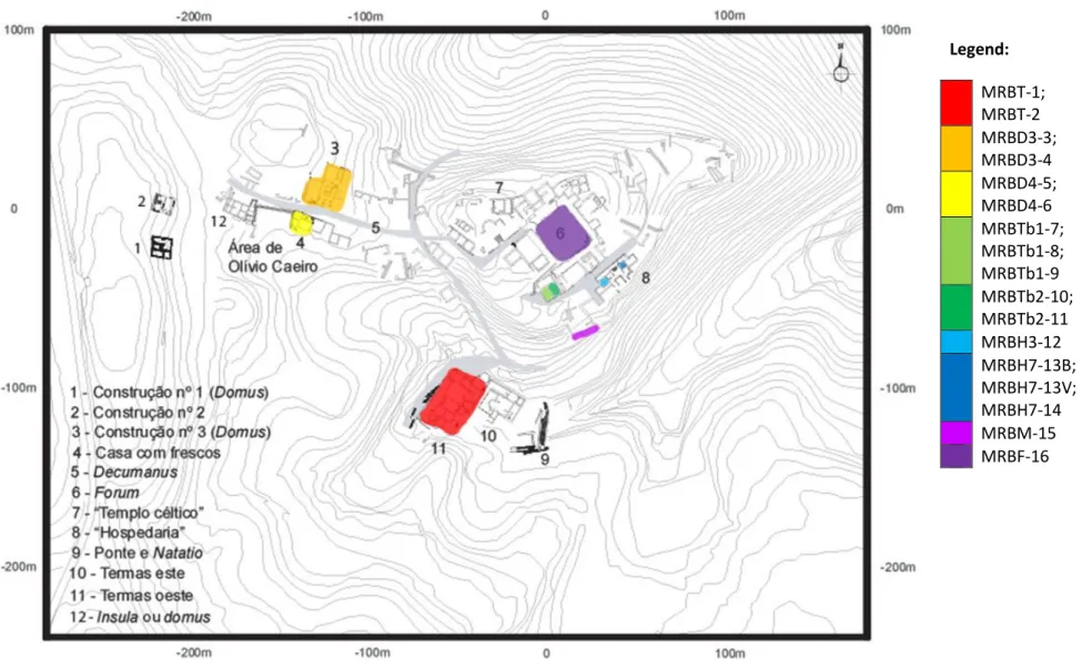
Figure 1.1. The location of Mirobriga in the Iberian Peninsula 4 Figure 1.2. The various archaeological structures at Mirobriga 4 Figure 1.3. Location of the mortar samples in the general plan of the site 5
Figure 1.4. The lime cycle 9
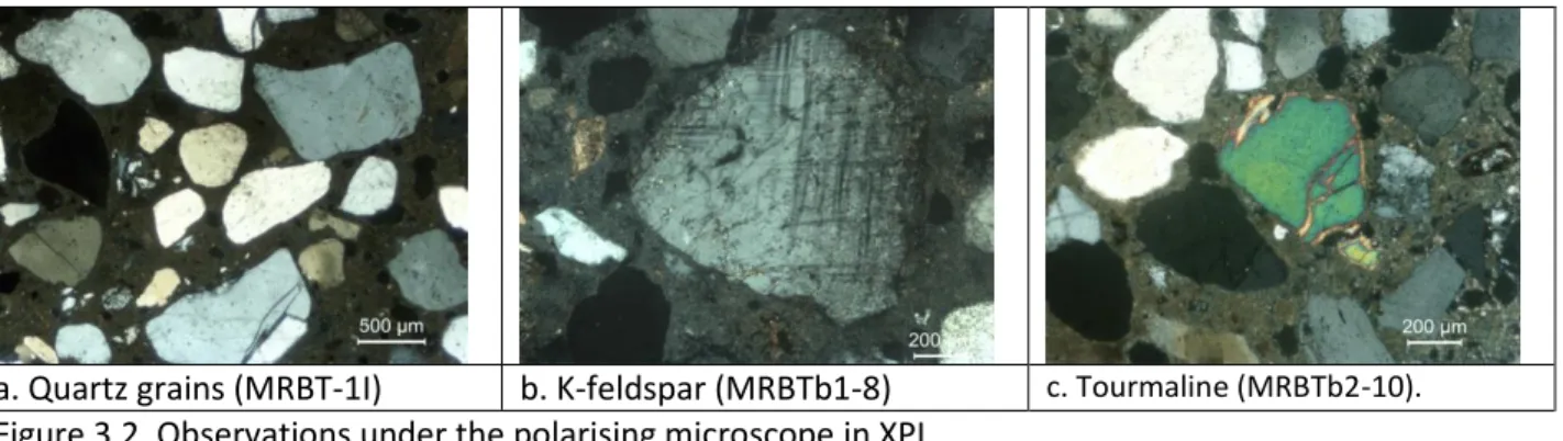
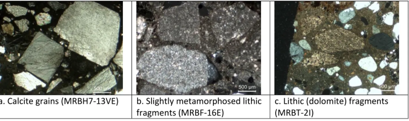
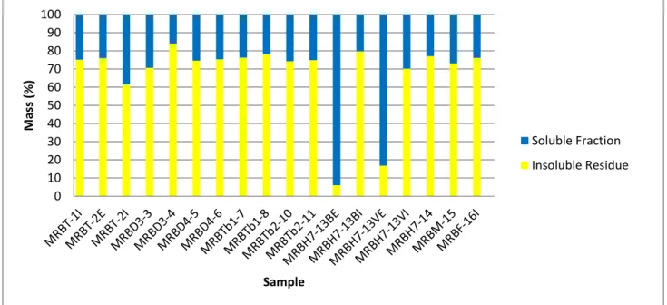
Figure 3.1. General aspects of the samples observed under the stereo microscope 20 Figure 3.2. Observations under the polarising microscope in XPL 21 Figure 3.3. Observations under the polarising microscope in XPL 22 Figure 3.4. Observations under the polarising microscope (MRBD3-4) 22 Figure 3.5. Observations under the polarising microscope (MRBD4-5) 22 Figure 3.6. The insoluble residue and soluble fraction of the samples 23 Figure 3.7. The grain size distribution of the insoluble residue,
observed under the stereo microscope (MRBTb1-7) 28
Figure 3.8. Examples of the insoluble residue observed under the stereo microscope 29
Figure 3.9. The Gravel Sand Mud Diagram 30
Figure 3.10. The TGA results of MRBT-1I, showing the thermogravimetric (TG),
and the derivative thermogravimetric (DTG) curves 31
Figure 3.11. The diffractogram of MRBD3-3 (global fraction) 33
Figure 3.12. The diffractogram of MRBD3-3 (fine fraction) 34
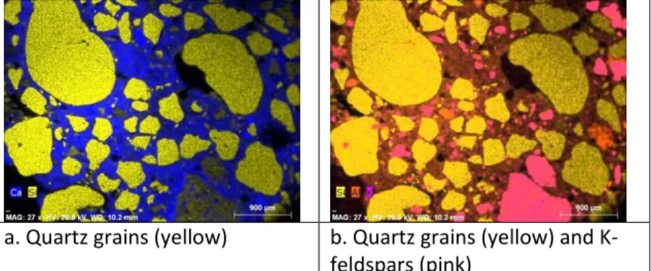
Figure 3.13. Elemental maps of MRBTb1-8 38
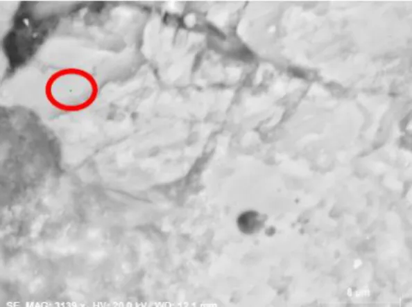
Figure 3.14. Ilmenites in MRBTb2-10 38
Figure 3.15. External and internal layers of MRBH7-13B 38
Figure 3.16. The BSE image for the point analysis performed on the binder in MRBH7-14 40 Figure 3.17. EDS spectrum of a point analysis performed on the binder in MRBH7-14 40 Figure 3.18. The BSE image for the point analysis performed on a lime lump in MRBTb1-8 41 Figure 3.19. EDS spectrum of a point analysis performed on a lime lump in MRBTb1-8 41
VIII Figure 3.20. Differences between the external and internal layers 42 Figure 3.21. Elemental maps of the transition layer in MRBT-2 42
Figure 4.1. Geological map of the area around Mirobriga 46
Figure 4.2.I. Carbon Dioxide vs Carbon Dioxide / Structurally Bound Water 54
Figure 4.2.II. Solubles vs Structurally Bound Water 55
VIII List of Tables
Table 3.1. General description of the samples 18
Table 3.2. Grain size distribution of the insoluble residue 24
Table 3.3. Description of the insoluble residue 25
Table 3.4. TGA mass change, and the carbon dioxide / structurally bound water ratio 32 Table 3.5. The semi-quantitative results of the XRD analysis (global fraction) 35 Table 3.6. The semi-quantitative results of the XRD analysis (fine fraction) 36
Table 4.1. The insoluble residue, the calcium carbonate, CaCO3,
VIII List of Annexes
Annex 2.1. Photographic Register and Observation of the Mortar Samples
under the Stereo Microscope 65
Annex 3.1. Location of the Mortar Samples in Each Structure 67
Annex 3.2. The Insoluble Residue, Soluble Fraction, and Binder to Aggregate Ratio
of the Mortar Samples 71
Annex 3.3. The Grain Size Distribution of the Insoluble Residue 72
Annex 3.4. Re-sieving of MRBT-1I (SIMAX) 75
Annex 3.5. Thermogravimetric Graphics / Thermograms 77
Annex 3.6. Powder X-Ray Diffraction (XRD) Diffractograms (Global Fraction) 80 Annex 3.7. Powder X-Ray Diffraction (XRD) Diffractograms (Fine Fraction) 84
Annex 4.1. Legend for Figure 4.1. 87
Annex 4.2. The Chemical Characteristics of Historic Mortars as
1 1. Introduction
1.1. Historical Context
The archaeological site of Chãos Salgados (more commonly known as Mirobriga) is located in the municipality of Santiago do Cacém, in Setúbal, a district in the southwest of Portugal. Situated on the western slope of the Grândola mountain range, the ruins of this Roman settlement are close to the present town of Santiago do Cacém.
Reference to Mirobriga in the ancient sources can be found in Pliny’s Natural History. In Book IV, Chapter XXII, Pliny lists ‘Mirobricenses surnamed Celtici’ (Mirobricenses qui Celtici cognominantur) as one of the tributary towns (stipendiaria) of Lusitania. Mirobriga is also mentioned in Ptolemy’s Geography, as well as in the Antonine Itinerary (Alarcão, 1976, p. 584). Be that as it may, apart from these passing references, the ancient authors are silent about Mirobriga. It may be added that although the site has been long known and identified, it was only in 1957 that Mirobriga’s identity was confirmed, in the form of inscriptions found at the site that named the settlement (Alarcão, 1967, p. 175).
Archaeology has contributed greatly to the current understanding of the site, more so than the writings of ancient authors and the epigraphic evidence. The archaeological evidence indicates that the site of Mirobriga was already occupied by the indigenous Celtici population during the Iron Age. This is apparent on the hill known as Castelo Velho, where the forum now stands. Fernando de Almeida speculated that this was where the pre-Roman settlement was situated, and was proven to be right by Tavares da Silva and Joaquina Soares, who studied the unstratified ceramics from the site (Biers et al., 1983, p. 38). Additionally, it was in this area that a “proto-Roman temple of the Celtic type”, believed to have belonged to the Late / Second Iron Age, i.e. the 4th century BC, was discovered in 1982 (Biers et al., 1983, p. 40; Slane et al., 1984, pp. 55-56). In the following year, an earlier temple, dated to the Early / First Iron Age, i.e. the 8th / 9th century BC was discovered beneath the 4th century temple (though separated by a gap, i.e. “a layer of dark earth filled with charcoal, pebble-sized schist, feldspar, quartz and small rounded pink limestones), suggesting that a settlement was already in existence during this period (Slane et al., 1984, pp. 54-56).
In the stratigraphic layer designated as the final phase of the Iron Age “Celtic Temple”, i.e. around 100 BC, Roman pottery appears for the first time, a sign that contact between the indigenous Celtic population and the Romans had been established during that time (Slane et al., 1984, p. 58). The “Roman urban development program” (Slane et al., 1984, p. 58) is reckoned to have occurred in the 1st century AD, during the reign of either Claudius or Nero, as evidenced by the “Pottery excavated from
2 beneath the foundations for paving slabs in the south corner of the forum and from beneath street paving slabs in front of the South Building” (Biers et al., 1983, p. 36). This fits the general trend that occurred in the Iberian Peninsula. The Roman provinces of Hispania Citerior and Ulterior were created in 197 BC, though it was only from the reign of Augustus onwards, i.e. the end of the 1st century BC and the beginning of the 1st century AD, that the adoption of Roman architecture can be seen in the archaeological evidence (Keay, 1995, cited in Revell, 2013, p. 386).
The settlement continued to develop during the Roman period, with new structures added or existing ones enlarged over time. As an example, the excavation of the thermae, which consists of the East Baths and West Baths, indicated that the two structures were built at different times. Pottery form the former provides a terminus post quem of the Flavian period (i.e. the second half of the 1st century AD) for its construction, whilst the building of the latter has been dated to the 2nd century AD. Mirobriga was abandoned several centuries later. Different dates, however, have been proposed regarding the abandonment of the site. The Luso-American team, for instance, point to the coins and pottery lying on the floor of one of the excavated houses as potential markers for the abandonment of the area during the 3rd / 4th century AD (Slane et al., 1985, p. 35). On the other hand, the excavation of three structures in residential area by Filomena Barata has led to the proposition that the site was abandoned during the middle of the 5th century AD (Quaresma, 1999b, cited in Quaresma, 2010, p. 350), whilst a piece of Phocaean red slip (Hayes form 3) in the abandonment layer of ‘Domus 3’ may be an indication that the site continued to be occupied up until the first half of the 6th century AD (Quaresma, 2010, p. 351).
The first modern description of Mirobriga was made during the 16th century by a Portuguese Dominican friar from Évora, André de Resende (Quaresma, 2012, p. 25). It was, however, only during the 19th century that the site was first excavated, under the direction of Frei Manuel do Cenáculo, an Archbishop of Évora (Quaresma, 2012, p. 25). The excavation of the site continued in the following century, under the direction of various archaeologists. Of note are the campaigns of Fernando de Almeida (between 1959 and 1979), during which the first monograph of the site was produced (Quaresma, 2012, p. 25; Soren & Soren, 1996, p. 76), and those of the Luso-American team during the 1980s. The latter was a collaboration between the University of Missouri-Columbia, the University of Évora, and the Southern Regional Archaeological Services of the Portuguese Institute of Cultural Heritage (Serviços Regionais de Arqueologia do Sul do Instituto Português do Património Cultural), which is noteworthy for being the first systematic investigation of the site (Quaresma, 2012, pp. 12, 25).
3 Whilst Mirobriga continued to be excavated during the 1990s, it was also during this time that its development into a tourist destination commenced. During this decade, management of the site was taken over by the Portuguese Institute of Architectural Heritage (Instituto Português do Património Arquitectónico), the lands surrounding the site were acquired, and the construction of a Reception and Interpretation Centre (Centro de Acolhimento e Interpretação) was approved (Direção-Geral do Património Cultural, Ministério da Cultura, 2011).
The excavation of Mirobriga is ongoing, and the latest project, ‘TabMir. Tabernae of Mirobriga, Chãos Salgados, Santiago do Cacém: A Study-Case on Roman and Late Antique Economy in Lusitania’ (As tabernae de Mirobriga, Chãos Salgados, Santiago do Cacém: um estudo de caso da economia romana e tardo-antiga na Lusitania), which is under the direction of José Carlos Quaresma, runs from 2016 to 2019 (J. C. Quaresma, pers. comm., 19 May 2018).
The excavations at Mirobriga over the decades have brought a variety of structures to light. The public structures, such as the forum and thermae, no doubt received the most attention due to their prominence. Nevertheless, a number of domestic structures, including several domus, and the ‘Hospedaria’ (which in fact is another domus) (J. C. Quaresma, pers. comm., 24 May 2018), have been investigated. Moreover, the commercial structures of the site are currently being studied, as part of the TabMir project. A taberna was excavated during the 2017 season, whilst a second one, as well as part of the macellum, were the focus of the 2018 season (J. C. Quaresma, pers. comm., 23 April 2018).
4 Figure 1.1. The location of Mirobriga in the Iberian Peninsula (taken from Quaresma, 2010, p. 348).
a. The Western Thermae b. Taberna 1 (left) and 2 (right) c. Domus 4
d. Domus 3 e. The macellum (cryptoporticus?) f. The forum (temple podium) Figure 1.2. The various archaeological structures at Mirobriga.
5 Legend: MRBT-1; MRBT-2 MRBD3-3; MRBD3-4 MRBD4-5; MRBD4-6 MRBTb1-7; MRBTb1-8; MRBTb1-9 MRBTb2-10; MRBTb2-11 MRBH3-12 MRBH7-13B; MRBH7-13V; MRBH7-14 MRBM-15 MRBF-16
6 1.2. Mortar
Mortar is a building material that has been widely used in various parts of the world throughout history. Due to its workability, this material has been employed for a range of purposes in the construction of buildings. Amongst other things, mortar is used to fill the gaps between bricks or stones, thereby joining them, as a render to cover the external surface of walls, and as plaster for the painting of frescoes. In general, mortar is composed of three elements – an aggregate, a binder, and water, which are combined to form a paste (Borelli, 1999, p. 3; Schnabel, 2008, p. 1).
The aggregate forms the bulk of any mortar, volumetrically speaking, and its main function is to minimise the shrinkage that may occur in the mortar paste as it sets (Schnabel, 2008, p. 1). In most instances, the aggregate is an inert material, such as sand or crushed rocks, though in some cases, chemically reactive materials, including crushed bricks or ceramics, may be used. The most regularly used aggregate in mortars is natural sand, normally in one of its two most common forms, i.e. quartz or carbonate. Through the observation of the size and shape of the sand grains, as well as the identification of trace constituents, much information about the source of the aggregate may be obtained (Schnabel, 2008, p. 2).
The binder is the material that holds the aggregate together, and may be divided into two main types – non-hydraulic and hydraulic binders. The former solidifies through dehydration (the loss of water) and carbonation (the absorption of carbon dioxide), whilst the latter uses up water during the process of solidification. Non-hydraulic binders used in the past include clay, gypsum, and lime, whilst hydraulic lime and Portland cement are some examples of hydraulic binders (Borelli, 1999, pp. 4-9; Schnabel, 2008, p. 2).
Apart from the aggregate and binder, some mortars may also contain additives and admixtures. A wide range of materials fall in this category, and includes not only inorganic materials (e.g. iron filings and crushed ceramics), but also organic ones (e.g. blood and egg whites) (Schnabel, 2008, p. 3; Sickels, 1982, cited in Schnabel, 2008, p. 3). The addition of such substances serves to modify the properties of the mortar, either aesthetically (e.g. to give colour to the mortar), or physically (e.g. to improve the strength of the mortar) (Borelli, 1999, p. 4; Schnabel, 2008, p. 3).
Roman mortar was lime-based, and the ancient Greeks have been widely credited with the initiation of its large-scale use in Europe during the Classical period (Davey, 1961, cited in Hughes & Válek, 2003, p. 5). This technology was later adopted by the Romans, who greatly improved it through the invention of concrete. The importance of this new material is evident, as it was used extensively for
7 concrete constructions across much of the Roman world from the 1st century BC onwards (Wright, 2005, p. 176).
Like all mortars, Roman lime-based mortar consisted of an aggregate, a binder (in this case lime), and water. One of the most important sources of information for the aggregate and binder used for the production of Roman mortar is Vitruvius’ On Architecture. This information may be found in Book II of his multi-volume work. It may be added that some information on this subject can also be found in Pliny’s Natural History, specifically in Book XXXVI.
Sand was commonly used as an aggregate by the Romans. In both Vitruvius’ On Architecture (Book II, Chapter IV) and Pliny’s Natural History (Book XXXVI, Chapter LIV), three different types of sand are distinguished – pit sand, river sand, and sea sand. Vitruvius goes on to discuss the advantages and disadvantages of each variety of sand, and provides simple instructions to determine whether a sand is suitable for use as an aggregate.
With the regards to thebinder, both Vitruvius (On Architecture, Book II, Chapter V, 1) and Pliny (Natural History, Book XXXVI, Chapter LIII) agree that the best lime is obtained from the burning of white limestone. Both authors also distinguish two types of stone – hard and soft, for the production of lime. The former is better suited for structural parts, whilst the latter for plasters. Additionally, the burning of lime is mentioned in both works, and a detailed explanation of the ‘science’ behind this process is provided by Vitruvius (On Architecture, Book II, Chapter V, 2):
“The reason why lime makes a solid structure on being combined with water and sand seems to be this: that rocks, like all other bodies, are composed of the four elements. Those which contain a larger proportion of air, are soft; of water, are tough from the moisture; of earth, hard; and of fire, more brittle. Therefore, if limestone, without being burned, is merely pounded up small and then mixed with sand and so put into the work, the mass does not solidify nor can it hold together. But if the stone is first thrown into the kiln, it loses its former property of solidity by exposure to the great heat of the fire, and so with its strength burnt out and exhausted it is left with its pores open and empty. Hence, the moisture and air in the body of the stone being burned out and set free, and only a residuum of heat being left lying in it, if the stone is then immersed in water, the moisture, before the water can feel the influence of the fire, makes its way into the open pores; then the stone begins to get hot, and finally, after it cools off, the heat is rejected from the body of the lime.”
8 This process is known today as the lime cycle, and is explained through chemistry as follows:
1. When calcium carbonate (CaCO3), e.g. limestone, is burnt in a kiln at high temperatures. i.e. between 900 and 1000 °C, calcium oxide (CaO), known as quicklime or burnt lime, is produced, and carbon dioxide (CO2) is released. This process is known as calcination.
CaCO3 (s)
→ CaO (s) +
CO2(g)
(Eq. 1)
2. Water (H2O) is added to hydrate the quicklime in a process known as slaking, thus forming calcium hydroxide [Ca(OH)2], which is referred to as slaked or hydrated lime. As an exothermic reaction, heat is released. If just enough water is added during the slaking process, the resultant slaked lime will be a in a dry powder form. If excess water in added, however, the final product will be in a paste form known as lime putty.
CaO (s) + H2O (l) Ca(OH)2 (s) + heat (Eq. 2)
3. As slaked lime is turned into mortar (by adding the aggregate, and additional water if necessary), applied onto a structure, and left to dry, it loses water, and absorbs carbon dioxide from the surrounding atmosphere. As a result of this, the slaked lime returns to its original form, i.e. calcium carbonate, causing the mortar to harden.
Ca(OH)2 (aq) + CO2 (g) CaCO3 (s) + H2O (l) (Eq. 3) Another piece of important information provided by the ancient authors about Roman mortar is the ratio between the binder and the aggregate. In On Architecture, Book II, Chapter V, 1, Vitruvius states that the ratio of binder depends on the type of sand. For pit sand, the ratio of binder to aggregate is given as 1:3, whilst for river and sea sand, 1:2. Pliny (Natural History, Book XXXVI, Chapter LIV), on the other hand, provides a different recipe. For pit sand, a 1:4 binder to aggregate ratio is provided, whilst for river and sea sand, 1:3. Both writers agree, however, that the quality of mortar made with river or sea sand may be improved by adding powdered baked bricks or ceramics to the mixture.
9 Figure 1.4. The lime cycle, taken and adapted from Tŷ-Mawr Lime Ltd
10 1.3. Aims and Objectives
The aims of this thesis were three-fold:
1. To identify and characterise the raw materials (the aggregate, binder, and additives) that were used for the production of the mortars.
2. To determine the provenance of the raw materials.
3. To study the technology employed for the production of the mortars.
A number of complementary techniques were used to analyse the samples. With these techniques, the chemical, mineralogical, and microstructural characterisation of the mortar could be achieved.
Additionally, by combining the results of these analyses with the geological survey of the region around Mirobriga, and with the writings of ancient Roman authors, the provenance of the raw materials, as well as the production technique of the mortars could be determined.
Moreover, comparisons between the mortars were made according to their function, and the type of structures they were taken from.
11 2. Methodology
The methodology for the analysis of the mortars in this study is as follows: 2.1. Sampling
A total of 17 mortar samples were collected from the site. Some samples (MRBT-1, MRBT-2, MRBH3-12, MRBH7-13B, MRBH7-13V, and MRBF-16) have stratigraphic layers, and hence divided into external and internal layers (marked by an ‘E’ and an ‘I’ respectively at the end of the sample’s name). The samples were taken from eight different buildings (see Annex 2.1. and 2.2.), which may be divided according to their function, i.e. domestic, commercial, or public. Archaeologists were present to aid the sample collection process.
As a general rule, mortars that could be easily dislodged were preferred, as this minimised the damage inflicted on the aesthetics of the structure. When necessary, however, a hammer and chisel was used to procure the mortar sample. In addition, several samples were obtained from the depot, where they were collected and stored during previous excavations. In certain areas, namely the thermae, where restoration work had been carried out in the past, precaution was taken not to collect the restoration material, i.e. cement. After being photographed, the samples were placed in individual transparent plastic bags, and labelled.
2.2. General Sample Preparation
The samples were photographed with a Nikon COOLPIX S2500 digital camera (see Annex 2.3.), and a preliminary visual assessment was made. The samples were dried by leaving them in an oven overnight at 50 °C. After the samples cooled down, they were cleaned using brushes and a chisel. Traces of dirt, soil, and biological colonisation were removed. The samples were observed under a Leica M205 C stereo microscope (Leica Camera AG, Wetzlar, Germany), and the images were acquired with a Leica DFC290 HD digital camera (Leica Camera AG, Wetzlar, Germany) (see Annex 2.3.).
The specific sample preparation for each technique will be discussed in the sections that follow. 2.3. Stereo Microscopy
Stereo microscopy was used to provide a preliminary assessment of the samples in terms of consistency, morphology and dimension of the aggregates, inclusions (eg. ceramic fragments), and the presence of stratigraphic layers.
12 A Leica M205 C stereo microscope (Leica Camera AG, Wetzlar, Germany) was used to observe the samples, and the images were acquired with a Leica DFC290 HD digital camera (Leica Camera AG, Wetzlar, Germany).
2.4. Polarised Light Microscopy
Polarised light microscopy was used for the visual identification of the aggregates within the samples, as well as their grain size and texture.
In the samples where stratigraphy was present (MRBT-1, MRBT-2, MRBH3-12, MRBH7-13B, MRBH7-13V, and MRBF-16), the pieces were removed by cutting them with the Discoplan-TS (Struers, Cleveland, Ohio, USA), so as to preserve the stratigraphic layers. The rest of the samples were removed with the aid of a rubber mallet and a chisel. The samples were then embedded in epoxy resin (EpoFix Resin and EpoFix Hardener, Struers, Cleveland, Ohio, USA), in accordance with the manufacturer’s instructions. The embedding was done at room temperature and pressure. After the resin hardened, the surface of each sample was polished by hand with P # 280 SiC paper, and then with P # 1000 SiC paste. The glass slides were also mechanically polished with the P # 400 SiC paste on a millstone. Once the polishing of the samples and the slides were completed, resin (EpoThin resin and EpoThin hardener, 2.0 : 0.9) was used to mount the samples onto the slides, after which they were left overnight under pressure. The samples were cut using the diamond blade of a Discoplan-TS (Struers, Cleveland, Ohio, USA), and grinded with the same machine. The samples were then polished by hand using P # 1000 SiC paste until a thinness of 0.03 mm was reached. The final polishing was done with P # 4000 SiC paper, and the samples were coated with a layer of lacquer for protection.
The finished thin sections were observed with a Leica DM2500 P polarising microscope (Leica Camera AG, Wetzlar, Germany), under both plane polarised light (PPL) and cross polarised light (XPL), and the images were acquired with a Leica MC170 HD digital camera (Leica Camera AG, Wetzlar, Germany).
2.5. Chemical and Granulometric Analysis
Chemical analysis was used to determine the ratio between the soluble fraction and the insoluble residue of the samples, whilst granulometric analysis was used mainly to quantify the size distribution of the grains in the insoluble residue. The latter also allowed the composition and morphology of the insoluble residue to be identified.
13 Approximately 20 g of material was removed from the main samples. MRBTb1-9 and MRBH3-12 were not analysed, as there was not enough material. Additionally, for MRBT-2, MRBH7-13B, and MRBH7-13V, each stratigraphic layer was prepared and analysed separately. On the other hand, the analysis was only performed on the internal layers of MRBT-1 and MRBF-16.
The samples were subjected to acid attack (10 g) with hydrochloric acid (HCl, concentration of 1:3 v/v %, 120 mL), heated to boiling temperature for 10 minutes, filtered in vacuum, and washed with distilled water. By this means, the soluble fraction and insoluble residue were separated. The insoluble residues were left to dry overnight (in an oven at around 50 °C), and weighed the following day. The procedure was performed in duplicate, and the average values of the results from each sample were recorded.
Granulometric analysis was performed by sieving the insoluble residue with a stainless steel sieve (ASTM E11, diameter of 100 mm x 40 mm, with the following mesh sizes: 4, 2, 1, 0.500, 0.250, 0.125, and 0.063 mm). The different fractions of the insoluble residue were weighed, and observed under a Leica M205 C stereo microscope (Leica Camera AG, Wetzlar, Germany), after which images were acquired with a Leica DFC290 HD digital camera (Leica Camera AG, Wetzlar, Germany). The average values of the results obtained from each sample were recorded.
2.6. Thermogravimetric Analysis
Thermogravimetric Analysis (TGA) was used primarily to quantify the amount of binder with a carbonate composition. The first derivative of the TG curve (the DTG curve) shows the rate of change of the sample’s mass during the analysis, and allowed the decomposition temperature of certain compounds in the samples to be determined more accurately. By combining the results of this analysis with those obtained from the chemical analysis, the aggregate: carbonate: solubles ratio of the samples could be calculated.The global fraction was used for this analysis.
The samples were first grounded into a fine powder. With the exception of MRBH3-12 (both external and internal layers), which was grounded manually with an agate mortar and pestle, the rest of the samples were grounded with a ball mill, Planetary Ball Mill PM 100 (Retsch GmbH, Haan, Germany), at 500 rpm for a duration of 10 minutes. It may be added that for MRBT-2, MRBH3-12, MRBH7-13B, MRBH7-13V, and MRBF-16, each stratigraphic layer was prepared and analysed separately, whilst the analysis was only performed on the internal layer of MRBT-1.
14 The powdered samples were analysed in a simultaneous thermal analyser, STA 449 F3 Jupiter (NETZSCH-Gerätebau GmbH, Selb, Germany), under inert atmosphere (nitrogen – 70 ml/min.), with a uniform heating velocity of 10°C/min. from 40 to 1000 °C.
2.7. Powder X-Ray Diffraction
Powder X-Ray Diffraction (XRD) was used to determine the mineralogical composition of the samples by identifying their crystalline phases. The global and the fine fractions (which contains a higher concentration of the binder, i.e. particles < 0.063 mm in size) of the samples were used for this analysis.
For both analyses, it was necessary for the samples to be grounded into a fine powder. For the global fraction, this was done with a ball mill, Planetary Ball Mill PM 100 (Retsch GmbH, Haan, Germany), at 500 rpm for a duration of 10 minutes. MRBH3-12 (both external and internal layers) was the exception, as it was grounded manually with an agate mortar and pestle. For MRBT-2, MRBH3-12, MRBH7-13B, MRBH-13V, and MRBF-16, each stratigraphic layer was prepared and analysed separately, whilst for MRBT-1, only the internal layer was analysed. As for the fine fraction, the samples were first disaggregated using a rubber mallet, and then passed through a stainless steel sieve with a mesh size of 0.063 mm (ASTM E11, diameter of 100 mm x 40 mm). XRD analysis of the fine fraction was not performed on MRBD4-5, MRBTb1-9, and MRBH3-12, as well as MRBT-1E, MRBH7-13BE, MRBH7-13VE, and MRBF-16E.
The diffractograms were produced using an X-ray diffractometer, Bruker AXS-D8 Advance (Bruker Corp, Billerica, Mass. USA), with Cu-Kα radiation (λ = 0.1540598 nm), under the following conditions: scanning between 3° and 75° (2θ), scanning velocity of 0.05° 2θ/s, accelerating voltage of 40 kV, and current intensity of 30 mA.
2.8. Variable Pressure Scanning Electron Microscopy-Energy Dispersive Spectrometry
Scanning Electron Microscopy (SEM) was utilised for imaging purposes, which allowed the morphology of the aggregates to be assessed. To a lesser extent, a preliminary elemental analysis (based on brightness) was undertaken. The process made use of the back-scattered electrons (BSE) produced by the samples. Energy Dispersive Spectroscopy (EDS), on the other hand, utilised the X-ray emissions from the samples for elemental analysis, elemental mapping, and punctual analyses.
A small piece of each sample was selected for this technique. A rubber mallet and a chisel were used to remove these pieces. In the samples where stratigraphy was present (MRBT-1, MRBT-2, MRBH3-12, MRBH7-13B, MRBH7-13V, and MRBF-16), the pieces were removed by cutting them with the
15 Discoplan-TS (Struers, Cleveland, Ohio, USA), so as to preserve the stratigraphic layers. Next, the samples were observed under a Leica M205 C stereo microscope (Leica Camera AG, Wetzlar, Germany), and images were acquired with a Leica DFC290 HD digital camera (Leica Camera AG, Wetzlar, Germany). Epoxy resin (EpoFix Resin and EpoFix Hardener), prepared in accordance with the manufacturer’s instructions, was used to embed the samples. The embedding was done at room temperature and pressure. After the resin hardened, the surface of each sample was polished by hand. Silicon carbide (SiC) paste of different grit sizes, i.e. P # 400, P # 800, and P # 1000 (from coarse to fine) was used. The final polishing of the samples was done on SiC paper (P # 2400 and P # 4000).
A Hitachi S-3700N SEM (Hitachi High Technologies, Berlin, Germany) coupled with a Bruker XFlash 5010 SDD detector (Bruker Corp, Billerica, Mass. USA) was used for the sample analysis. The analysis samples were performed under low vacuum, i.e. 40 Pa, with a current of 20 kV. The spectra were plotted on an energy scale of 0-20 keV, with a spectral resolution of 129 eV at Mn Kα.
16 3. Results
3.1. Sampling and Preliminary Observations
A general description of each sample is presented in Table 3.1, which includes the following aspects: the structure and location where each sample was collected from, the historical period, the function of the mortar, their colour, and inclusions seen in them.
The samples were collected from public, commercial, and domestic buildings. From the public buildings, two samples (MRBT-1 and MRBT-2) (Annex 3.1., Figure 1) were collected from the thermae, whilst a sample was collected from the forum (MRBF-16) (Annex 3.1., Figure 5). From the commercials buildings, five samples were taken from two tabernae, Taberna 1 (7, 8, and MRBTb1-9) (Annex 3.1., Figure 4), and Taberna 2 (MRBTb2-10, and MRBTb2-11) (Annex 3.1., Figure 4), whereas from the macellum, a sample (MRBM-15) (Annex 3.1., Figure 4) was collected. The rest of the samples were collected from domestic buildings, i.e. the domus, and the ‘Hospedaria’. For the former, two samples each were collected from Domus 3 (MRBD3-3 and MRBD3-4) (Annex 3.1., Figure 2), and Domus 4 (MRBD4-5 and MRBD4-6) (Annex 3.1., Figure 3). As for the latter, a sample was collected from Room 3 of the ‘hospedaria’ (MRBH3-12) (Annex 3.1., Figure 4), whilst three samples were taken from Room 7 of the same structure (MRBH7-13B, MRBH7-13V, and MRBH-14) (Annex 3.1., Figure 4). Most of the samples were collected from walls, though several of them were taken from other parts of the buildings. MRBD3-4, and MRBD4-5 were taken from stairs, the former being attached to Domus 3, whilst the latter coming from the street outside Domus 4. MRBTb2-11 was collected at the entrance of Taberna 2, whereas MRBM-15 was taken from what is believed to be the cryptoporticusof the macellum.
All the structures have been dated to the Roman period, specifically between the 1st and 2nd centuries AD. As the samples may be said to be contemporaneous, it would neither be possible nor necessary to divide the samples according to historical periods.
The samples may be classified according to their function. The majority of them have been identified as filling mortars, though several of them, namely MRBT-1, MRBTb1-9, and MRBH7-14, have been designated as rendering mortars. In certain samples (MRBT-1, MRBT-2, MRBH3-12, MRBH7-13B, and MRBH7-13V, and MRBF-16), stratigraphic layers were identified, and these layers served different functions. MRBT-2I served as a filling mortar, MRBT-2E functioned as a render. MRBH3-12, MRBH7-13B, and MRBH7-13V were taken from frescoes, and, in addition to the chromatic layer, contain two stratigraphic layers that may be considered to be mortars. The internal layer of these three samples may either be the “very rough rendering coat” or the “layers of sand mortar”, as described by Vitruvius in his
17 treatment of stucco work (On Architecture, Book VII, Chapter III, 5). As for the outer layer of these samples, these are likely to be Vitruvius’ “layers of marble powder” (On Architecture, Book VII, Chapter III, 6). Although the rendering coat / sand mortar, and marble powder layer were also visible in MRBT-1 and MRBF-16, it may be noted that it is unclear whether these samples once had chromatic layers on them.
In terms of colour, the samples are quite uniform, as most of them are beige in colour. The exceptions are MRBT-1E, MRBT-2E, MRBH3-12E, MRBH7-13BE, and MRBH7-13VE, MRBF-16E. These samples are white in colour, with the exception of MRBT-2E, which has a red colour.
As for inclusions, lime lumps were visible in almost all of the samples, whilst numerous samples contained ceramic fragments. The latter is especially evident in MRBT-2E, and the red colour of this layer is due to the addition of powdered bricks / ceramics. In addition, relatively large lithic fragments (as aggregates) were observed in certain samples, for instance, MRBT-2I and MRBD3-3.
18 Table 3.1. General description of the samples.
Sample Structure Location Period Function Colour Inclusions Notes
MRBT-1 Western Thermae
Frigidarium; south wall; internal; from the upper
part of the wall
Roman
E: Layer of
'powdered marble' E: White -
Two layers of mortar I: Rendering /
'sand mortar' for stucco
I: Beige Lime lumps
MRBT-2 Western Thermae
Frigidarium;north wall; internal; between marble skirting and wall
Roman E: Rendering E: Red
E: Lime lumps,
ceramic fragments Heterogeneous stratigraphy; external layer very fragile I: Filling I: Beige I: Lime lumps, stones
MRBD3-3 Domus 3 North wall; external Roman Filling Beige Lime lumps, stones
MRBD3-4 Domus 3 Stairs; external Roman Filling Beige Lime lumps
MRBD4-5 Domus 4 Stairs from the street Roman Filling Beige Lime lumps MRBD4-6 Domus 4 North wall; internal Roman Filling Beige Lime lumps MRBTb1-7 Taberna 1 South wall; external;
from the top of the wall Roman Filling (?) Beige
Lime lumps, ceramic fragments MRBTb1-8 Taberna 1
East wall; internal, between Tb1 and Tb2; from the top of the wall
Roman Filling (?) Beige Lime lumps, ceramic fragments
MRBTb1-9 Taberna 1
North wall; internal, from the vertical face of
the wall
Roman Render (?) Beige Lime lumps
MRBTb2-10 Taberna 2
East wall; external;
adjacent to the street Roman Filling Beige Lime lumps
MRBTb2-11 Taberna 2 Entrance Roman Filling Beige
Lime lumps, ceramic fragments
MRBH3-12
'Hospedaria', Room 3
North wall; internal; wall
with paintings Roman
E: Layer of 'powdered marble'
E: Orange,
white - Heterogeneous stratigraphy;
internal layer fragile; chromatic layer and two
layers of mortar I: Rendering /
'sand mortar' for stucco
19 Table 3.1. General description of the samples (cont.).
MRBH7-13B
'Hospedaria',
Room 7 Northeast wall; internal Roman
E: Layer of
'powdered marble' E: White - From the depot;
homogenous stratigraphy, chromatic layer, two layers
of mortar I: Rendering /
'sand mortar' for stucco
I: Beige I: Lime lumps
MRBH7-13V
'Hospedaria',
Room 7 Northeast wall; internal Roman
E: Layer of 'powdered marble'
E: Red,
white - From the depot;
homogenous stratigraphy, chromatic layer, two layers
of mortar I: Rendering /
'sand mortar' for stucco
I: Beige I: Lime lumps, stones
MRBH7-14
'Hospedaria',
Room 7 South wall; internal Roman Rendering Beige Lime lumps
MRBM-15 Macellum
Back of structure, cryptoporticus (?);
internal (?)
Roman Filling Beige Lime lumps Macellum yet to be
excavated
MRBF-16 Forum Podium of the temple Roman
E: Layer of
'powdered marble' E: White -
Two layers of mortar I: Rendering /
'sand mortar' for stucco
20 3.2. Stereo Microscopy
The results of stereo microscopy suggest that, as a whole, there is little difference, in terms of composition, between the samples. Within each individual sample, however, the composition may be said to be heterogeneous. The use of stereo microscopy also allowed the stratigraphic layers of MRBT-1 and MRBF-16 to be verified.
For the majority of the samples, the aggregate consists mainly of hyaline and milky quartz (some of the latter possibly being feldspars). The quartz grains may be described as uniform, and its roundness ranging from ‘subangular’ to ‘well-rounded’ (Figure 3.1.a.). Black minerals (later identified as ilmenite), and lime lumps (associated with the binder) (Figure 3.1.b.) were also visible in the samples.
Both layers of MRBT-2 are noticeably different from the rest of the samples. MRBT-2E is distinct due to the red colour of its binder, and the presence of ceramic fragments (Figure 3.1.e.) of various colours, i.e. red, grey, and black, as aggregates, whilst the use of a higher quantity of relatively large lithic fragments (as aggregates) (Figure 3.1.d.) were observed in MRBT-2I. Additionally, a transitional layer (Figure 3.1.f.) was observed between the two layers of this sample. MRBT-1E, MRBH3-12E, MRBH7-13BE, MRBH7-13VE, and MRBF-16E are also clearly different, due to the presence of ‘angular’ / euhedric calcite grains (Figure 3.1.c., see yellow arrow) in them.
a. Hyaline quartz and milky quartz / feldspar (MRBD3-4)
b. A lime lump (MRBTb1-9) c. Chromatic layer and calcite crystals (MRBH3-12)
d. A lithic (dolomite) fragment (MRBT-2I)
e. A ceramic fragment (MRBT-2E)
f. The transition layer in MRBT-2 Figure 3.1. General aspects of the samples observed under the stereo microscope.
21 3.3. Polarised Light Microscopy
With this technique, it may be remarked that for the majority of the samples, quartz (Figure 3.2.a.) is the principal constituent of the aggregate. This mineral is present either as single grains, or as lithic fragments, i.e. quartzite, and the roundness of the grains range from ‘subangular’ to ‘well-rounded’. Feldspars (both K-feldspar and plagioclase) (Figure 3.2.b.) were also commonly found in the samples. Ilmenite was viewed under PPL, whilst tourmaline (Figure 3.2.c.) is present in many of the samples, albeit in small quantities, i.e. one or two grains.
a. Quartz grains (MRBT-1I) b. K-feldspar (MRBTb1-8) c. Tourmaline (MRBTb2-10). Figure 3.2. Observations under the polarising microscope in XPL.
In MRBT-1E, MRBH3-12E, MRBH7-13BE, MRBH7-13VE, and MRBF-16E, large calcite grains (Figure 3.3.a.) were observed. It may be added that these grains have an ‘angular’ / euhedric form. In MRBF-16E, two different types of carbonates were observed, one being the aforementioned calcite grains, whilst the other having a more rounded form, as well as a sparitic texture (Figure 3.3.b.). These are probably fragments of slightly metamorphosed limestone.
A relatively high amount of carbonates, which are possibly fragments of dolomite limestone, was also observed in MRBT-2I (Figure 3.3.c.). Due to its sparitic texture, these carbonates have been identified as lithic fragments, as opposed to crystal grains. This type of carbonate is also visible in trace amounts in some of the other samples, for example, MRBD3-3 and MRBTb2-10.
22 a. Calcite grains (MRBH7-13VE) b. Slightly metamorphosed lithic
fragments (MRBF-16E)
c. Lithic (dolomite) fragments (MRBT-2I)
Figure 3.3. Observations under the polarising microscope in XPL.
Several ‘oddities’ were also noticed in the samples. The quantity of these features may be described as ‘extremely minute’, i.e. one or two crystals / fragments in one specific sample. Of most interest are the ones seen in MRBD3-4 and in MRBD4-5. In the former, a fragment of charcoal (Figure 3.4.) was visible, whilst in the latter, a fragment of oolitic limestone (Figure 3.5.) was identified. In a study conducted by Pavía & Caro (2008), a mortar sample was found to contain “abundant, evenly distributed charcoal”, and the authors suggested that this charcoal could have been deliberately added as a pozzolan. Considering that there was only one fragment of charcoal in MRBD3-4, as opposed to being spread out evenly throughout the sample, it is unlikely that this were the case.
a. The charcoal fragment (XPL) b. The charcoal fragment (PPL) Figure 3.4. Observations under the polarising microscope (MRBD3-4).
a. The oolitic limestone (XPL) b. The oolitic limestone (PPL) Figure 3.5. Observations under the polarising microscope (MRBD4-5).
23 3.4. Chemical and Granulometric Analysis
The results of these two analytical techniques are divided into four parts – the amount of insoluble residue to soluble fraction, the granulometric fractions, the stereo microscopic observation of the insoluble residue, and the classification of the aggregate.
Figure 3.6. The insoluble residue and soluble fraction of the samples.
Figure 3.6.shows the amount of insoluble residue and soluble fraction (in percentage) of each sample, whilst the exact values of these components are provided in Annex 3.1. In MRBH7-13BE and MRBH7-13VE, the amount of insoluble residue is 5.98% and 16.76% respectively. These are the only two samples in which the amount of insoluble residue is lower than that of the soluble fraction. As carbonates were used as aggregates in these samples, they would have been dissolved during the acid attack. Therefore, the soluble fraction of these samples consists of both the aggregate and the binder. For the rest of the samples, the amount of soluble residue is higher than that of the insoluble fraction, and ranges from 61.47% in MRBT-2I to 84.08% in MRBD3-4. The insoluble residue and the soluble fraction may be equated with the aggregate and binder respectively, and hence has been used for the calculation of the binder to aggregate ratio (eg. Cardoso, 2011; Velosa et al., 2007). It may be mentioned that this calculation would not be possible for MRBH7-13BE and MRBH7-13VE, considering that the soluble fraction of these samples contain both the aggregate and the binder.
0 10 20 30 40 50 60 70 80 90 100 M ass (% ) Sample Soluble Fraction (%) Insoluble Residue (%)
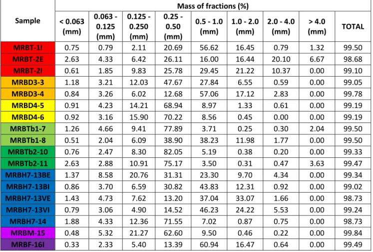
24 Table 3.2. Grain size distribution of the insoluble residue.
Sample Mass of fractions (%) < 0.063 (mm) 0.063 - 0.125 (mm) 0.125 - 0.250 (mm) 0.25 - 0.50 (mm) 0.5 - 1.0 (mm) 1.0 - 2.0 (mm) 2.0 - 4.0 (mm) > 4.0 (mm) TOTAL MRBT-1I 0.75 0.79 2.11 20.69 56.62 16.45 0.79 1.32 99.50 MRBT-2E 2.63 4.33 6.42 26.11 16.00 16.44 20.10 6.67 98.68 MRBT-2I 0.61 1.85 9.83 25.78 29.45 21.22 10.37 0.00 99.10 MRBD3-3 1.18 3.21 12.03 47.67 27.84 6.55 0.59 0.00 99.05 MRBD3-4 0.84 3.26 6.02 12.68 57.06 17.12 2.83 0.00 99.78 MRBD4-5 0.91 4.23 14.21 68.94 8.97 1.33 0.61 0.00 99.19 MRBD4-6 0.92 3.16 15.90 70.22 8.56 0.45 0.00 0.00 99.19 MRBTb1-7 1.26 4.66 9.41 77.89 3.71 0.25 0.30 2.04 99.50 MRBTb1-8 0.51 2.04 6.09 38.90 38.23 11.98 1.77 0.00 99.50 MRBTb2-10 0.76 2.47 8.30 82.05 5.19 0.38 0.20 0.00 99.33 MRBTb2-11 2.63 2.88 10.91 75.17 3.50 0.31 0.47 3.63 99.47 MRBH7-13BE 1.37 8.58 20.76 31.31 23.30 9.70 4.34 0.00 99.34 MRBH7-13BI 0.86 3.70 6.59 30.82 43.83 12.31 0.92 0.00 99.02 MRBH7-13VE 1.43 4.73 7.62 13.20 37.04 33.07 1.66 0.00 98.73 MRBH7-13VI 0.79 3.06 4.90 14.52 46.23 24.22 5.53 0.00 99.24 MRBH7-14 1.88 4.33 12.36 71.55 7.02 0.87 0.75 0.00 98.73 MRBM-15 0.48 5.32 21.27 62.60 9.50 0.46 0.22 0.00 99.84 MRBF-16I 0.33 2.33 5.40 13.39 60.94 16.47 0.64 0.00 99.49
Table 3.2. shows the grain size distribution of the insoluble residue for each sample. The graphic presentation of the data may be found in Annex 3.2. In terms of modality, all but one sample may be classified as unimodal. The predominant fraction for these samples is either 0.25 – 0.50 mm or 0.5 – 1.0 mm, the former being a ‘fine fraction’, whilst the latter a ‘medium fraction’, according to the designation provided by Coutinho (1999, p. 31). MRBTb1-8 is the only sample that may be described as bimodal, as it has both 0.25 – 0.50 mm and 0.5 – 1.0 mm as its predominant fraction. These factors, i.e. size and volume of the granulometric fractions, have an effect on the physical-mechanical properties of the mortars produced. Experiments conducted by Grassl et al. (2010), for instance, found that the shrinkage-induced micro-cracking of mortars was influenced by the size and fractional volume of the aggregates in them.
25 Table 3.3. Description of the insoluble residue.
Sample Modality Sorting**
Predominant Fraction (mm) Predominant Mineral Other Minerals / Lithics, and Additives
Roundness of Aggregates Textural Group* Aggregate Classification*
MRBT-1I Unimodal Moderately Sorted 0.5 - 1.0 (56.62%) Quartz (hyaline, milky) Quartzite, feldspar, ilmenite, tourmaline (?), clays / micas Subangular - Well-rounded Slightly Gravelly Sand
Slightly Fine Gravelly Coarse Sand
MRBT-2E Unimodal Poorly Sorted 0.25 - 0.50 (26.11%) Quartz (hyaline, milky) Quartzite, feldspar, clays / micas, ceramic
fragments (red, yellow, grey) Subangular - Well-rounded Gravelly Sand
Very Fine Gravelly Medium Sand
MRBT-2I Unimodal Poorly Sorted 0.5 - 1.0 (29.45%) Quartz (hyaline, milky) Quartzite, feldspar, ilmenite, tourmaline (?), clays / micas Subangular - Well-rounded Gravelly Sand
Very Fine Gravelly Coarse Sand MRBD3-3 Unimodal Moderately Sorted 0.25 - 0.50 (47.67%) Quartz (hyaline, milky) Quartzite, feldspar, ilmenite, tourmaline (?), clays / micas Subangular - Well-rounded Slightly Gravelly Sand
Slightly Very Fine Gravelly Medium Sand MRBD3-4 Unimodal Moderately Sorted 0.5 - 1.0 (57.06%) Quartz (hyaline, milky) Quartzite, feldspar, clays / micas Subangular - Well-rounded Slightly Gravelly Sand
Slightly Very Fine Gravelly Coarse Sand MRBD4-5 Unimodal Moderately Well Sorted 0.25 - 0.50 (68.94%) Quartz (hyaline, milky) Quartzite, feldspar, clays / micas Subangular - Well-rounded Slightly Gravelly Sand
Slightly Very Fine Gravelly Medium Sand MRBD4-6 Unimodal Moderately Well Sorted 0.25 - 0.50 (70.22%) Quartz (hyaline, milky) Quartzite, feldspar, ilmenite, tourmaline (?), clays / micas Subangular - Well-rounded
Sand Moderately Well Sorted Medium Sand MRBTb1-7 Unimodal Moderately Well Sorted 0.25 - 0.50 (77.89%) Quartz (hyaline, milky) Quartzite, feldspar, ilmenite, tourmaline (?), clays / micas Subangular - Well-rounded Slightly Gravelly Sand
Slightly Fine Gravelly Medium Sand
26 Table 3.3. Description of the insoluble residue (cont.).
MRBTb1-8 Bimodal Moderately Sorted 0.25 - 0.50 (38.90%); 0.5 - 1.0 (38.23%) Quartz (hyaline, milky) Quartzite, feldspar, ilmenite, tourmaline (?), clays / micas Subangular - Well-rounded Slightly Gravelly Sand
Slightly Very Fine Gravelly Medium Sand MRBTb2-10 Unimodal Well Sorted 0.25 - 0.50 (82.05%) Quartz (hyaline, milky) Quartzite, feldspar, ilmenite, tourmaline (?), clays / micas Subangular - Well-rounded Slightly Gravelly Sand
Slightly Very Fine Gravelly Medium Sand MRBTb2-11 Unimodal Moderately Well Sorted 0.25 - 0.50 (75.17%) Quartz (hyaline, milky) Quartzite, feldspar, ilmenite, tourmaline (?), clays / micas Subangular - Well-rounded Slightly Gravelly Sand
Slightly Fine Gravelly Medium Sand MRBH7-13BE Unimodal Poorly Sorted 0.25 - 0.50 (31..31%) Quartz (hyaline, milky) Quartzite, feldspar, clays / micas Subangular - Well-rounded Slightly Gravelly Sand
Slightly Very Fine Gravelly Medium Sand MRBH7-13BI Unimodal Moderately Sorted 0.5 - 1.0 (43.83%) Quartz (hyaline, milky) Quartzite, feldspar, ilmenite, tourmaline (?), clays / micas Subangular - Well-rounded Slightly Gravelly Sand
Slightly Very Fine Gravelly Coarse Sand
MRBH7-13VE Unimodal Poorly Sorted 0.5 - 1.0 (37.04%) Quartz (hyaline, milky) Quartzite, feldspar, clays / micas, red-coloured powder (from
chromatic layer) Subangular - Well-rounded Slightly Gravelly Sand
Slightly Very Fine Gravelly Coarse Sand
MRBH7-13VI Unimodal Poorly Sorted 0.5 - 1.0 (46.23%) Quartz (hyaline, milky) Quartzite, feldspar, ilmenite, tourmaline (?), clays / micas Subangular - Well-rounded Gravelly Sand
Very Fine Gravelly Coarse Sand MRBH7-14 Unimodal Moderately Well Sorted 0.25 - 0.50 (71.55%) Quartz (hyaline, milky) Quartzite, feldspar, ilmenite, tourmaline (?), clays / micas Subangular - Well-rounded Slightly Gravelly Sand
Slightly Very Fine Gravelly Medium Sand MRBM-15 Unimodal Moderately Sorted 0.25 - 0.50 (62.60%) Quartz (hyaline, milky) Quartzite, feldspar, clays / micas Subangular - Well-rounded Slightly Gravelly Sand
Slightly Very Fine Gravelly Medium
27 Table 3.3. Description of the insoluble residue (cont.).
MRBF-16I Unimodal Moderately Sorted 0.5 - 1.0 (60.94%) Quartz (hyaline, milky) Quartzite, feldspar, ilmenite, tourmaline (?), clays / micas Subangular - Well-rounded Slightly Gravelly Sand
Slightly Very Fine Gravelly Coarse Sand
* According to the Folk and Ward Method, as used by GRADISTAT ** According to GRADISTAT.
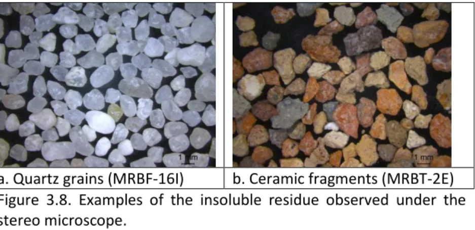
28 Table 3.3. provides a description of the insoluble residue. A summary of the observations made with the stereo microscope forms part of this table. As expected, the bulk of the insoluble residue is made up of quartz (both hyaline and milky) (Figure 3.8.a.). The roundness of these grains range from ‘subangular’ to ‘well-rounded’. It may also be noted that in certain samples, lumps of clay minerals were visible in the 0.25-0.50 mm, 0.125-0.250 mm, and 0.063-0.125 mm fractions, due to a lack of disaggregation during the sieving of the insoluble residue. A sample, MRBT-1I was re-sieved (see Annex 3.4.), and the results suggest that the values of the 0.063 – 0.125 mm and/or < 0.063 mm fractions may be higher, whilst those of the 0.25-0.50 mm and/or 0.125-0.250 mm and/or 0.063-0.125 mm fractions lower, than the values plotted on the graphs. These differences, however, are minor, and do not affect the granulometric results drastically. Nevertheless, the re-sieving shows that the clay content of the samples, as represented by the 0.063 – 0.125 mm and < 0.063 mm fractions, is higher than originally shown.
a. > 4.0 mm b. 2.0 - 4.0 mm c. 1.0 - 2.0 mm
d. 0.5 - 1.0 mm e. 0.25 - 0.50 mm f. 0.125 - 0.250 mm
Figure 3.7. The grain size distribution of the insoluble residue, observed under the stereo microscope (MRBTb1-7).
29 a. Quartz grains (MRBF-16I) b. Ceramic fragments (MRBT-2E)
Figure 3.8. Examples of the insoluble residue observed under the stereo microscope.
In addition, Table 3.3. displays some of the results, i.e. the sorting, textural group, and classification of the insoluble residue from the analysis performed using GRADISTAT, a particle size analysis software written by Simon Blott (downloaded from http://www.kpal.co.uk/gradistat.html) (Kenneth Pye Associates Ltd, 2018). It may be added that although a European standard for aggregates (European Standard EN 13139:2002 Aggregates for mortar) is available, this was not used, as it did not contain a classification of the aggregate fractions according to their size.
The results suggest that the aggregate in all the samples consists of sand, as opposed to mud or gravel, though of different textures, i.e. either ‘Sand’, ‘Slightly Gravelly Sand’ or ‘Gravelly Sand’. Moreover, the sorting of the aggregate ranges from ‘poorly sorted’ to ‘well sorted’. This sorting has an effect on the workability of the mortar (Schnabel, 2008, p. 1), and has been shown to affect the final quality of the mortar (see, for example, Arizzi and Cultrone, 2013).
30 Figure 3.9. The Gravel Sand Mud Diagram.
31 3.5. Thermogravimetric Analysis
The thermograms presented in Annex 3.5. show the results of the Thermogravimetric Analysis (TGA). The thermogravimetric (TG), as well as the derivative thermogravimetric (DTG) curves of each sample are displayed in these figures, whereas Table 3.4. shows the mass change (in percentage) of the samples. Additionally, the carbon dioxide / structurally bound water ratio is also presented in the table. The 40-120 °C, 200-600 °C, and 600-950 °C ranges corresponds to the change in mass attributed to the physically bound / absorbed water (also referred to as hygroscopic water), the structurally bound water (also referred to as chemically bound water or hydraulic water), and the decomposition of carbonates (more specifically the calcites) (resulting in the release of carbon dioxide) respectively (Bakolas et al., 1998; Moropoulou et al., 1995).
Figure 3.10. The TGA results of MRBT-1I, showing the thermogravimetric (TG), and the derivative thermogravimetric (DTG) curves.
32 Table 3.4. TGA mass change, and the carbon dioxide / structurally bound water ratio.
Sample Mass Change (%) Carbon Dioxide / Structurally Bound Water 40-120 °C 120-200 °C 200-600 °C 600-950 °C Total MRBT-1I 0.49 0.03 -0.74 -8.59 -8.81 11.61 MRBT-2E -0.58 -0.99 -2.06 -4.33 -7.96 2.10 MRBT-2I 0.21 -0.03 -0.78 -15.16 -15.76 19.44 MRBD3-3 0.20 -0.02 -0.89 -9.52 -10.23 10.70 MRBD3-4 -0.16 -0.15 -0.76 -3.52 -4.59 4.63 MRBD4-5 -0.06 -0.28 -1.41 -7.76 -9.51 6.81 MRBD4-6 -0.36 -0.24 -2.01 -13.48 -16.09 6.71 MRBTb1-7 -0.11 -0.12 -0.82 -7.57 -8.62 9.23 MRBTb1-8 -0.19 -0.27 -1.36 -7.94 -9.76 5.84 MRBTb1-9 -0.17 -0.23 -2.07 -11.73 -14.20 5.67 MRBTb2-10 -0.11 -0.08 -1.14 -7.78 -9.11 6.82 MRBTb2-11 -0.24 -0.26 -1.27 -7.88 -9.65 6.20 MRBH3-12E -0.03 -0.08 -1.69 -29.84 -31.64 17.66 MRBH3-12I -0.41 -0.31 -2.53 -8.38 -11.63 3.31 MRBH7-13BE -0.07 -0.12 -1.15 -37.99 -39.33 33.03 MRBH7-13BI -0.27 -0.20 -1.41 -6.44 -8.32 4.57 MRBH7-13VE -0.09 -0.12 -1.41 -32.32 -33.94 22.92 MRBH7-13VI 0.39 -0.12 -1.08 -9.99 -10.80 9.25 MRBH7-14 0.00 -0.07 -1.09 -7.89 -9.05 7.24 MRBM-15 -0.47 -0.37 -1.18 -4.43 -6.45 3.75 MRBF-16E -0.41 -0.38 -1.80 -26.18 -28.77 14.54 MRBF-16I -0.06 -0.15 -0.66 -7.96 -8.83 12.06
In Table 3.4., it may be remarked that mass change in the 200-600 °C range (attributed to the structurally bound water) is low in the samples, the lowest being -0.66% (MRBF-16), and the highest being -2.53% (MRBH3-12I). On the contrary, the change in mass in the 600-950 °C (attributed to the calcite decomposition, during which carbon dioxide is released) varies between the samples, ranging from -3.52% in MRBD3-4 to -37.99% in MRBH7-13BE. In most of the samples, the carbon dioxide content may be described as ‘low’, i.e. < 10.00%. The rest of the samples may either be described as having a ‘medium’ (10–20 %) or ‘high’ (> 20%) proportion of calcite. MRBT-2I, MRBD4-6, and MRBTb1-9 belong to the former, whilst MRBH3-12E, MRBH13-BE, MRBH7-13VE, and MRBF-16E belong to the latter. The
33 ‘high’ amount of calcite in the latter four samples was expected, as their aggregate consist mainly of this mineral.
With the values in the 200-600 °C and 600-950 °C ranges, i.e. the amount of structurally bound water and the carbonates, the carbon dioxide / structurally bound water ratio could be calculated. This ratio has been used as an indicator of a mortar’s level of hydraulicity (Bakolas et al., 1998; Moropoulou et al., 1995; Moropoulou et al., 2005), and will be discussed further in the following chapter.
3.6. Powder X-Ray Diffraction
Table 3.5. shows the semi-quantitative results of the Powder X-Ray Diffraction (XRD) analysis on the global fractions, whereas those of the fine fractions are presented in Table 3.6. The diffractograms of the global and fine fractions are presented in Annexes 3.6. and 3.7. respectively. The results of the XRD analyses provide an overview mineralogical composition of the samples, as well as a semi-quantitative analysis of these minerals.
Figure 3.11. The diffractogram of MRBD3-3 (global fraction). Legend: Q – quartz; C – calcite; F – K-feldspar.
34 Figure 3.12. The diffractogram of MRBD3-3 (fine fraction).
35 Table 3.5. The semi-quantitative results of the XRD analysis (global fraction).
Sample Mineral
Quartz Calcite K-Feldspar Plagioclase Micas Dolomite Aragonite
MRBT-1I ++++ + ++ + ++ - - MRBT-2E +++ + ++ + ++ - - MRBT-2I ++++ + ++ - ++ + - MRBD3-3 ++++ ++ ++ - - - - MRBD3-4 ++++ + ++ - - - + MRBD4-5 +++ + ++ - +++ - - MRBD4-6 ++++ + ++ - - - - MRBTb1-7 ++++ + ++ - ++ - - MRBTb1-8 ++++ + ++ - ++ - - MRBTb1-9 ++++ + ++ - + - - MRBTb2-10 ++++ + + - + - - MRBTb2-11 ++++ + ++ - + - - MRBH3-12E ++ ++++ + - - - - MRBH3-12I ++++ ++ + + ++ - - MRBH7-13BE + ++++ ++ + - ++ - MRBH7-13BI ++++ + ++ - + - - MRBH7-13VE ++ ++++ + - - - - MRBH7-13VI ++++ + ++ + - - - MRBH7-14 ++++ + + - - - - MRBM-15 ++++ + ++ - + - - MRBF-16E ++++ +++ + - - - - MRBF-16I ++++ + + - - - -
++++ (very high proportion / predominant mineral); +++ (high proportion); ++ (medium proportion); + (low proportion); - (undetected)
In Table 3.5, it is clear that quartz is the predominant mineral in almost all of the samples. By contrast, calcite exists either in small or medium quantities in these samples. The inverse is true for MRBH3-12E, MRBH7-13BE, and MRBH7-13VE, where calcite is the predominant mineral, as expected, whereas quartz is present either in low or medium quantities. It may be added that in the case of MRBF-16E, whilst quartz is the predominant mineral, a high amount of calcite was detected as well. Feldspars were also detected in the samples. K-feldspar was detected in all of the samples (either in small or medium proportions), whilst plagioclase was found only in several of the samples. In addition, the presence of micas was detected in several samples, whilst dolomite was observed in two samples (MRBT-2I and MRBH7-13BE). Finally, aragonite was detected in MRBD3-4.
36 Table 3.6. The semi-quantitative results of the XRD analysis (fine fraction).
Sample Mineral
Quartz Calcite Mg Calcite K-Feldspar Plagioclase Micas Clays Dolomite Ilmenite Tourmaline Aragonite Gypsum
MRBT-1I ++ ++++ ++ ++ + - - tr. - + - ? MRBT-2E +++ ++ ++ + + ++ + + tr. + - - MRBT-2I + ++++ ++ + - - ++ + tr. + - - MRBD3-3 ++ +++ ++ ++ - ++ ++ tr. tr. + - - MRBD3-4 ++ +++ ++ ++ + - ++ tr. + + ++ - MRBD4-6 ++ ++++ ++ ++ - ++ + tr. tr. + - - MRBTb1-7 ++ +++ ++ + - ++ ++ tr. - + - - MRBTb1-8 ++ ++++ ++ ++ + ++ + + - + - - MRBTb2-10 ++ +++ ++ + + ++ +++ tr. - - - - MRBTb2-11 +++ +++ ++ ++ + + + + tr. + - - MRBH7-13BI ++ +++ ++ ++ - ++ ++ + tr. + - - MRBH7-13VI ++ ++++ +++ ++ + - ++ tr. + + - - MRBH7-14 +++ +++ ++ ++ + ++ + tr. - + - - MRBM-15 +++ +++ + ++ + ++ + + tr. + - - MRBF-16I + +++ ++ ++ tr. ++ + +++ tr. + - -
++++ (very high proportion / predominant mineral); +++ (high proportion); ++ (medium proportion); + (low proportion); tr. (traces); ? (uncertain); - (undetected)