Predicting extreme equity returns with binary response models

(1)

A Work Project, presented as part of the requirements for the Award of a Master Degree in Finance from the NOVA – School of Business and Economics

Predicting Extreme Equity Returns with

Binary Response Models

Author: Julian Riedel

Student-ID: 2519

A Project carried out on the Master in Finance Program, under the

supervision of:

Afonso Eça

(2)

Abstract

In this paper a parsimonious methodology for estimating the probability of observing an extreme negative movement in monthly stock returns is proposed. It uses Extreme Value Theory to define an extreme return and exploits dynamic probit models based on (Kauppi and Saikkonen 2008) which are expected to improve the performance of the regression. The results are convincing, as the dynamic feature indeed enhances the models’ performance. Moreover, successive extreme returns are observed, confirming the fact of extremal clustering in the tails of the distribution.

(3)

List of Tables

Table I – Summary statistics ... 13

Table II – Estimation Results – Static Model ... 17

Table III – Estimation Results – Pure Dynamic Model ... 19

Table IV – Estimation Results – Pure Autoregressive Model ... 23

(5)

List of Figures

Figure 1: Historical S&P500 Prices and Log-Returns. ... 12 Figure 2: QQ-Plot of S&P500 return series against the standard normal distribution ... 14 Figure 3: Hill-Plot ... 15

(6)

1. Introduction

Explaining the returns of common stocks has a long tradition in financial literature, and bears high practical value. For instance, it is extremely relevant for institutional investors, such as pension funds or endowments, as well as for individuals: having an idea in of how a security performs, gives an investor the opportunity to invest accordingly and take advantage of the situation. Thus, gaining on its competitive edge vis-à-vis its competitors. If asset pricing theory forecasts returns positively, an investor might take on a long position in this security, meaning she will invest in that stock, while she will not invest if the predicted return is negative. This is a valid approach, as it provides the possibility to decide among different investment opportunities. She can buy and sell based on asset pricing theory, but again, this is merely a comparison among different stocks. An investor might be equally interested in having the knowledge to receive an absolute signal, more specifically: a large, sudden drop in her equity investment. These plunges usually wipe out the majority of the value created during bullish markets. Recent examples include the financial crisis 2008, and the dotcom bubble 2001. But what if an investor is able to forecast such large drops, coined as extreme returns? Clearly, she can protect herself, either by selling that investment or by hedging the position. This is on the one hand valuable for risk management purposes in financial institutions and on the other hand can give the risk-loving investor an additional investment opportunity through short-selling. Therefore, the aim of this paper is to predict extreme tail-events by the means of parsimonious, yet dynamic econometrics modelling approaches. More specifically it focusses on the left-tail of the distribution: on large, extreme losses. It follows commonly applied methodologies to define an ‘extreme return’ and anticipates those movements with binary response models. It explicitly compares different model specifications to obtain a parsimonious model to avoid overfitting. The parsimonious aspect enters through a dynamic feature which is expected to enhance the explanatory power while ensuring a simplistic model.

(7)

The rest of this paper thus proceeds as follows. Chapter two provides an overview of relevant literature on forecasting equity returns and introduces. Chapter three explains the methodology, while section four states the research hypotheses. Subsequently, chapter five introduces the data set and steps to prepare it for the research purposes. Section six provides empirical results. Chapter seven outlines potential limitations, while chapter eight concludes.

2. Literature Review

Over the last 70 years, predicting returns on equity has been an exhaustive strand of academic research. Many different explanatory variables have been identified which have shown more or less predictive power on equity returns. They can be broadly divided into the categories microeconomic and macroeconomic indicators of return predictability. The difference is, that microeconomic is directly ‘linked’ with the stock or index to be examined, thus generally measuring the price in relation to its underlying fundamentals (Lewellen 2004), while macroeconomic variables might affect the entire economy. Important research on microeconomic variables has been conducted in several papers, which ultimately conclude that aggregate dividend ratios can have sizeable power to explain equity returns (Campbell and Shiller 1988a, Campbell and Shiller 1988b, Hodrick 1992, Rozeff 1984). The dividend-yield, and its close relative the dividend-price-ratio have been subject to several studies and are assumed to have statistical power to predict equity returns, especially over a one-year horizon (Goyal and Welch 2003). Taking a closer look at accounting measures reveals that a long-term moving average of earnings-price-ratio has predictive power on future stock returns (Campbell and Shiller 1988a), as well as earnings as a variable in general (Shiller 1984). Combining those two fundamental measures leads to the dividend pay-out ratio, which has been used by Lamont (1998) to predict equity returns. He concludes that dividends use forward-looking information, while earnings incorporate current information because they are highly correlated with the business cycle. Additionally, balance sheet items can be used to forecast equity returns. The

(8)

book-to-market ratio, calculated as a firm’s book value over its current market value, has been proven to provide predictive power (Lewellen 2004, Pontiff and Schall 1998), especially in the short-run (Kothari and Shanken 1997). Nevertheless, Lewellen (2004) stresses that the forecasting ability is remarkably lower compared to the dividend-yield. The assumption behind this predictive power on equity returns is that the book value is an expectation of future cash flows (Pontiff and Schall 1998), therefore increasing returns with the book-to-market ratio. Macroeconomic variables have also been widely applied to forecast equity returns. Hjalmarsson (2010) shows that the short-term interest rate has predictive power for equity returns in developed countries, and moreover, he finds that the term spread, as the difference between short-term and long-term rate also exhibits a strong ability to forecast returns. The interpretation behind the short-term interest rate might be found in the fact that a higher rate decreases the attractiveness of equity investments vis-à-vis bond investments in terms of risk and returns, as well as in terms of discount factor. Thus a higher rate would lead to the expectation of lower equity returns. Jordan, Vivian, and Wohar (2014) confirm this studies with respect to the short-term rate for some major European economies in an out-of-sample approach. The same principle can be assumed for the long-term interest rate as it is closely related and correlated with the short-term rate. Empirically, Hall, Anderson, and Granger (1992) and Stock and Watson (1988) find that both rates exhibit a long-term relationship and cointegrate, which also makes the long-term interest rate an applicable explanatory variable.

Common for all of these studies is, that they focus on forecasting the average return of stocks. None of them explicitly examines the predictive power of those variables for the tail of the distribution, e.g. an extreme return. This is relevant for portfolio hedges, as pointed out above, because one main characteristic of equity returns is, that they exhibit so-called fat-tails. This stylized fact means that equity returns exhibit high absolute returns (negative or positive) significantly more often than expected under a Gaussian normal distribution (Mandelbrot 1963,

(9)

Fama 1965). Loosely speaking, this means, that more events are cumulated in the tails of the distribution. The underlying reason is somewhat debated among researcher, but it is generally attributed to market inefficiencies. Among others, Poterba and Summers (1988) conclude that market inefficiency is due to irrational behaviours among capital market participants, while financial news might also be an important source of market inefficiency (Bondt and Thaler 1985). Thus, assessing the likelihood of an extreme return seems to be equally relevant and has indeed applied already. Fodor et al. (2013) explicitly examine extreme returns, defined by a threshold of 3% (-2.5%) for the positive (negative) end, and find common characteristics among firms that tend to have a higher probability to experience extreme returns. They use a probit regression to estimate the likelihood of such a return. Similarly, Nyberg (2011) applies a probit model to forecast the direction of the US stock market. He uses dynamic specifications for his models, which will also be the main application of this paper. The exact specifications are based on Kauppi and Saikkonen (2008) who introduced the family of dynamic binary response models to forecast US recession by only using one explanatory variable, the term spread, defined as the difference between the long-term and short-term interest rate. This yields a parsimonious model, which nevertheless captured the occurrence of recessions very well. The additional power of the dynamic specification has subsequently been applied to better predict currency crisis and to develop an early warning system to predict them (Candelon, Dumitrescu, and Hurlin 2014). The reason for the good performance of the dynamic specification is the persistence of crises, which means that a crisis, observed today does not quickly disappear tomorrow. The same also holds for equity returns which experience autocorrelation (Lewellen 2002). Nevertheless, the findings are mixed whether there exists positive or negative (e.g. mean reversion) persistence, especially depending on the horizon under scrutiny. Pan (2010), finds that in the short-run (e.g. monthly return series) autocorrelation is negative, while in the long-run (e.g. annual) it tends to be positive. Transferred to extreme returns, this would mean an

(10)

extreme return today might decrease the probability of observing an extreme return tomorrow. However, Lo and MacKinlay (1988) and Poterba and Summers (1988) find exactly the opposite: in the short-run the autocorrelation is positive. This is more in line with the expectations for extreme returns, which would ultimately result in extremal clustering (e.g. successive extreme returns). All these empirical findings are generally consistent with the rejection of the efficient market hypothesis that asset returns follow a random walk which has been a large body of asset pricing literature (Poterba and Summers 1988).

However, returning to forecasting absolute equity returns, just choosing a cut-off value randomly is somehow arbitrarily, thus extreme values provide a useful approach. Diebold and Rudebusch (1991) point out that extreme value theory is highly relevant for modelling asset returns and risk management purposes, as estimates using the entire distribution are not very well suited to assess the likelihood of extreme events. This can be attributed to the fact that classical statistics usually focus on the mean, thus the average value of a sample population, which can be used as a consistent estimator, given a reasonably large sample, widely-known as the law of large numbers (Beirlant et al. 2006). However, describing a sample by its first two moments is valid, nevertheless a normal distribution might not always be appropriate, due to the fat-tail property of financial returns. Thus, two different approaches exist to model the tails of a return distribution: assuming a distribution with fatter-tails, or specifically assessing the tails of the distribution, which is the aim of the EVT-approach (Stoyanov et al. 2011). For the former full-modelling approach one could either opt for the Student’s t-distribution or for the stable Paretian distribution, which exhibit heavier tails than the normal distribution. The Student’s t distribution is symmetric in nature, while the stable Paretian is skewed to the left, which makes it a good fit for modelling financial returns which are often left-skewed due to loss-aversion properties of investors. However, if an investor is concerned only with the extreme adverse events, she might not be interested in modelling the entire distribution.

(11)

Therefore, the domain of extreme value theory helps to better study the characteristics of extreme events (LeBaron and Samanta 2005), or stated otherwise: focussing on the tail of the distribution. It gives an estimate of the probability of events that are located outside of the available sample range, thus one events that have not yet been observed.

3. Methodology

The methodology section first works through the domain of extreme value theory to define an extreme event and subsequently presents the different econometric models.

3.1 Defining an Extreme Return

The first natural question is how to define an extreme event, which is located in the tail of the distribution. Naturally, one could choose the cut-off value somewhat arbitrarily, such as -5%. However, this does not provide any information about extreme events in which we are interested (McNeil 1999), thus EVT can help to describe the behaviour more precisely. Heavy-tailed financial returns are depicted by a power decay in the tails, meaning that the probability of observing an extreme event is higher, compared to the normal-distribution. Loosely speaking, this implies that we observe extreme outlier more often than under Gaussian assumptions. In the remainder of this paper, it is assumed that the observed returns are in the domain of attraction of the Frechet distribution, which is characterized by a power law, as well as theoretically unbounded returns (LeBaron and Samanta 2005).1 This is suitable for financial returns as there is basically no maximum loss. Moreover, it is assumed that the asset returns are represented by a random variable, which is independent and identically distributed (iid), which is crucial for the application of extreme value theory. Mathematically, we want to estimate the tail index parameter α which incorporates information on the decay (e.g. the mass in the tail) of the sample and ultimately defines the length of the tail (e.g. what is considered as an extreme

1_{For an extensive, mathematical review the interested reader might consult: (LeBaron and Samanta 2005, Beirlant}

(12)

observation). The starting point is to calculate monthly returns, denoted x as the natural logarithm of this month’s price over last month’s price. Subsequently, these returns will be sorted in ascending order (from the highest to the lowest loss) in order to use a non-parametric approach, which estimates the tail index parameter. Applying the widely used Hill (1975) estimator below will result in different estimates of the tail-index parameter α, depending on the cut-off value m, which denotes the cut-off value for the tail. In other words, m represents the corresponding integer of the sorted returns which can be considered as an extreme. Assuming we merely consider the highest loss as an extreme, the value for m would be one, if we consider the two highest losses, m would be two and so forth. 𝑋𝑛−𝑗,𝑛 denotes the individual

returns exceeding the return (e.g. the loss is higher) at the chosen cut-off value, while 𝑋_{𝑛−𝑚,𝑛} represents exactly the return corresponding to the cut-off value.2

Hill Estimator: 𝛼̂ = (1 𝑚∑ ln⁡( 𝑋𝑛−𝑗,𝑛 𝑋𝑛−𝑚,𝑛)) 𝑚−1 𝑗=0 −1 (1)

The appropriate value for m will be determined with an ‘eye-test’. This test will be conducted by plotting the values of α against m, which produces the so-called Hill-plot. It is expected to fluctuate extremely for low values of m, but will be more stable for high values of m (as more less extreme returns will be included in the tail). Obviously, the value of m is sample-dependent, as well as subject to personal choice. The eye-test tries to strike the balance between biasedness (high m) and variance (low m) and tries to determine the optimal location at which the Hill-plot becomes relatively stable. Necessary conditions to use the Hill-estimator is that the return series is stationary, and exhibits fat-tails, thus lies in the domain of the Frechet distribution, which is usually assumed for financial data (Longin 2000).

(13)

3.2 Econometrics Model

After determining the number of extreme events of the sample population, the model specification to predict stock returns can be derived. The general specification is a binary response model using a probit function in which the occurrence of an extreme return will receive the value one, while the opposite (no extreme return) will receive the value zero. More formally, let 𝑌𝑡 be a scalar that can only take on two values (Cramer 2003), then:

𝑌_𝑡 = 1 if an extreme return occurred, 𝑌_𝑡 = 0 otherwise

The aim of this paper is to estimate the conditional probability 𝑝_𝑡 of observing an extreme return in subsequent (𝑌𝑡 ≥ 1), dependent on an explanatory variable 𝑔 and based on information

available at time 𝑡 − 1. In mathematical terms this breaks down to:

𝑃_𝑡−1(𝑌𝑡) ≡ 𝑃𝑡−1(𝑌𝑡 = 1|𝑔) = 𝑝𝑡 (2)

Equation (2) depicts a very generic function for a probit model as described in Wooldridge (2010). To estimate the conditional probability 𝑝𝑡 a linear function as in Kauppi and Saikkonen

(2008) is introduced. This linear function 𝜋_𝑡 can be a set of independent variables 𝑔:

𝑝_𝑡= Φ(𝜋_𝑡) (3)

The function Φ can be either the cumulative distribution function of a standard normal distribution (probit) or a logistic distribution (logit), both ensuring that 𝑝𝑡 takes on only values

between 0 and 1, and thus can be interpreted as a probability. Lastly, the exact specification for 𝜋_𝑡 needs to be determined. Several different possibilities can be considered in this context, and thus in general the procedure of Kauppi and Saikkonen (2008) is applied, which yields the following set of equations:

(14)

𝜋_𝑡 = 𝜔 + ∑𝑘_𝑘=1𝛽 ∗ 𝑔_𝑡−𝑘+ ∑𝑖_𝑖=1𝛽₂∗ 𝑦_𝑡−𝑖 (5) 𝜋𝑡= 𝜔 + 𝛼 ∗ 𝜋𝑡−1+ ∑𝑘𝑘=1𝛽1∗ 𝑔𝑡−𝑘 (6)

𝜋𝑡 = 𝜔 + 𝛼 ∗ 𝜋𝑡−1+ ∑𝑘=1𝑘 𝛽1∗ 𝑔𝑡−𝑘+∑𝑖𝑖=1𝛽2∗ 𝑦𝑡−𝑖 (7)

Equation (4) depicts the static probit model. The probability of an extreme event solely depends on the explanatory variable used, denoted by 𝑔_𝑡−𝑘 where k represents the lag order. Proceeding to equation (5) the dynamic effect enters through the term including the dependent variable (𝑦_𝑡−𝑖) itself, thus the outcome of an extreme return today is assumed to be influenced by previous’ periods occurrence of an extreme event (i denotes the lag order). This would contradict the efficient market hypothesis which states that prices are an unbiased reflection of a stock’s value and comprise all available information (Fama 1965). Therefore, statistical significance of this variable might point to the case of extremal clustering, more specifically: an extreme return might be followed by another extreme return. Continuing with equation (6) and (7), which are directly derived from Kauppi and Saikkonen (2008), it can be seen that the first lag of 𝜋𝑡 enters the equation. This, in contrast to adding lagged values of y, allows for a

more dynamic model specification, but still ensures a parsimonious model and has been termed as autoregressive specification (Kauppi and Saikkonen 2008). If we assume that many lags of g and/or y are needed to accurately forecast the probability of an extreme return (e.g. a set of necessary lags, such as: 𝑔_𝑡−1, 𝑔_𝑡−3,⁡and⁡𝑦_𝑡−1, 𝑦_𝑡−2), it becomes clear that the specifications in (6) and (7) avoid the pitfall of overfitting the model, while potentially adding explanatory power. The coefficients for each of the model specifications can be readily computed by common maximum likelihood procedures. The employed likelihood function is again based on Kauppi and Saikkonen (2008) and looks as followed:

(15)

𝜋_𝑡(𝜃) depends on the exact specification laid out in equation (4) to (7) and is represented by the right-hand side of those specifications. The initial value 𝜋₀ is estimated through the sample means of the explanatory variables included in the model.

3.3 Statistical Fit

To evaluate the performance of the different model specifications, the ‘Adjusted McFadden R²’ is considered to compare the in-sample fit against each other (McFadden 1974). This measure rescales the likelihood-ratio to be in the unit interval, making it interpretable in the same way as the R² in a common linear regression (Estrella 1998):

𝑅2 _{= ⁡1 − (}log(L𝑢)−𝑎

log(L𝑐) ) (9)

L_𝑢 denotes the log likelihood value of the unconstrained likelihood function (e.g. the model to be evaluated), while L_𝑐 is the likelihood value of the constrained model, which says that all coefficients are zero except for the constant (Kauppi and Saikkonen 2008).3 While the normal R² is bound between the interval [0;1], the McFadden-Pseudo R² measure can take on values lower than 0.4 Higher values signal a better statistical model fit.

4. Research hypothesis

This empirical work tries to answer two questions, related to econometric modelling, as well as to persistence in returns. Starting with the economic modelling approach to develop a parsimonious model which forecasts equity returns, the research hypothesis can be stated as follows: do the autoregressive and/or dynamic specifications (6) to (8) provide superior in-sample performance, compared to the static model (5) by applying just one explanatory variable and/or lagged values of the dependent variable. The expectations are that the dynamic model

3_{For the remainder of this article, the term R² will be used. Nevertheless, it refers to the Adjusted McFadden R²}

measure if not explicitly stated differently.

4_{Additionally, the Akaike Information Criterion (AIC) Akaike (1974) and the Bayesian Information Criterion}

(16)

specifications are better able to predict extreme price movements, as has been empirically observed in other economic and financial areas of research. Regarding the expectations of the explanatory variables, if autocorrelation or persistence in returns also holds for extreme events, as it does for ‘common’ returns, it can be expected that the lagged extreme dummy variable 𝑦𝑡−𝑖 exhibits significant coefficients, at least for shorter lags. This in turn implies, that there

exists some form of extremal clustering.

5. Data

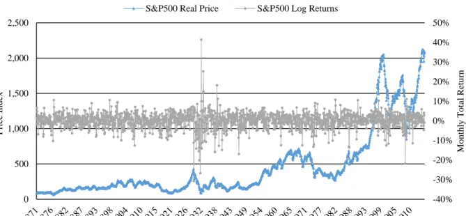
The aim of this paper is to focus on extreme returns, more specifically, very rare events, which makes it necessary to obtain a long time-series, including possible explanatory variables that have been identified above. Therefore, the only applicable time-series is the monthly S&P500 time-series which goes back to January 1871 until December 2015, including nominal and real dividends and earnings, from which the two ratios, dividend-yield and price-earnings-ratio can be computed.5 Information on data construction can be found in Shiller (1989). Overall, the time-series consists of 1,740 monthly price observations, which are used to calculate monthly log returns. Figure 1 depicts the time-series of the real prices as well as the log returns. As can be seen, real prices have been below 500 for the majority of the period until the 1960s, but grew remarkably for the latter 50 years. Crisis periods, e.g. the times for which one would expect extreme returns can be seen by the negative spikes of the grey line. Moreover, the log return series shows a fluctuation around a mean of zero, which is also depicted below in Table I together with the remaining descriptive statistics. Average monthly returns are 0.18%, and monthly volatility has been calculated to be 4.10%, which represents a modest yearly standard

(17)

deviation for equities of 14.20%. Additionally, the highest gain in one month was 41.48%, while the highest loss was 30.75%.

Figure 1: Historical S&P500 Prices and Log-Returns.

The figure shows the development of the S&P500 in real prices (blue) and its corresponding real log returns (grey) for each year between 1871 and 2015.

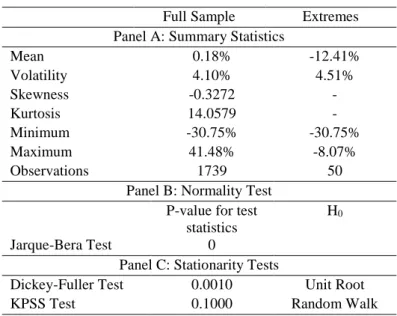
To apply the EVT-methodology, it is advisable to first test whether the approach is appropriate to the data in use, more specifically, whether the necessary conditions to apply the Hill-estimator are met. Starting with the stationarity of returns, a Dickey-Fuller (DF) test, as well as a Kwiatkowski–Phillips–Schmidt–Shin (KPSS) test are applied. Under the DF test the null hypothesis states that there is a unit root, e.g. the time-series is not stationary, while the alternative hypothesis states that there is no indication of non-stationarity (Dickey and Fuller 1979). The KPSS test is constructed the other way round and under its null, we can reject the case of a unit root and thus non-stationarity (Kwiatkowski et al. 1992).6 Applying both tests, yields clear results of stationarity of the return series as outlined in Table I below. This confirms

6_{For a thorough treatment on the subject, the interested reader might refer to the quoted articles.}

-40% -30% -20% -10% 0% 10% 20% 30% 40% 50% 0 500 1,000 1,500 2,000 2,500 Year M o n th ly T o tal Re tu rn P rice In d ex

(18)

what can be drawn optically from the plot in Figure 1 The log return series is stationary around its zero-mean.

Table I – Summary statistics

Full Sample Extremes

Panel A: Summary Statistics

Mean 0.18% -12.41% Volatility 4.10% 4.51% Skewness -0.3272 - Kurtosis 14.0579 - Minimum -30.75% -30.75% Maximum 41.48% -8.07% Observations 1739 50

Panel B: Normality Test P-value for test

statistics

H0

Jarque-Bera Test 0

Panel C: Stationarity Tests

Dickey-Fuller Test 0.0010 Unit Root

KPSS Test 0.1000 Random Walk

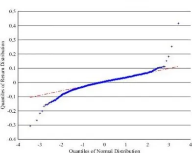
Next, it is assessed whether the return series meets the leptokurtic behaviour to be treated by EVT. Starting with a quantile-quantile-plot (QQ-plot) gives optical insights (Beirlant et al. 2006). A QQ-plot is based on an eye-test, thus checking whether the sample population fits a standard example distribution. Figure 2 below shows the empirical monthly returns fitted through a linear regression with the standard normal distribution. As can be seen, both tails deviate remarkably from the theoretical line of the standard normal distribution. Moreover, taking descriptive statistics in Table I into account, highly leptokurtic returns are evident with an excess kurtosis of 14.06. Moreover, the negative skewness of -0.33 indicates that more probability mass is cumulated in the left tail, a stylized fact for financial data, known as loss-asymmetry (Kahneman and Tversky 1979). Ultimately, a Jarque-Bera test for normality is conducted (Jarque and Bera 1987) and the results are tabulated in Table I as well. The test clearly rejects the null hypothesis of being normally distributed at the 1% significance-level, strongly confirming the precedent analyses. Overall, the evaluation points to non-normality and fat tails and thus allows to estimate the tail index 𝛼 by the means of the Hill-estimator.

(19)

Figure 2: QQ-Plot of S&P500 return series against the standard normal distribution

The plot shows the leptokurtic behaviour of the empirically observed returned series through the deviations from the linear line, which depicts the standard normal distribution.

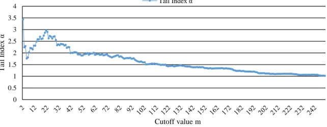
After confirming the necessary preconditions, the first step in preparing the data for EVT and to derive the Hill plot, is to sort these monthly returns from the lowest (e.g. the highest overall loss) to the highest. The lowest return gets the cut-off value m = 1, the second lowest receives the value m = 2 and so forth. Now, equation (1) serves as the applicable tool to estimate the tail-indices α, by inserting the returns lower than the cut-off value in the nominator and dividing it through the return corresponding to the cut-off value in the denominator. Taking the natural logarithm of the resulting fractions and summing them up yields a value of α which depends on m. Plotting α against m results in the Figure 3. The plot shows that in the beginning (low values for m), the variance is extremely high and the value of α fluctuates a lot, while for higher values of m the resulting curve becomes essentially flat, which represents the biasedness as more and more less extreme returns are included in the estimation of the tail-index parameter. Thus, using the eye-test, a cut-off value of m = 50 seems appropriate, implying an α equal to 1.81057. Assigning the value 1 to each of these 50 returns prepares the unsorted time-series for the application of the probit-model and defines the dependent variable Y. Descriptive statistics for the extreme part of the sample are depicted in Table I, as well.

(20)

Figure 3: Hill-Plot

The graph shows the different values for the tail-index α depending on the selected cut-off value m. The plot moves from an unstable pattern to a flat line when m increases.

Now, the construction of the explanatory variable is conducted. For this paper the dividend-yield was selected as it has more explanatory power and has been proven that it is less volatile compared to the E/P-ratio (Fama and French 1988). The dividend-yield is constructed by taking the real price and the real dividend, therefore including the inflation-deflator. It is calculated by using the following formula with dividends summed up over the last twelve months divided by this month’s price (Lewellen 2004), thus a moving sum of dividends:

𝐷𝑌𝑡 =

∑12_𝑖=1𝐷_𝑡−𝑖 𝑃𝑡

(13) As Campbell and Shiller (1998) point out, it has been empirically observed that the prices adjust back (and not dividends themselves) to average levels when this valuation ratio is far away from its normal level. As an example, a very low value for the dividend-yield signals either low dividend payments over the previous twelve months or a very high price. Given the fact that dividends are relatively stable, it can be assumed that it is the stock price which is extraordinary high and is therefore expected to decrease. Taking into account that markets tend to overreact in case of bad news or price corrections, makes a large sudden drop possible. When evaluating the time series trend of the dividend-yield, it appears that low values (e.g. high stock prices in the denominator) are indeed followed by large price movements: for instance, the financial

0 0.5 1 1.5 2 2.5 3 3.5 4 T ail In d ex α Cutoff value m Tail Index α

(21)

crisis 2008 with its initial loss of more than 20% in September, indeed showed some extremely low dividend-yield-values, meaning that stock prices were inflated. The same holds for the dotcom bubble in 2001 with a loss of 9.86% in March, which was led by the lowest values of the dividend-yield over the entire horizon. Likewise, the same pattern applies to the Great Depression in the 1930, which was preceded by a large and long-lasting decline in the dividend-yield. Thus, it might be a reasonable choice as explanatory variable.

6. Empirical Results

To obtain in-sample results the dependent variable will be regressed on the model specifications outlined above. The lag-length for the estimation was set from one to twelve for k and i, which results in the loss of those twelve observation of y at the beginning of the sample, reducing it effectively to 1,727 (lag = 1) until 1,716 (lag =12), respectively. The autoregressive term 𝜋_𝑡 remains fixed at the first lag. For both the pure dynamic and the autoregressive dynamic model this results in 144 different specifications, while for the static and pure autoregressive 12 different models are obtained.

6.1 Static Model

Starting with the static model, Table II shows that the model performs poorly in forecasting an extreme return with values for R² which are in the range between -0.74% and 1.20%. Statistical significance can be assessed from the standard errors, using a two-sided t-test (Wooldridge 2010). Both coefficients, the constant and 𝛽1 are significant for the lags one to four on a, at

least, 95%-significance level, thus indicating some explanatory power. However, for the fifth until the twelfth lag, 𝛽₁ loses its significance. 𝛽₁′𝑠 positive sign can be generally expected, as it increases the value of the linear estimator of 𝜋_𝑡 (e.g. the z-value) and consequently the probability to observe an extreme return. Contrary, the negative sign for the constant basically represents a very low probability of observing an extreme return alone, as this negative value applied to the cumulative distribution function of the standard normal distribution ends up in a

(22)

probability close to zero. Among the twelve specifications, the first lag provides the best in-sample fit, confirmed by the highest R. Generally, the static model is consistently estimated by all three in-sample criteria (R², AIC, and BIC), as ranking the model based on each criterion would result in an equal ranking.

Table II – Estimation Results – Static Model

The table entries R²-values for the model 𝑃𝑡−1(𝑦𝑡= 1)Φ(𝜋𝑡) = Φ(𝜔 + ∑12𝑘=1𝛽1∗ 𝑔𝑡−𝑘) where g depicts the

explanatory variable (DY). Moreover, it shows the coefficients’ estimates. The lag-length for DY is defined through k which varies from 1 to 12. Standard errors are reported in parentheses. * Represents significance level at 10%. ** Represents significance level at 5% *** Represents significance level at 1%.

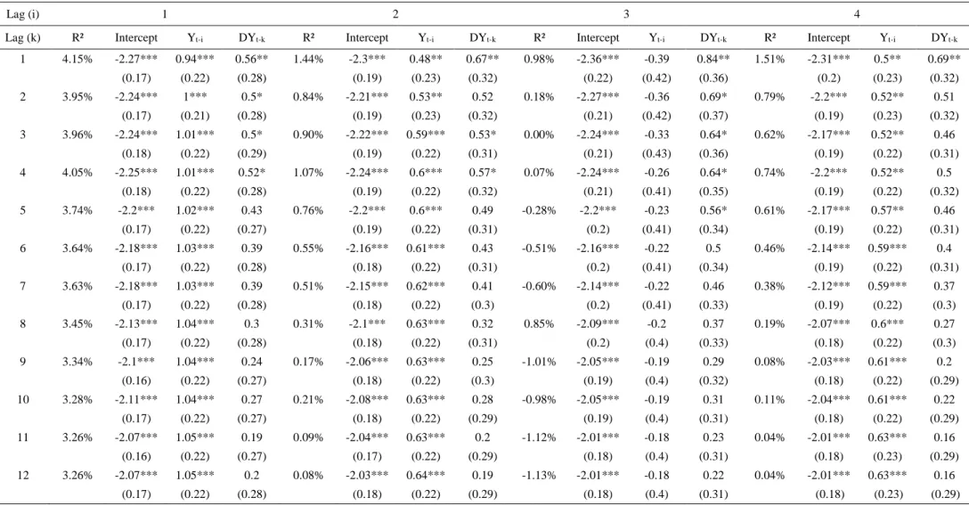
6.2 Pure Dynamic Model

Introducing the dynamic feature, the lagged dummy variable of whether or not an extreme return has been observed, 𝑦_𝑡−𝑖 produces the pure dynamic model. In general, the model improves on the one hand compared to the static one explained above, as R² reaches values up to 4.15%, but on the other hand, it reaches even lower values with the trough at -1.13%. However, it has to be stressed that this increase in R² might be also partly attributed to the increased number of explanatory variables as the inclusion of additional variables usually increases this measure. Among the 144 specifications, the model using the first lag of both, dividend-yield-ratio and extreme return dummy, clearly stands out with the highest R² (4.15%). Looking specifically at the coefficients of this specification, the picture from the static model is somewhat confirmed: the constant is highly significant at the 1%-level, while the

dividend-Lag (k) R² Intercept DYt-k Lag (k) R² Intercept DYt-k

1 1.20% -2.34*** 0.78** 7 -0.22% -2.14*** 0.45 (0.2) (0.33) (0.19) (0.32) 2 0.44% -2.25*** 0.63* 8 -0.46% -2.09*** 0.36 (0.2) (0.34) (0.19) (0.32) 3 0.30% -2.22*** 0.59* 9 -0.62% -2.05*** 0.29 (0.2) (0.34) (0.19) (0.31) 4 0.42% -2.24*** 0.62* 10 -0.59% -2.06*** 0.30 (0.2) (0.34) (0.19) (0.31) 5 0.09% -2.2*** 0.55 11 -0.72% -2.02*** 0.24 (0.2) (0.33) (0.18) (0.3) 6 -0.13% -2.16*** 0.48 12 -0.74% -2.01*** 0.23 (0.2) (0.33) (0.18) (0.31)

(23)

yield is merely significant for its first lag at the 5%-level and for some specifications at the 10%-level up until the fifth lag. The extreme return dummy variable exhibits more statistical power within this specification: for 99 out of 144 specifications the coefficients are significant, with the majority even at the 1%-level. Moreover, the first and second lag are both highly significant with 22 out of 24 reaching the 1%-level. Clearly, the model confirms a clustering of extreme events at this point as the coefficient seems to forecast an extreme event for the next, and the month after next, if a crash has been observed this month. Looking Figure 1 above, it can be observed that clustering is present in the 1930s, with an extreme series of three consecutive months (April to June 1932). Evaluating the coefficient’s sign, reveals that it is positive for all 144 specifications, confirming the hypothesis set out, that an extreme event dramatically increases the odds for a successive extreme event. The remaining coefficients are negative (constant), which again results in a very low natural level for the estimated probability, and positive (dividend-yield) over the entire range of models, which is in line with the observations of the static model.

(24)

Table III – Estimation Results – Pure Dynamic Model

The table entries R²-values for the model 𝑃𝑡−1(𝑦𝑡= 1)Φ(𝜋𝑡) = Φ(𝜔 + ∑𝑘𝑘=1𝛽1∗ 𝑔𝑡−𝑘+ ∑𝑖𝑖=1𝛽2∗ 𝑦𝑡−𝑖) where g depicts the explanatory variable (DY) and 𝑦𝑡−𝑖 represents

the lagged extreme return dummy. Moreover, it shows the coefficients’ estimates. The lag-length for DY is defined through k which varies from 1 to 12, while the lag-order for

𝑦𝑡−𝑖.is defined through i, which also varies from 1 to 12. Standard errors are reported in parentheses. * Represents significance level at 10%. ** Represents significance level

at 5% *** Represents significance level at 1%.

Lag (i) 1 2 3 4

Lag (k) R² Intercept Yt-i DYt-k R² Intercept Yt-i DYt-k R² Intercept Yt-i DYt-k R² Intercept Yt-i DYt-k

1 4.15% -2.27*** 0.94*** 0.56** 1.44% -2.3*** 0.48** 0.67** 0.98% -2.36*** -0.39 0.84** 1.51% -2.31*** 0.5** 0.69** (0.17) (0.22) (0.28) (0.19) (0.23) (0.32) (0.22) (0.42) (0.36) (0.2) (0.23) (0.32) 2 3.95% -2.24*** 1*** 0.5* 0.84% -2.21*** 0.53** 0.52 0.18% -2.27*** -0.36 0.69* 0.79% -2.2*** 0.52** 0.51 (0.17) (0.21) (0.28) (0.19) (0.23) (0.32) (0.21) (0.42) (0.37) (0.19) (0.23) (0.32) 3 3.96% -2.24*** 1.01*** 0.5* 0.90% -2.22*** 0.59*** 0.53* 0.00% -2.24*** -0.33 0.64* 0.62% -2.17*** 0.52** 0.46 (0.18) (0.22) (0.29) (0.19) (0.22) (0.31) (0.21) (0.43) (0.36) (0.19) (0.22) (0.31) 4 4.05% -2.25*** 1.01*** 0.52* 1.07% -2.24*** 0.6*** 0.57* 0.07% -2.24*** -0.26 0.64* 0.74% -2.2*** 0.52** 0.5 (0.18) (0.22) (0.28) (0.19) (0.22) (0.32) (0.21) (0.41) (0.35) (0.19) (0.22) (0.32) 5 3.74% -2.2*** 1.02*** 0.43 0.76% -2.2*** 0.6*** 0.49 -0.28% -2.2*** -0.23 0.56* 0.61% -2.17*** 0.57** 0.46 (0.17) (0.22) (0.27) (0.19) (0.22) (0.31) (0.2) (0.41) (0.34) (0.19) (0.22) (0.31) 6 3.64% -2.18*** 1.03*** 0.39 0.55% -2.16*** 0.61*** 0.43 -0.51% -2.16*** -0.22 0.5 0.46% -2.14*** 0.59*** 0.4 (0.17) (0.22) (0.28) (0.18) (0.22) (0.31) (0.2) (0.41) (0.34) (0.19) (0.22) (0.31) 7 3.63% -2.18*** 1.03*** 0.39 0.51% -2.15*** 0.62*** 0.41 -0.60% -2.14*** -0.22 0.46 0.38% -2.12*** 0.59*** 0.37 (0.17) (0.22) (0.28) (0.18) (0.22) (0.3) (0.2) (0.41) (0.33) (0.19) (0.22) (0.3) 8 3.45% -2.13*** 1.04*** 0.3 0.31% -2.1*** 0.63*** 0.32 0.85% -2.09*** -0.2 0.37 0.19% -2.07*** 0.6*** 0.27 (0.17) (0.22) (0.28) (0.18) (0.22) (0.31) (0.2) (0.4) (0.33) (0.18) (0.22) (0.3) 9 3.34% -2.1*** 1.04*** 0.24 0.17% -2.06*** 0.63*** 0.25 -1.01% -2.05*** -0.19 0.29 0.08% -2.03*** 0.61*** 0.2 (0.16) (0.22) (0.27) (0.18) (0.22) (0.3) (0.19) (0.4) (0.32) (0.18) (0.22) (0.29) 10 3.28% -2.11*** 1.04*** 0.27 0.21% -2.08*** 0.63*** 0.28 -0.98% -2.05*** -0.19 0.31 0.11% -2.04*** 0.61*** 0.22 (0.17) (0.22) (0.27) (0.18) (0.22) (0.29) (0.19) (0.4) (0.31) (0.18) (0.22) (0.29) 11 3.26% -2.07*** 1.05*** 0.19 0.09% -2.04*** 0.63*** 0.2 -1.12% -2.01*** -0.18 0.23 0.04% -2.01*** 0.63*** 0.16 (0.16) (0.22) (0.27) (0.17) (0.22) (0.29) (0.18) (0.4) (0.31) (0.18) (0.23) (0.29) 12 3.26% -2.07*** 1.05*** 0.2 0.08% -2.03*** 0.64*** 0.19 -1.13% -2.01*** -0.18 0.22 0.04% -2.01*** 0.63*** 0.16 (0.17) (0.22) (0.28) (0.18) (0.22) (0.29) (0.18) (0.4) (0.31) (0.18) (0.23) (0.29)

(25)

Table III- continued

Lag (i) 5 6 7 8

1 1.09% -2.31*** 0.35 0.72** 2.65% -2.29*** 0.74*** 0.63** 2.63% -2.29*** 0.74*** 0.62** 1.90% -2.28*** 0.6*** 0.64** (0.2) (0.28) (0.31) (0.19) (0.22) (0.31) (0.19) (0.24) (0.3) (0.19) (0.22) (0.3) 2 0.40% -2.22*** 0.39 0.56* 2.07% -2.2*** 0.78*** 0.47 2.11% -2.21*** 0.78*** 0.48 1.33% -2.19*** 0.65*** 0.48 (0.19) (0.28) (0.32) (0.19) (0.22) (0.31) (0.19) (0.24) (0.3) (0.18) (0.22) (0.3) 3 0.22% -2.19*** 0.37 0.51 1.93% -2.17*** 0.78*** 0.42 2.03% -2.19*** 0.79*** 0.45 1.29% -2.18*** 0.67*** 0.46 (0.19) (0.29) (0.31) (0.19) (0.21) (0.3) (0.19) (0.24) (0.31) (0.19) (0.23) (0.31) 4 0.31% -2.21*** 0.35 0.53* 1.96% -2.18*** 0.77*** 0.43 1.81% -2.14*** 0.79*** 0.37 1.40% -2.2*** 0.66*** 0.49 (0.19) (0.29) (0.32) (0.18) (0.22) (0.3) (0.18) (0.25) (0.3) (0.19) (0.23) (0.31) 5 0.05% -2.16*** 0.39 0.46 1.74% -2.13*** 0.79*** 0.34 1.67% -2.11*** 0.8*** 0.3 1.12% -2.15*** 0.68*** 0.4 (0.19) (0.29) (0.31) (0.18) (0.22) (0.29) (0.18) (0.25) (0.29) (0.18) (0.23) (0.3) 6 -0.05% -2.14*** 0.45 0.42 1.64% -2.1*** 0.81*** 0.29 1.65% -2.1*** 0.81*** 0.28 0.92% -2.1*** 0.69*** 0.31 (0.19) (0.28) (0.31) (0.18) (0.22) (0.28) (0.18) (0.25) (0.29) (0.18) (0.23) (0.29) 7 -0.08% -2.13*** 0.46 0.4 1.76% -2.13*** 0.83*** 0.34 1.65% -2.1*** 0.81*** 0.28 0.83% -2.07*** 0.69*** 0.26 (0.19) (0.29) (0.3) (0.18) (0.22) (0.29) (0.18) (0.25) (0.29) (0.17) (0.23) (0.27) 8 -0.29% -2.08*** 0.47 0.31 1.61% -2.09*** 0.84*** 0.26 1.63% -2.09*** 0.84*** 0.27 0.72% -2.03*** 0.72*** 0.18 (0.19) (0.29) (0.31) (0.19) (0.22) (0.3) (0.19) (0.25) (0.3) (0.18) (0.23) (0.28) 9 -0.43% -2.04*** 0.48* 0.23 1.50% -2.05*** 0.85*** 0.19 1.54% -2.07*** 0.85*** 0.22 0.71% -2.02*** 0.74*** 0.16 (0.18) (0.29) (0.29) (0.18) (0.23) (0.29) (0.18) (0.25) (0.3) (0.18) (0.24) (0.28) 10 -0.40% -2.05*** 0.48* 0.25 1.51% -2.05*** 0.85*** 0.2 1.56% -2.07*** 0.85*** 0.24 0.74% -2.04*** 0.74*** 0.2 (0.18) (0.29) (0.29) (0.18) (0.23) (0.28) (0.18) (0.25) (0.29) (0.18) (0.24) (0.28) 11 -0.50% -2.01*** 0.49* 0.18 1.44% -2.02*** 0.85*** 0.14 1.46% -2.03*** 0.85*** 0.15 0.67% -2*** 0.75*** 0.12 (0.18) (0.29) (0.29) (0.18) (0.23) (0.28) (0.18) (0.25) (0.29) (0.17) (0.24) (0.28) 12 -0.50% -2.01*** 0.49* 0.17 1.44% -2.02*** 0.85*** 0.14 1.45% -2.03*** 0.85*** 0.15 0.66% -1.99*** 0.75*** 0.1 (0.18) (0.3) (0.29) (0.18) (0.23) (0.29) (0.18) (0.25) (0.29) (0.18) (0.24) (0.28)

(26)

Table III- continued

Lag (i) 9 10 11 12

1 0.81% -2.32*** 0.13 0.76** 1.15% -2.32*** 0.37 0.72** 1.15% -2.32*** 0.37 0.73** 2.05% -2.3*** 0.63*** 0.67** (0.2) (0.26) (0.33) (0.2) (0.3) (0.34) (0.2) (0.27) (0.32) (0.19) (0.23) (0.31) 2 0.08% -2.23*** 0.18 0.59* 0.43% -2.22*** 0.39 0.56 0.43% -2.22*** 0.39 0.56* 1.39% -2.2*** 0.66*** 0.5 (0.2) (0.26) (0.33) (0.2) (0.3) (0.34) (0.19) (0.27) (0.32) (0.19) (0.23) (0.3) 3 -0.03% -2.21*** 0.21 0.55* 0.27% -2.2*** 0.39 0.52 0.30% -2.2*** 0.4 0.52 1.22% -2.17*** 0.66*** 0.44 (0.2) (0.25) (0.33) (0.2) (0.29) (0.34) (0.19) (0.27) (0.32) (0.18) (0.23) (0.3) 4 0.09% -2.23*** 0.22 0.59* 0.38% -2.22*** 0.38 0.55 0.41% -2.22*** 0.4 0.55* 1.30% -2.19*** 0.65*** 0.46 (0.2) (0.25) (0.33) (0.2) (0.29) (0.35) (0.19) (0.27) (0.32) (0.19) (0.23) (0.3) 5 -0.22% -2.18*** 0.24 0.51 0.12% -2.17*** 0.42 0.48 0.13% -2.17*** 0.42 0.47 1.06% -2.14*** 0.67*** 0.38 (0.19) (0.25) (0.32) (0.2) (0.28) (0.34) (0.19) (0.27) (0.32) (0.18) (0.23) (0.29) 6 -0.43% -2.14*** 0.25 0.44 -0.07% -2.14*** 0.43 0.41 -0.04% -2.14*** 0.44* 0.42 0.93% -2.1*** 0.69*** 0.32 (0.19) (0.25) (0.32) (0.19) (0.28) (0.34) (0.19) (0.26) (0.32) (0.18) (0.23) (0.29) 7 -0.53% -2.12*** 0.25 0.39 -0.15% -2.12*** 0.44 0.38 -0.10% -2.13*** 0.45* 0.39 0.91% -2.1*** 0.7*** 0.3 (0.19) (0.25) (0.31) (0.19) (0.28) (0.32) (0.19) (0.27) (0.32) (0.18) (0.24) (0.29) 8 -0.74% -2.07*** 0.26 0.3 -0.37% -2.06*** 0.45 0.27 -0.31% -2.08*** 0.46* 0.3 0.77% -2.05*** 0.72*** 0.22 (0.18) (0.25) (0.31) (0.19) (0.28) (0.32) (0.19) (0.27) (0.32) (0.19) (0.24) (0.31) 9 -0.86% -2.03*** 0.29 0.23 -0.48% -2.02*** 0.46* 0.19 -0.45% -2.03*** 0.47* 0.21 0.68% -2.01*** 0.73*** 0.14 (0.18) (0.26) (0.3) (0.18) (0.28) (0.3) (0.18) (0.27) (0.31) (0.18) (0.24) (0.29) 10 -0.81% -2.05*** 0.31 0.26 -0.46% -2.03*** 0.46* 0.21 -0.44% -2.04*** 0.47* 0.22 0.68% -2*** 0.73*** 0.13 (0.18) (0.26) (0.3) (0.18) (0.28) (0.3) (0.18) (0.27) (0.3) (0.18) (0.25) (0.29) 11 -0.91% -2.01*** 0.33 0.19 -0.50% -2.01*** 0.49* 0.17 -0.52% -2*** 0.48* 0.15 0.63% -1.96*** 0.75*** 0.04 (0.18) (0.26) (0.29) (0.18) (0.27) (0.3) (0.18) (0.27) (0.3) (0.17) (0.25) (0.28) 12 -0.92% -2*** 0.33 0.18 -0.51% -2.01*** 0.49* 0.17 -0.50% -2.01*** 0.49* 0.18 0.64% -1.96*** 0.75*** 0.05 (0.18) (0.26) (0.29) (0.18) (0.27) (0.3) (0.18) (0.26) (0.3) (0.17) (0.25) (0.28)

(27)

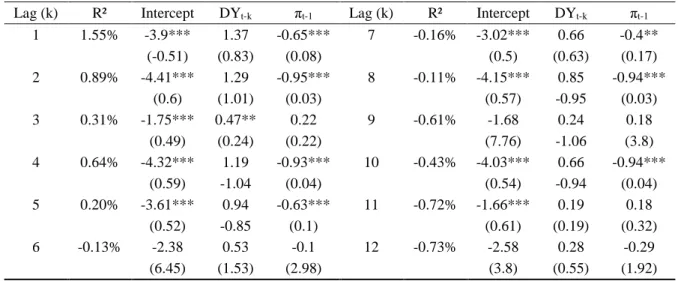
6.3 Pure Autoregressive Model

The next model to be assessed is the pure autoregressive, which introduces the lagged structure of 𝜋_𝑡. Contrary, to the dynamic model it is worth highlighting that in this model the term 𝜋_𝑡−1 has been fixed to the first lag, which overall results in 12 specifications, as only the dividend-yield is again lagged until its twelfth’s value. Generally, the in-sample fit improves slightly compared to the static model with R² values ranging from -0.73 to 1.55%, depicted by Table IV. Although this is not significantly higher, it has to be stressed that each lag is superior to its corresponding lag from the static model (e.g. first lag R² is higher for the autoregressive, as compared to the first lag of the static). Nevertheless, it also exploits one additional variable, which should generally increase R². Comparing it to the dynamic model, which uses the same number of coefficients shows a significantly lower value. When looking at the significance of the coefficients a different picture from the two previously assessed models emerges: the dividend-yield is merely significant for its third lag at the (5%-level), while also the constant loses significance for the sixth, ninth, and twelfth lag. For these three specifications none of the explanatory variables reaches any significance level. However, the intercept’s loss of significance for the three lags of the dividend-yield means that it is indeed equal to zero, which results in an overall higher natural level for the probability, because the linear estimator gets less negative. The autoregressive feature 𝜋_𝑡−1 is significant at the 1%-level for six out of twelve specifications, while it is not significant for 5 cases. Moreover, it bears a negative sign for all significant specifications. Initially, this result does not seem intuitive, but it should be pointed out, that the value of 𝜋_𝑡 is in general below zero, as it is linearly estimated with a negative constant, which is in absolute terms approximately threefold the value of the dividend-yield for this model. Consequently, that 𝜋_𝑡 ends up being positive, and thus increasing the probability of an extreme event through a higher z-value, the value for the dividend-yield would need to be around 3 (leaving out the effect of 𝜋𝑡−1 for simplicity), but its maximum value merely reaches

(28)

1.90, which occurred around the time of the great depression in June 1932. Even the initial value 𝜋0 is negative as it is estimated by the coefficients times the time-series mean, as well as

the highly negative constant. Therefore, the negative sign can be expected from econometric modelling viewpoints. Nevertheless, while it is puzzling why the sign changes for the third lag (negative constant), it gets clear that the positive sign for the sixth and the eleventh lag is in line with the zero intercept explained above which renders the z-value positive and thus 𝜋_𝑡−1 needs to have a positive sign to increase the probability.

Table IV – Estimation Results – Pure Autoregressive Model

The table entries R²-values for the model 𝑃𝑡−1(𝑦𝑡= 1)Φ(𝜋𝑡) = Φ(𝜔 + 𝛼 ∗ 𝜋𝑡−1+ ∑𝑘=112 𝛽1∗ 𝑔𝑡−𝑘) where g

depicts the explanatory variable (DY) and 𝜋𝑡−1 introduces the autoregressive feature Moreover, it shows the

coefficients’ estimates. The lag-length for DY is defined through k which varies from 1 to 12. Standard errors are reported in parentheses. * Represents significance level at 10%. ** Represents significance level at 5% *** Represents significance level at 1%.

Lag (k) R² Intercept DYt-k πt-1 Lag (k) R² Intercept DYt-k πt-1

1 1.55% -3.9*** 1.37 -0.65*** 7 -0.16% -3.02*** 0.66 -0.4** (-0.51) (0.83) (0.08) (0.5) (0.63) (0.17) 2 0.89% -4.41*** 1.29 -0.95*** 8 -0.11% -4.15*** 0.85 -0.94*** (0.6) (1.01) (0.03) (0.57) -0.95 (0.03) 3 0.31% -1.75*** 0.47** 0.22 9 -0.61% -1.68 0.24 0.18 (0.49) (0.24) (0.22) (7.76) -1.06 (3.8) 4 0.64% -4.32*** 1.19 -0.93*** 10 -0.43% -4.03*** 0.66 -0.94*** (0.59) -1.04 (0.04) (0.54) -0.94 (0.04) 5 0.20% -3.61*** 0.94 -0.63*** 11 -0.72% -1.66*** 0.19 0.18 (0.52) -0.85 (0.1) (0.61) (0.19) (0.32) 6 -0.13% -2.38 0.53 -0.1 12 -0.73% -2.58 0.28 -0.29 (6.45) (1.53) (2.98) (3.8) (0.55) (1.92)

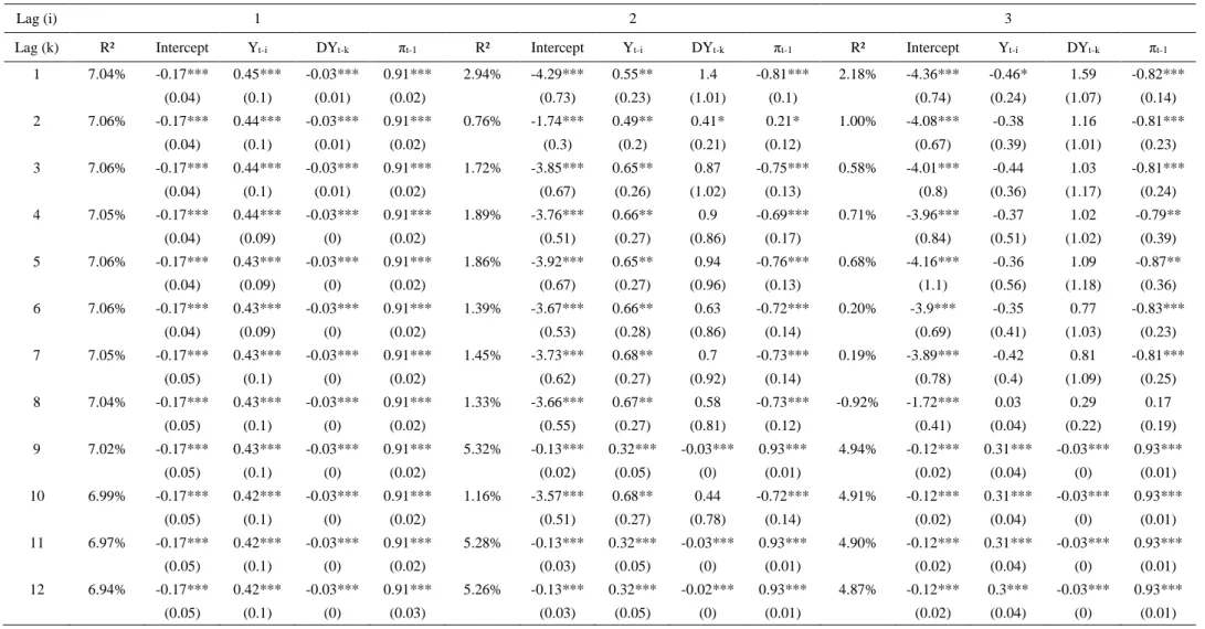
6.4 Dynamic Autoregressive Model

The last specification to evaluate is the dynamic autoregressive specification which combines both the autoregressive (𝜋_𝑡−1) and the dynamic feature (𝑦_𝑡−𝑖). Similarly, to the pure autoregressive model, 𝜋_𝑡−1 is fixed to the first lag, while the extreme return dummy and the dividend-yield vary from one to twelve, resulting again in 144 different specifications. Starting with the overall model performance it can be observed that the in-sample fit clearly improves with R² ranging from -0.92% to 7.06%, which is more than 5 times better than the best static

(29)

model. The best performance with this specification is provided by the model exploiting the second, third, fifth and sixth lag of the dividend-yield and always the first lag of the extreme return dummy, respectively. Comparing the four coefficients to the previously applied models now results in a different picture, except for the constant which is again highly significant for all 144 specifications at the 1%-level: the lagged extreme return dummy possesses notably higher relevance in this model as it is insignificant in only eight instances. From the remaining 136 models, the majority is at the 1%-level (125). The main explanatory variable, the dividend-yield, is remarkably more important within this specification, as it reaches the 1% significance level in 123 cases, while it is insignificant in only 18 instances. Lastly, the autoregressive feature even reaches the 1%-level for 138 specifications, with extremely high t-statistics, indicating its high relevance. Interestingly, among all three variables the non-significant cases are cumulated in the third lag of the extreme return dummy. This interpretation is somewhat unclear as all coefficients return back to its high significance for any longer lag length. However, when looking at the coefficients’ sign, the constant bears a negative sign again, while the extreme return dummy is basically positive (except for the non-significant instances). Returning to the hypothesis from the pure dynamic model, this confirms the extremal clustering in the series, explained above. Interestingly, the dividend-yield is negative for this model specification over the entire range. This can be interpreted as working against the lagged extreme dummy, as the linear estimator 𝜋_𝑡−1 will be moved further into negative territory, thus decreasing the z-value applied to the cumulative distribution function. This is somewhat unexpected, as asset pricing theory attributed explanatory power to the dividend-yield in forecasting equity returns. However, in this case, the negative sign clearly decreases the probability of observing an extreme price movement. Additionally, the reversal of the coefficients compared to the autoregressive model also holds for 𝜋_𝑡−1, which exhibits a positive sign now. The interpretation is not easily drawn in this case but an explanation might be already

(30)

pointed out from Kauppi and Saikkonen (2008), who conclude that the term 𝜋_𝑡−1 possibly act in a complicated way with the explanatory variables.

6.5 Discussion of the Results

As the previous findings are somewhat hard to grasp, a brief summary is provided at this point. First, the intercept in each of the models is generally significant and negative which results in a low natural level of the estimated probabilities of observing an extreme price movement. The dividend-yield reveals mixed findings, as it is not relevant at all for the pure dynamic model, while it is very relevant for the dynamic autoregressive model. Moreover, it changes sign across different models, which makes it hard to interpret. The lagged extreme dummy variable shows by far the clearest results: it is relevant in both models, and highly confirms the research hypothesis of extremal clustering. Compared to the dividend-yield its direction is very consistent, as it is on the one hand strictly positive with values around 0.30 to 0.98 and on the other hand merely insignificant. The autoregressive term is in general also extremely relevant, outlined by its t-statistics which are as high as approximately 97. The behaviour is nevertheless somewhat hard to interpret as it changes sign and thus sometimes decreases the probability of observing an extreme return. However, the second research hypothesis, whether the dynamic modelling approach improves the performance of the static model can be confirmed as well at this point. Additionally, looking at the in-sample criterion R² this finding is undermined and the ultimate conclusion that both research hypotheses can be confirmed are drawn.

(31)

Table V – Estimation Results – Dynamic Autoregressive Model

The table entries R²-values for the model 𝑃𝑡−1(𝑦𝑡= 1)Φ(𝜋𝑡) = Φ(𝜔 +𝛼 ∗ 𝜋𝑡−1∑𝑘𝑘=1𝛽1∗ 𝑔𝑡−𝑘+ ∑𝑖𝑖=1𝛽2∗ 𝑦𝑡−𝑖) where g depicts the explanatory variable (DY), 𝑦𝑡−𝑖 represents the lagged

extreme return dummy and 𝜋𝑡−1 stands for the autoregressive feature. Moreover, it shows the coefficients’ estimates. The lag-length for DY is defined through k which varies

from 1 to 12, while the lag-order for 𝑦𝑡−𝑖.is defined through i, which also varies from 1 to 12. Standard errors are reported in parentheses. * Represents significance level at

10%. ** Represents significance level at 5% *** Represents significance level at 1%.

Lag (i) 1 2 3

Lag (k) R² Intercept Yt-i DYt-k πt-1 R² Intercept Yt-i DYt-k πt-1 R² Intercept Yt-i DYt-k πt-1

1 7.04% -0.17*** 0.45*** -0.03*** 0.91*** 2.94% -4.29*** 0.55** 1.4 -0.81*** 2.18% -4.36*** -0.46* 1.59 -0.82*** (0.04) (0.1) (0.01) (0.02) (0.73) (0.23) (1.01) (0.1) (0.74) (0.24) (1.07) (0.14) 2 7.06% -0.17*** 0.44*** -0.03*** 0.91*** 0.76% -1.74*** 0.49** 0.41* 0.21* 1.00% -4.08*** -0.38 1.16 -0.81*** (0.04) (0.1) (0.01) (0.02) (0.3) (0.2) (0.21) (0.12) (0.67) (0.39) (1.01) (0.23) 3 7.06% -0.17*** 0.44*** -0.03*** 0.91*** 1.72% -3.85*** 0.65** 0.87 -0.75*** 0.58% -4.01*** -0.44 1.03 -0.81*** (0.04) (0.1) (0.01) (0.02) (0.67) (0.26) (1.02) (0.13) (0.8) (0.36) (1.17) (0.24) 4 7.05% -0.17*** 0.44*** -0.03*** 0.91*** 1.89% -3.76*** 0.66** 0.9 -0.69*** 0.71% -3.96*** -0.37 1.02 -0.79** (0.04) (0.09) (0) (0.02) (0.51) (0.27) (0.86) (0.17) (0.84) (0.51) (1.02) (0.39) 5 7.06% -0.17*** 0.43*** -0.03*** 0.91*** 1.86% -3.92*** 0.65** 0.94 -0.76*** 0.68% -4.16*** -0.36 1.09 -0.87** (0.04) (0.09) (0) (0.02) (0.67) (0.27) (0.96) (0.13) (1.1) (0.56) (1.18) (0.36) 6 7.06% -0.17*** 0.43*** -0.03*** 0.91*** 1.39% -3.67*** 0.66** 0.63 -0.72*** 0.20% -3.9*** -0.35 0.77 -0.83*** (0.04) (0.09) (0) (0.02) (0.53) (0.28) (0.86) (0.14) (0.69) (0.41) (1.03) (0.23) 7 7.05% -0.17*** 0.43*** -0.03*** 0.91*** 1.45% -3.73*** 0.68** 0.7 -0.73*** 0.19% -3.89*** -0.42 0.81 -0.81*** (0.05) (0.1) (0) (0.02) (0.62) (0.27) (0.92) (0.14) (0.78) (0.4) (1.09) (0.25) 8 7.04% -0.17*** 0.43*** -0.03*** 0.91*** 1.33% -3.66*** 0.67** 0.58 -0.73*** -0.92% -1.72*** 0.03 0.29 0.17 (0.05) (0.1) (0) (0.02) (0.55) (0.27) (0.81) (0.12) (0.41) (0.04) (0.22) (0.19) 9 7.02% -0.17*** 0.43*** -0.03*** 0.91*** 5.32% -0.13*** 0.32*** -0.03*** 0.93*** 4.94% -0.12*** 0.31*** -0.03*** 0.93*** (0.05) (0.1) (0) (0.02) (0.02) (0.05) (0) (0.01) (0.02) (0.04) (0) (0.01) 10 6.99% -0.17*** 0.42*** -0.03*** 0.91*** 1.16% -3.57*** 0.68** 0.44 -0.72*** 4.91% -0.12*** 0.31*** -0.03*** 0.93*** (0.05) (0.1) (0) (0.02) (0.51) (0.27) (0.78) (0.14) (0.02) (0.04) (0) (0.01) 11 6.97% -0.17*** 0.42*** -0.03*** 0.91*** 5.28% -0.13*** 0.32*** -0.03*** 0.93*** 4.90% -0.12*** 0.31*** -0.03*** 0.93*** (0.05) (0.1) (0) (0.02) (0.03) (0.05) (0) (0.01) (0.02) (0.04) (0) (0.01) 12 6.94% -0.17*** 0.42*** -0.03*** 0.91*** 5.26% -0.13*** 0.32*** -0.02*** 0.93*** 4.87% -0.12*** 0.3*** -0.03*** 0.93*** (0.05) (0.1) (0) (0.03) (0.03) (0.05) (0) (0.01) (0.02) (0.04) (0) (0.01)

(32)

Table V- continued

Lag (i) 4 5 6

1 5.87% -0.18*** 0.43*** -0.03*** 0.91*** 5.80% -0.19*** 0.45*** -0.03*** 0.9*** 6.17% -0.24*** 0.54*** -0.04*** 0.88*** (0.03) (0.06) (0.01) (0.01) (0.03) (0.06) (0.01) (0.01) (0.05) (0.1) (0.01) (0.03) 2 5.94% -0.17*** 0.43*** -0.04*** 0.91*** 5.87% -0.19*** 0.46*** -0.04*** 0.9*** 6.25% -0.23*** 0.54*** -0.05*** 0.88*** (0.02) (0.05) (0.01) (0.01) (0.03) (0.06) (0.01) (0.01) (0.05) (0.1) (0.01) (0.03) 3 5.97% -0.17*** 0.43*** -0.04*** 0.91*** 5.92% -0.19*** 0.46*** -0.04*** 0.9*** 6.30% -0.23*** 0.54*** -0.05*** 0.88*** (0.02) (0.05) (0.01) (0.01) (0.03) (0.06) (0.01) (0.01) (0.05) (0.1) (0.01) (0.03) 4 5.99% -0.17*** 0.43*** -0.04*** 0.91*** 5.94% -0.19*** 0.46*** -0.04*** 0.9*** 6.34% -0.23*** 0.54*** -0.05*** 0.88*** (0.02) (0.05) (0.01) (0.01) (0.03) (0.06) (0.01) (0.01) (0.05) (0.1) (0.01) (0.03) 5 6.00% -0.17*** 0.42*** -0.04*** 0.91*** 5.97% -0.18*** 0.46*** -0.04*** 0.9*** 6.39% -0.23*** 0.54*** -0.06*** 0.88*** (0.02) (0.05) (0.01) (0.01) (0.03) (0.06) (0.01) (0.01) (0.05) (0.1) (0.01) (0.03) 6 6.01% -0.17*** 0.42*** -0.04*** 0.91*** 5.97% -0.18*** 0.45*** -0.04*** 0.9*** 6.41% -0.22*** 0.54*** -0.06*** 0.88*** (0.02) (0.05) (0.01) (0.01) (0.03) (0.06) (0.01) (0.01) (0.05) (0.1) (0.01) (0.03) 7 6.00% -0.17*** 0.42*** -0.04*** 0.91*** 5.96% -0.18*** 0.45*** -0.04*** 0.9*** 6.38% -0.22*** 0.53*** -0.05*** 0.88*** (0.02) (0.05) (0) (0.01) (0.03) (0.06) (0.01) (0.01) (0.05) (0.1) (0.01) (0.03) 8 5.99% -0.17*** 0.41*** -0.04*** 0.91*** 5.96% -0.18*** 0.44*** -0.04*** 0.9*** 6.37% -0.22*** 0.52*** -0.05*** 0.88*** (0.02) (0.05) (0) (0.01) (0.03) (0.06) (0.01) (0.01) (0.05) (0.1) (0.01) (0.03) 9 5.97% -0.17*** 0.41*** -0.04*** 0.91*** 5.93% -0.18*** 0.44*** -0.04*** 0.9*** 6.34% -0.22*** 0.52*** -0.05*** 0.88*** (0.03) (0.05) (0) (0.01) (0.03) (0.06) (0) (0.01) (0.05) (0.1) (0.01) (0.03) 10 5.93% -0.17*** 0.4*** -0.04*** 0.91*** 5.90% -0.18*** 0.43*** -0.04*** 0.9*** 6.29% -0.22*** 0.51*** -0.05*** 0.88*** (0.03) (0.05) (0) (0.01) (0.03) (0.06) (0) (0.01) (0.05) (0.1) (0.01) (0.03) 11 5.91% -0.17*** 0.4*** -0.03*** 0.91*** 5.87% -0.18*** 0.43*** -0.04*** 0.9*** 6.27% -0.23*** 0.51*** -0.05*** 0.88*** (0.03) (0.05) (0) (0.01) (0.03) (0.06) (0) (0.01) (0.06) (0.1) (0.01) (0.03) 12 5.88% -0.17*** 0.4*** -0.03*** 0.91*** 5.84% -0.19*** 0.43*** -0.04*** 0.9*** 6.23% -0.23*** 0.51*** -0.04*** 0.88*** (0.03) (0.05) (0) (0.01) (0.03) (0.06) (0) (0.02) (0.06) (0.11) (0.01) (0.03)

(33)

Lag (i) 7 8 9

1 5.00% -0.21*** 0.46*** -0.03*** 0.89*** 2.20% -3.77*** 0.54* 1.21 -0.61* 0.75% -1.78*** 0.24 0.54*** 0.22 (0.05) (0.1) (0.01) (0.03) (0.84) (0.3) (0.78) (0.31) (0.61) (0.16) (0.2) (0.27) 2 5.08% -0.21*** 0.46*** -0.04*** 0.89*** 3.95% -0.18*** 0.38*** -0.03*** 0.91*** 3.29% -0.17*** 0.34*** -0.02*** 0.91*** (0.05) (0.1) (0.01) (0.02) (0.04) (0.07) (0.01) (0.02) (0.03) (0.06) (0) (0.02) 3 5.12% -0.2*** 0.46*** -0.04*** 0.89*** 4.00% -0.18*** 0.39*** -0.03*** 0.91*** 3.33% -0.16*** 0.35*** -0.03*** 0.91*** (0.05) (0.1) (0.01) (0.02) (0.03) (0.07) (0.01) (0.02) (0.03) (0.06) (0.01) (0.02) 4 5.17% -0.2*** 0.46*** -0.04*** 0.89*** 4.05% -0.17*** 0.39*** -0.04*** 0.91*** 3.38% -0.16*** 0.35*** -0.03*** 0.91*** (0.04) (0.1) (0.01) (0.02) (0.03) (0.07) (0.01) (0.02) (0.03) (0.06) (0.01) (0.01) 5 5.23% -0.2*** 0.47*** -0.05*** 0.89*** 4.11% -0.17*** 0.39*** -0.04*** 0.91*** 3.44% -0.16*** 0.35*** -0.03*** 0.91*** (0.04) (0.1) (0.01) (0.02) (0.03) (0.07) (0.01) (0.02) (0.03) (0.05) (0.01) (0.01) 6 5.27% -0.2*** 0.47*** -0.05*** 0.89*** 4.16% -0.17*** 0.39*** -0.04*** 0.91*** 3.50% -0.16*** 0.36*** -0.04*** 0.91*** (0.04) (0.1) (0.01) (0.02) (0.03) (0.07) (0.01) (0.02) (0.03) (0.05) (0.01) (0.01) 7 5.28% -0.2*** 0.46*** -0.05*** 0.89*** 4.19% -0.17*** 0.39*** -0.04*** 0.91*** 3.53% -0.16*** 0.36*** -0.04*** 0.91*** (0.04) (0.09) (0.01) (0.02) (0.03) (0.07) (0.01) (0.02) (0.03) (0.05) (0.01) (0.01) 8 5.28% -0.2*** 0.46*** -0.05*** 0.89*** 4.21% -0.17*** 0.39*** -0.04*** 0.91*** 3.57% -0.16*** 0.36*** -0.04*** 0.91*** (0.04) (0.09) (0.01) (0.02) (0.03) (0.07) (0.01) (0.02) (0.03) (0.05) (0.01) (0.01) 9 5.25% -0.2*** 0.45*** -0.05*** 0.9*** 4.19% -0.17*** 0.38*** -0.04*** 0.91*** 3.57% -0.16*** 0.35*** -0.04*** 0.92*** (0.04) (0.09) (0.01) (0.02) (0.03) (0.06) (0.01) (0.02) (0.03) (0.05) (0.01) (0.01) 10 5.21% -0.2*** 0.44*** -0.04*** 0.9*** 4.16% -0.17*** 0.38*** -0.04*** 0.91*** 3.55% -0.15*** 0.35*** -0.04*** 0.92*** (0.05) (0.09) (0.01) (0.02) (0.03) (0.06) (0.01) (0.02) (0.03) (0.05) (0.01) (0.01) 11 5.19% -0.2*** 0.44*** -0.04*** 0.9*** 4.14% -0.17*** 0.37*** -0.04*** 0.91*** 3.53% -0.15*** 0.34*** -0.04*** 0.92*** (0.05) (0.09) (0.01) (0.02) (0.03) (0.06) (0.01) (0.02) (0.03) (0.05) (0.01) (0.01) 12 5.16% -0.2*** 0.44*** -0.04*** 0.9*** 4.12% -0.17*** 0.37*** -0.04*** 0.91*** 3.51% -0.15*** 0.34*** -0.04*** 0.92*** (0.05) (0.09) (0.01) (0.02) (0.03) (0.06) (0.01) (0.02) (0.03) (0.05) (0.01) (0.01)

(34)

Lag (i) 10 11 12

1 3.46% -0.2*** 0.38*** -0.02** 0.9*** 3.44% -0.23*** 0.41*** -0.01* 0.88*** 3.41% -0.27*** 0.44*** -0.01 0.87*** (0.04) (0.07) (0.01) (0.02) (0.04) (0.07) (0.01) (0.02) (0.07) (0.1) (0.01) (0.03) 2 3.52% -0.2*** 0.39*** -0.02*** 0.9*** 3.50% -0.22*** 0.41*** -0.02*** 0.89*** 3.45% -0.25*** 0.44*** -0.02*** 0.87*** (0.04) (0.07) (0.01) (0.02) (0.04) (0.07) (0.01) (0.02) (0.06) (0.09) (0.01) (0.03) 3 3.58% -0.19*** 0.39*** -0.03*** 0.9*** 3.55% -0.21*** 0.42*** -0.03*** 0.89*** 3.50% -0.24*** 0.45*** -0.03*** 0.88*** (0.04) (0.07) (0.01) (0.02) (0.04) (0.07) (0.01) (0.02) (0.05) (0.09) (0.01) (0.03) 4 3.63% -0.19*** 0.39*** -0.03*** 0.9*** 3.61% -0.21*** 0.42*** -0.04*** 0.89*** 3.56% -0.23*** 0.45*** -0.04*** 0.88*** (0.04) (0.07) (0.01) (0.02) (0.03) (0.07) (0.01) (0.02) (0.05) (0.09) (0.01) (0.02) 5 3.70% -0.18*** 0.4*** -0.04*** 0.9*** 3.68% -0.2*** 0.43*** -0.04*** 0.89*** 3.65% -0.23*** 0.46*** -0.04*** 0.88*** (0.04) (0.07) (0.01) (0.02) (0.03) (0.07) (0.01) (0.02) (0.05) (0.09) (0.01) (0.02) 6 3.75% -0.18*** 0.4*** -0.04*** 0.9*** 3.75% -0.2*** 0.43*** -0.05*** 0.89*** 3.72% -0.22*** 0.47*** -0.05*** 0.88*** (0.03) (0.07) (0.01) (0.02) (0.03) (0.07) (0.01) (0.02) (0.04) (0.09) (0.01) (0.02) 7 3.80% -0.18*** 0.4*** -0.04*** 0.9*** 3.80% -0.2*** 0.43*** -0.05*** 0.89*** 3.78% -0.22*** 0.47*** -0.05*** 0.88*** (0.03) (0.07) (0.01) (0.02) (0.03) (0.07) (0.01) (0.02) (0.04) (0.09) (0.01) (0.02) 8 3.84% -0.18*** 0.4*** -0.05*** 0.9*** 3.85% -0.2*** 0.43*** -0.05*** 0.89*** 3.84% -0.22*** 0.47*** -0.06*** 0.88*** (0.03) (0.07) (0.01) (0.02) (0.03) (0.07) (0.01) (0.02) (0.04) (0.09) (0.01) (0.02) 9 3.85% -0.18*** 0.4*** -0.05*** 0.9*** 3.88% -0.2*** 0.43*** -0.05*** 0.89*** 3.87% -0.22*** 0.47*** -0.06*** 0.88*** (0.03) (0.07) (0.01) (0.02) (0.03) (0.07) (0.01) (0.02) (0.04) (0.09) (0.01) (0.02) 10 3.84% -0.18*** 0.4*** -0.05*** 0.9*** 3.87% -0.2*** 0.43*** -0.05*** 0.89*** 3.88% -0.22*** 0.47*** -0.06*** 0.88*** (0.03) (0.07) (0.01) (0.02) (0.03) (0.07) (0.01) (0.02) (0.04) (0.09) (0.01) (0.02) 11 3.82% -0.18*** 0.39*** -0.04*** 0.9*** 3.87% -0.19*** 0.42*** -0.05*** 0.89*** 3.89% -0.22*** 0.47*** -0.06*** 0.88*** (0.03) (0.07) (0.01) (0.02) (0.03) (0.07) (0.01) (0.02) (0.04) (0.09) (0.01) (0.02) 12 3.79% -0.18*** 0.38*** -0.04*** 0.9*** 3.83% -0.19*** 0.42*** -0.05*** 0.89*** 3.86% -0.22*** 0.46*** -0.06*** 0.88*** (0.03) (0.07) (0.01) (0.02) (0.03) (0.07) (0.01) (0.02) (0.04) (0.09) (0.01) (0.02)

(35)

7. Limitations

As with every empirical study, the results need to be assessed critically. Starting with the data itself, as the creator Robert Shiller points out: dividends and prices are linearly interpolated from four-quarter totals from 1926 onwards, while for the construction of older data he refers to Cowles and Associates (1939).7 Linear interpolation generally results in a loss of information, as it basically assumes that missing data points take half the value of the sum of its closest left and right neighbour. This might be appropriate for dividends, which do not exhibit high volatility in the short-run, but prices, and thus returns, follow a random walk, which makes it difficult to be linearly interpolated. Moreover, the old parts of the data might be subject to some degree of inaccuracy, due to the lack of a truly reliable data source back at that time. Therefore, these facts might influence the power of the regression.

Another issue might be the application of extreme value theory. As Diebold, Schuermann, and Stroughair (2000) show, selecting the cut-off value m by the means of a Hill-plot is valid, but should be complemented by more robust methods, such as bootstrapping, to find optimal properties of the estimator. As pointed out above, the cut-off value m needs to strike the balance between bias and variance. Thus, choosing an inadequate cut-off value might affect the outcome of the regression. Moreover, Diebold, Schuermann, and Stroughair (2000) call attention to the fact that EVT assumes returns to be iid. Nevertheless, as has been laid out in this paper, even the extreme price movements exhibit autocorrelation, thus violating the iid assumption.

Additionally, EVT relies on extreme events which are by definition extremely seldom. Thus, it is necessary to obtain a large amount of data (Rocco 2014). The dataset used for this study comprises 1,739 returns. This can be a concern whether this amount of data satisfies the asymptotic nature of EVT.