A Work Project, presented as part of the requirements for the Award
of a Master Degree in Finance from NOVA – School of Business
and Economics
Price Momentum and Trading Volume:
Evidence from the Western-European Stock Market
David Miguel Silvério Lopes (3143, 20484)
A Project carried out on the Master in Finance Program, under the
supervision of:
Rafael Zambrana
Price Momentum and Trading Volume:
Evidence from the Western-European Stock Market
Abstract
This study aims to incorporate trading volume information, measured by share turnover, into price momentum strategies. Using the monthly constituents of the STOXX Europe Total Market Index, I find that low-volume portfolios obtain higher momentum returns than simple momentum portfolios , but trading volume does not predict the persistence of price momentum. My results are consistent with the slow information diffusion model of Hong and Stein (1999), and I hypothesize that trading volume might be a proxy for the rate of information diffusion across the market. Lastly, I document that price momentum strategies are only profitable in the second half of my time frame, which goes from January 2004 to December 2014.
Keywords: Europe, equities, price momentum, trading volume, behavioral finance.
1. Introduction
Short-term price continuation, or price momentum, is a well-known phenomenon among financial researchers. It consists of stocks that had price increases (decreases) in the near past, also known as winners (losers), suffering price increases (decreases) in the near future. In that sense, winners tend to outperform losers. A zero-cost price momentum strategy consists of buying winners with the proceeds from selling losers. Momentum is a market anomaly that rewards investors without adding extra risk to their portfolios, making it an extremely appealing strategy for portfolio managers seeking abnormal returns. This has made price momentum a challenge for asset pricing models that rely on the assumptions of efficie nt markets and rational agents. Conversely, price momentum strategies can also be negative l y skewed and very volatile, combining extremely high profits with extremely high losses.
In this study, I examine if past trading volume and past stock return information can be used together to produce a profitable investment strategy. In other words, I analyze if past trading volume information can be used to improve a price momentum strategy in predicting cross-sectional stock returns, all from the perspective of a European investor.
Momentum has been documented across many asset classes and financial markets, while trading volume is a widely available market statistic, which has also been linked to stock returns, meaning that it has some predictive power. The relationship between trading volume and price momentum has been studied by Lee and Swaminathan (2000) for a sample of US
stocks, from 1965 to 1995. They develop a simple illustrative tool, that encompasses their main findings. They name it the Momentum Life Cycle Hypothesis (MLC hypothesis). It states that stocks will suffer periods of relative favoritism and neglect, and past trading volume, along with past return information, can give insight to what period the stock is in. The authors build this hypothesis from three key findings: low-volume stocks generally outperform high-volume stocks; high-volume portfolios, on average, realize higher momentum profits; and high-volume losers and low-volume winners typically exhibit longer price momentum continuations, or persistence.
The MLC hypothesis is the hypothesis I test in this paper. On the one hand, it has been documented that price momentum profits found in Europe are correlated to those found in the US, so I would expect the MLC hypothesis to hold in my sample. On the other hand, financial markets have underwent profound transformations in recent decades, such as the widespread use of electronic trading and the growing use algorithmic trading. These innovations have greatly altered the dynamics of capital markets, if by nothing else, by the shear increase of transactions carried out daily, which might have altered the informat io n content of trading volume. Therefore, the MLC hypothesis may not hold anymore, and it is necessary to test it using a more recent sample of European firms.
I employ a similar methodology to Lee and Swaminathan (2000) in my own work, using a sample that is representative of the Western-European stock market. This sample consists of the monthly constituents of the STOXX Europe Total Market Index (TMI). It incorporates the majority of the free float market capitalization across 17 European countries. Using this method guaranties that the stocks considered are the most representative and most liquid in the Western-European market. Additionally, this index comprises large, mid and small capitalization stocks, which ensures a diverse sample.
My study contributes to the literature on price momentum and trading volume. I report that price momentum is positive and significant in my sample, but only low-volume stocks exhibit positive and significant momentum, while high-volume stocks do not. In fact, a price momentum strategy that incorporates only low-volume stocks obtains higher returns than a simple momentum strategy. I also document that trading volume does not predict the persistence of price momentum. I test the origin of the momentum returns in my sample and find that they are not explained by the Fama and French (1993) three-factor model. This means that a risk-based framework fails to characterize price momentum. Finally, I document that price momentum is only present in my sample from 2010 to 2014.
Given this evidence, I must conclude that the MLC hypothesis does not hold in my sample. This is an interesting result, seeing as price momentum dynamics have been shown to be similar across different geographies, particularly in the US and in Europe. Still, it is not an unreasonable result, given that the information content of trading volume might have changed over the years or it might have been different in the European market altogether.
Since the MLC hypothesis fails in my sample, I use a different framework to explain my results. I determine that the most appropriate model to characterize my findings is the Hong and Stein (1999) slow information diffusion model. This behavioral model characterizes price momentum as a short-term underreaction of stock prices to information. I hypothes ize that trading volume is a proxy for the rate of information diffusion in the market, which has been noted by other researchers. In that sense, information about low-volume stocks diffus es more slowly across the market, leading to higher momentum profits. This reasoning makes economic sense, given that equities that exhibit a higher volume of transactions receive more attention from investors, who adjust their investment strategies faster when new informat io n about those equities comes forth. This causes prices of high-volume stocks to adjust faster in the short-term, leading to faster price reversal, or in other words, less price momentum.
I also interpret the variability of momentum returns across time with the aid of some empirical works. Those works claim that price momentum strategies are only profitable following periods of positive market returns, which is consistent with what I find.
The rest of the paper is organized as follows. In Section 2, I review relevant literature. In Section 3, I describe my sample and outline my methodology. In Section 4, I present my empirical results. In Section 5, I discuss and interpret my empirical results with the help of previous works. Lastly, Section 6 concludes my analysis and summarizes my main findings.
2. Literature Review
Price momentum has been extensively researched in financial literature. The profitabil it y of this strategy has been confirmed in various countries1, for different time periods2 and
across different asset classes3, all adding to the robustness of the anomaly.
Jegadeesh and Titman (1993) conduct a crucial study in this field, analyzing the profitability of momentum strategies for US common stocks. They create portfolios based on
1 See Levy (1967), Rouwenhorst (1999), Chui et al. (2010) and Fama and French (2012). 2 See Jegadeesh and Titman (2001), Fama and French (2008) and Israel and Moskowitz (2013).
3 See Miffre et al. (1997), Chan et al. (2000), Okunev and White (2003), Menkhoff et al. (2012), Jostova et al.
cumulative stock returns from the previous three to 12 months, and they hold them for the next three to 12 months. This methodology is the norm among price momentum literature. They find that past winners continue to outperform past losers in every horizon, and a strategy that exploits such behavior earns profits of about one percent per month.
Rouwenhorst (1998) studies price momentum in the European stock market. He finds significant momentum profits in 12 European countries. The author also reports that the European momentum returns during this period are correlated with those found in the US, suggesting that similar market features could be causing price momentum.
Moskowitz and Grinblatt (1999) examine industry momentum and find it to be strong and persistent in a sample of US stocks. This means that, strategies that buy stocks from past winning industries and sell stocks from past losing industries are highly profitable.
Another important feature in the predictability of cross-sectional stock returns is term price reversal. This is the tendency of past losers to outperform past winners in the long-term, and vice-versa. De Bont and Thaler (1985) and Jegadeesh and Titman (2001) document this behavior in US equities, where loser portfolios outperform winner portfolios three to five years after the portfolio formation date.
Price momentum strategies have been documented to have different performances depending on market conditions, characterized by very good performances following periods of overall positive market returns and low volatility, and very poor performances follow ing periods of overall negative market returns and high volatility4.
The profitability of price momentum strategies is a pervasive asset pricing anomaly and a major hurdle for models with rational agents and efficient markets. In an efficient markets setup, investors are fully rational and there is perfect information. This translates into investors knowing all the information there is in the market and considering it when making their investment decisions. This means that, to increase their portfolio’s expected return, investors must increase the risk profile of their investments. In contrast, momentum returns do not seem to be caused by increasing the systematic risk of the portfolio. Jegadeesh and Titman (1993) point out this fact and Fama and French (1996) admit that price momentum profits are not captured by the Fama and French (1993) three-factor model, and that momentum portfolios produce positive and significant monthly alphas.
Given the lack of a risk-based explanation for price momentum, several behaviora l models have come forth, offering different market dynamics to explain the anomaly. These
models use well-documented psychological evidence to explain the origin of price momentum and reversal, based on individuals that exhibit bounded rationality. This means that agents are not fully rational, and respond in inappropriate ways to information, either underreacting or overreacting to it. I consider three models highly regarded in behaviora l finance and which are widely used in the price momentum literature to explain the anomaly.
Barberis et al. (1998) propose a model of how investors form beliefs that produces both under and overreaction to market information. In their model, if a positive earnings surprise is followed by a negative earnings surprise, the representative investor believes returns are mean reverting, which is usually the case, and he will underreact to earnings news. The authors call this a conservatism bias. On the other hand, when there is a series of consecutive positive, or negative, earnings surprises, the investor believes returns follow a trend, and he will overreact to earnings news when the streak of good, or bad, news is broken. The authors call this a representativeness bias. The conservatism bias will lead to short-term price momentum and the representativeness bias will lead to long-term price reversal.
Daniel et al. (1998) develop a model where the representative investor suffers from a self-attribution bias and an overconfidence bias. The first type of bias makes investors overweight public news that confirm their private information signals and somewhat disregard public news that contradict those signals. This in turn will lead to short-term price momentum. The second type of bias causes investors to overreact to news because they overestimate the precision of the private information they collect, which leads to long-term price reversal. In short, these two psychological regularities cause overreaction to build up over time, creating price momentum and the mispricing of securities, leading to an eventual reversal of stock prices towards their fundamental value.
Hong and Stein (1999) build a model with two types of agents, namely newswatchers and momentum traders. These agents are not fully rational in the sense that they cannot process all publicly available information. Newswatchers trade based on private information they receive, but they are ignorant to any other knowledge. Price momentum comes from slow information diffusion across the population of newswatchers, which makes prices underreact in the short-term. Then, momentum traders can exploit this underreaction, by trend chasing. Momentum trading will eventually lead to a long-term price reversal. Some academic works find that residual analyst coverage is a good proxy for the rate of information diffusion in the stock market, both in the US and in Europe5.
Trading volume has been extensively linked to stock prices and stock returns, both theoretically and empirically, exposing a clear relationship between them. Karpoff (1987) reviews several theoretical and empirical works regarding the connection between trading volume and both price changes and absolute price changes. He claims that trading volume helps us in understanding how information is disseminated across the stock market. He also points out, has a stylized fact, that volume is positively correlated with absolute returns.
Conrad et al. (1994) examine the relationship between trading volume and the subsequent short-horizon return patterns in individual securities. They find evidence that securities with high trading volume exhibit negative autocovariance in their returns, or price reversal, while the returns of less transacted securities exhibit positive autocovariance, or price momentum.
Chordia and Swaminathan (2000) examine the interaction between trading volume , proxied by average daily turnover, and the predictability of short-term stock returns. They find there is a lead-lag relationship between the returns of stocks with high and low trading volume, where returns of high-volume stocks lead those of low-volume stocks. The authors document that this is due to the tendency of high-volume stocks to respond faster to market-wide information. They also conclude that trading volume has an important part in the diffusion of market-wide information.
Finally, Lee and Swaminathan (2000) study the interaction between price momentum, defined in the same way as Jegadeesh and Titman (1993), and trading volume, defined as the average daily turnover of a stock, in a sample of US equities, from January 1965 to December 1995. They analyze the suitability of trading volume to predict cross-sectional returns for momentum portfolios, using a two-way independent sort to rank stocks based on their past return and past trading volume. The authors find that past volume information forecasts the magnitude and persistence of price momentum, and that the returns of their volume-based momentum portfolios are not explained by the Fama and French (1993) three-factor model.
Looking at their findings in greater detail, they document that: high-volume portfolios tend to exhibit more pronounced momentum profits, compared to low-volume portfolios, which goes against an illiquidity premium explanation for stock returns; controlling for price momentum, low-volume stocks outperform high-volume stocks; high-volume winners and low-volume losers exhibit faster reversals, meaning they become losers and winners, respectively, faster than low-volume winners and high-volume losers.
Lee and Swaminathan (2000) create the MLC hypothesis, to illustrate the general momentum-volume relationship at a portfolio level. This hypothesis posits that, on average,
stocks will go through a momentum cycle, experiencing periods of relative favoritism and neglect by investors. The cycle flows as illustrated below, in Figure 1:
3. Methodology
As it is commonly done in empirical finance, I study return premiums by comparing the returns of portfolios that are created by ranking stocks on some of their observable characteristics, such as past return, past trading volume, country or industry.
I use a sample composed of the monthly constituents of the STOXX Europe TMI, from January 2004 to December 2014. I chose this particular time frame to have all price data quoted in euros. This stock index incorporates large, mid and small capitalization companies and it is representative of the Western-European region as a whole, covering approximate l y 95 percent of the free float market capitalization across 17 European countries. This index has a variable number of constituents, but that number is always around 1000 stocks. To obtain the list of historical constituents of the STOXX Europe TMI, I use the Request Data Table functionality in the Datastream Excel Add-in.
I collect monthly data for closing prices (datatype P), market value (datatype MV), turnover by volume (datatype VO) and industry classification (datatype INDC3) from Datastream. Closing prices are adjusted for capital actions and are all quoted in euros. Market value, or market capitalization, is the share price multiplied by the number of ordinary shares in issue, also quoted in euros. Turnover by volume is the number of shares traded for a stock
High-Volume Losers Low-Volume Losers Low-Volume Winners High-Volume Winners
Figure 1. Momentum Life Cycle Hypothesis: This figure shows the dynamics of the Momentum Life Cycle
Hypothesis, developed by Lee and Swaminathan (2000). It also illustrates their main findings: low-volume stocks generally outperform high-volume stocks; high-volume losers and low-volume winners exhibit more persistence in price momentum; and high-volume portfolios display higher momentum profits.
on a particular month. Industry classification is based on Datastream’s 20 industry sectors6,
and I exclude any stock classified as an Equity Investment Instrument.
To be included in my sample a stock must have available information on the previous ly mentioned variables for at least two years before the portfolio formation date. I exclude any stock with a price below one euro as of the portfolio formation date, since these are highly illiquid and difficult to trade. Also, if the price of a stock as not changed over a one-year period I assume it is dead or as been delisted and I exclude it from the sample from then on. I only include firms that belong to one of the following 16 European countries: Austria, Belgium, Denmark, Finland, France, Germany, Greece, Ireland, Italy, the Netherlands, Norway, Portugal, Spain, Sweden, Switzerland or the United Kingdom. I implement this filter to be consistent with the data I use for the Fama and French (1993) three-factor model regressions, since the data for the European region, present in Kenneth French’s website, only includes stocks from the countries mentioned above. Additionally, all these countries are members of the European Union, except for Norway and Switzerland, which still take part in most of the EU’s open market provisions. Table 1 contains the distribution of stocks per country and per industry, on an average monthly basis, that I use in my analysis.
I use the methodology developed by Jegadeesh and Titman (1993) to create the price momentum portfolios and examine their profitability. At the beginning of each month, from January 2004 until December 2014, I rank every stock in ascending order based on their past J month’s cumulative return, where J takes the values of three, six, nine and 12. Then, the sample of stocks is divided into 10 portfolios, where R1 is composed of the 10 percent of the sample with the lowest cumulative returns over the past J months (bottom decile or losers) and R10 is composed of the 10 percent of the sample with the highest cumulative returns over the same period (top decile or winners). After this, I use the methodology developed by Lee and Swaminathan (2000) and I independently sort the sample of stocks in ascending order based on their past J month’s trading volume. Then, I divide the sample of stocks into 3 portfolios, where V1 is composed of the third of the sample with the lowest trading volume over the past J months (low-volume stocks) and V3 is composed of the third of the sample with the highest trading volume over the same period (high- volume stocks).
6 Datastream’s 20 industry sectors are: Automobiles & Parts, Banks, Basic Resources, Chemicals, Construction
& Materials, Food & Beverage, Financial Services, Healthcare, Industrial Goods & Services, Insurance, Media, Oil & Gas, Personal & Household Goods, Real Estate, Retail, Technology, Telecommunications, Travel & Leisure, Utilities and Equity Investment Instruments .
Table 1: Country and Industry Distributions
Country (Country Code) Average number of
stocks per month Industry (Industry Code)
Average number of stocks per month
Austria (AT) 20 Automobiles & Parts (AUTM B) 20
Belgium (BE) 34 Banks (BANKS) 77
Denmark (DK) 27 Basic Resources (BRESR) 34
Finland (FI) 37 Chemicals (CHM CL) 28
France (FR) 103 Construction & M aterials (CNSTM ) 45
Germany (DE) 92 Food & Beverage (FDBEV) 36
Greece (GR) 25 Financial Services (FINSV) 50
Ireland (IE) 15 Healthcare (HLTHC) 60
Italy (IT) 70 Industrial Goods & Services (INDGS) 172
Netherlands (NL) 47 Insurance (INSUR) 42
Norway (NO) 28 M edia (M EDIA) 43
Portugal (PT) 9 Oil & Gas (OILGS) 40
Spain (ES) 49 Personal & Household Goods (PERHH) 50
Sweden (SE) 73 Real Estate (RLEST) 47
Switzerland (CH) 74 Retail (RTAIL) 47
United Kingdom (GB) 247 Technology (TECNO) 52
Telecommunications (TELCM ) 25
Travel & Leisure (TRLES) 43
Utilities (UTILS) 38
Total 951 Total 951
I calculate trading volume, or simply volume, as the average daily turnover, measured in percentages, during the J month’s formation period. Daily turnover is the number of shares traded on a particular day divided by the number of shares outstanding at the end of that day. I compute a monthly average of the daily turnover.
The intersections between the two independent sorts create 30 price momentum- volume portfolios. I focus on the intersections between the winner (R10), middle (R5) and loser (R1) portfolios and all the volume portfolios (V1 through V3). So, for example, R1V1 would correspond to the low-volume loser portfolio.
I analyze the monthly returns of these portfolios over a K month holding period, where K assumes the same values as J (i.e. three, six, nine and 12). I examine strategies with overlapping holding periods, in order to increase the power of my tests. Therefore, the monthly return of a strategy is the equal-weighted average of the returns of the portfolios formed in the current month and in the previous K – 1 months. This is the equivalent of having a composite portfolio where every month 1/K percent of the holdings are revised. So, for example, the monthly return of a strategy with a three-month holding period (K = 3) would be the equal-weighted average of the returns of the portfolio selected in the current month, the returns of the portfolio selected in the last month and the returns of the portfolio
selected two months ago. According to the literature, this method allows me to use simple t-statistics for monthly returns, from which I calculate p-values. Also following the momentum literature, I skip the first month after the formation period. This helps to minimize negative serial correlation from price measurement errors caused by the bid-ask spread, as documented by Jegadeesh (1990). In previous literature, the results for rebalanced and buy-and-hold portfolios are very similar, so I calculate the returns of these strategies for a series of portfolios that are rebalanced each month, to maintain equal weights.
The price momentum strategy consists of, each month, creating a euro-neutral portfolio that buys the past winners (R10) and sells the past losers (R1), hence the name winners minus losers (R10 – R1).
I also test the profits of the momentum strategies in a long-horizon fashion. To do so, I calculate annual event-time returns for each portfolio for three 12-month periods after the portfolio formation date. Using this technique, I can test the performance of each portfolio up to three years after they are formed and assess whether there is long-term price momentum continuation or reversal.
Additionally, I conduct a time-series regression analysis on the various portfolios I create to determine the possible origin of the price momentum profits in my sample. I do this by running the following OLS time-series regressions of monthly returns of my portfolios on the Fama and French (1993) three factors, collected from Kenneth French’s website7:
𝑟𝑖− 𝑟𝑓= 𝛼𝑖 + 𝑏𝑖(𝑟𝑚− 𝑟𝑓) + 𝑠𝑖𝑆𝑀𝐵 + ℎ𝑖𝐻𝑀𝐿 + 𝑒𝑖
where 𝑟𝑖 is the monthly return of portfolio i; 𝑟𝑓 is the risk-free rate of return for the European
market; 𝑟𝑚 is the return of the European region’s value-weighted market portfolio; SMB is the Fama-French small minus big firm (size) factor; HML is the Fama-French high minus low book-to-market (value) factor. 𝑏𝑖, 𝑠𝑖, ℎ𝑖 are the corresponding factor loadings; and 𝑎𝑖 is the intercept or the alpha of the portfolio. The p-values for the coefficients and intercepts of these regressions are robust to heteroskedasticity.
I make some additional adjustments to my data to ensure that my results are not caused by certain regularities found in previous literature, namely country and industry momentum. To control for country effects, I first sort the stocks according to their country of origin. Then I perform the momentum and trading volume analysis described above, picking winners and losers from each country and combining them in a volume-based momentum strategy with
diversified countries. To control for industry effects, I first sort the stocks according to their industry sector. Then I perform the momentum and trading volume analysis described above, picking winners and losers from each industry and combining them in a volume-based momentum strategy with diversified industries.
4. Results for Volume-Based Momentum Strategies
In this section I conduct my main empirical analysis. I study the presence of simple price momentum, I examine if trading volume information is useful to predict cross-sectional returns, I analyze the long-term performance of the portfolios I created, and I impose several robustness checks and adjustments on my sample.
4.1. Price Momentum
Table 2, present in the appendix, reports the results to simple price momentum strategies. Each month, stocks are sorted in ascending order, based on their cumulative returns over the previous J months, and assigned to one of ten portfolios, or deciles (R1 through R10). I present the results for the portfolio of extreme losers (R1), the portfolio of extreme winners (R10) and an intermediate portfolio (R5). K represents the monthly holding period of the portfolios. Also reported on Table 2 are some characteristics about the three portfolios examined (R1, R5 and R10), all measured during the portfolio formation period. Return is the geometric average monthly return in percentages. Volume is the average daily turnover in percentages. SzRnk is the time-series average of the median size rank between the three portfolios. Price is the time-series average of the median stock price of the portfolio. Also reported on this table is a long-horizon analysis of the profitability of the various portfolios I created. This consists of annual event-time returns for three 12-month periods after the portfolio formation date, represented by the Year 1, Year 2 and Year 3 columns. The numbers in parenthesis are simple p-values for monthly and annual returns.
My results are generally consistent with previous momentum literature. Looking at the nine-month formation period (J = 9), on average, winners made gains of 5.16 percent per month, while losers lost 4.74 percent per month. Turning to trading volume, we can see it is positively correlated with absolute returns, where the extreme portfolios of winners and losers always exhibit higher volume. This goes in line with the stylized facts reported by Karpoff (1987). For example, the average daily turnover for the winner portfolio is around 0.29 percent and around 0.36 percent for the loser portfolio, both above the 0.24 percent for the middle portfolio. Contrary to the findings of Lee and Swaminathan (2000), I find that
losers have, on average, higher trading volume than winners. Regarding size, winners are typically larger than losers, and both are smaller than the middle portfolio.
The subsequent columns report the equal-weighted average monthly returns of the three portfolios and of a euro-neutral price momentum strategy (R10 – R1), for holding periods of three, six, nine and 12 months. Like in Rouwenhorst (1998), I find that price momentum is present in my sample of Western-European stocks, although it is not as significant as in previous studies. In fact, none of the (J, K) combinations are significant below a 5 percent level. For instance, with portfolio formation and holding periods of nine months (J = 9, K = 9), past winners outperform past losers by 0.76 percent per month, with a p-value of 0.11. This result is mainly driven by past winners, which have a statistically significa nt monthly return of 0.92 percent. On the other hand, the monthly return of the past losers is not even significantly different from zero. This holds true for all (J, K) combinations. The fact that the profitability of the momentum strategies comes primarily from winners, means it is unlike l y to be the result of short-sale constraints in the market.
The final three columns report annual event-time returns for each portfolio for three distinct 12-month intervals after the portfolio formation period. For nearly all formatio n lengths, the annual returns for the first year after portfolio formation are significantly positive and they go down on the following years. The only exception is the 12-month formatio n period (J = 12) where the annual return goes up from the first to the second year after the portfolio formation date, from 4.38 to 5.27 percent, respectively. This result is driven by an unusually high return for the loser portfolio on the first year after the portfolio formatio n period. These results are similar to the findings of Jegadeesh and Titman (1993) who document mild reversal to momentum profits in Year 2 and Year 3, although they typically find negative returns for the momentum strategies after Year 1.
In sum, Table 2 reinforces previous findings regarding price momentum, mainly in the short-term. In addition, I also find that price momentum strategies are most profitable on the first year after the formation period, but they maintain positive returns afterwards. This could mean that markets do not overreact as much anymore, following an initial underreaction.
Table 3, present in the appendix, reports the results for the time-series regressions of monthly returns of the various price momentum portfolios I created, in excess of the risk-free rate, on the Fama and French (1993) three factors. For the sake of brevity, I only report the results for the six-month formation period (J = 6), but the results extend to the remaining formation periods. Each cell contains results for each holding period (K). Going from left to
right, the first cell in each panel contains the estimated intercept coefficient of the regressions, 𝛼𝑖, followed by three cells that contain the estimated coefficients for the three factors, 𝑏𝑖, 𝑠𝑖 and ℎ𝑖. The final cell in each panel contains the adjusted R2 of the regressions. The numbers
in parenthesis are heteroskedasticity robust p-values.
The results presented in this table confirm the stylized fact that momentum returns are not explained by the Fama and French (1993) three-factor model, meaning that momentum profits go against rational markets theories and risk-based explanations for stock returns.
Looking at the 𝛼 cells in Table 3, we can see that every momentum portfolio has significantly positive alphas. These alphas can be interpreted as the risk-adjusted returns of the portfolios relative to the model. For example, for a nine-month holding period (K = 9), the price momentum strategy yields an alpha of 0.93 percent that is statistically significa nt below a 0.01 percent level. If the model was adequate to characterize the returns of the portfolios, we would expect the intercepts to not be statistically significa nt. So, this is evidence that my sample’s momentum returns cannot be explained by this model.
Moving to the right, we see that the Beta coefficients of the portfolios, in the b cells, are very small, especially compared to the alpha of the portfolio, although most are statistica ll y significant. For example, for a holding period of six months (K = 6), the coefficient of the market-risk premium factor is 0.12 percent, with a p-value of 0.07.
Looking then to the SMB and HML factors, in the s and h cells, we can see that they do not contribute to the returns of the price momentum strategies. The SMB factor is not statistically significant in any holding period (K) and the price momentum portfolios even load negatively on the HML factor. For example, for a nine-month holding period (K = 9), the HML coefficient of the momentum portfolio is -1.15 percent, statistically significa nt below a 0.01 percent level.
In sum, Table 3 confirms the prior notion that the abnormal returns obtained by price momentum strategies are not explained by the Fama and French (1993) three-factor model. This means that a risk-based framework is not adequate to characterize momentum returns, and so I must look to other theoretical frameworks. These frameworks include behaviora l models, which assume that agents in the market are not fully rational and suffer from psychological biases that in turn lead to anomalies such as price momentum.
4.2. Volume-Based Price Momentum
Table 4 reports the monthly returns of the various volume-based price momentum strategies I am analyzing. Each month, stocks are sorted in ascending order, based on their cumulat i ve returns over the previous J months, and assigned to one of ten portfolios (R1 through R10). Then, stocks are also independently sorted in ascending order, based on their trading volume over the previous J months and assigned to one of three portfolios (V1 through V3). I present the results for the intersections between the winner (R10), middle (R5) and loser (R1) portfolios and all the volume portfolios (V1 through V3), and for euro-neutral strategies, for example, winners minus losers (R10 – R1) and high-volume stocks minus low-volume stocks (V3 – V1). K represents the monthly holding period of the portfolios. The numbers in parenthesis are simple p-values for monthly returns.
My findings differ significantly from those of Lee and Swaminathan (2000). The most noticeable difference is that the strategy that buys high-volume portfolios and sells volume portfolios does not obtain significant returns. This is visible in the high minus low-volume columns (V3 – V1), where none of the figures are statistically significant, even at a 10 percent level. This is caused by high-volume stocks, whose returns exhibit very litt le statistical significance. In fact, out of all the monthly returns reported, the only momentum portfolios that exhibit significant returns are the low-volume portfolios (V1). For example, with a nine-month formation and holding period (J = 9, K = 9), the low-volume momentum portfolio (R10 – R1) obtains a monthly return of 0.97 percent, with a p-value of 0.03. It is also important to highlight that the low-volume strategy realizes higher and more significa nt returns than the simple momentum strategy.
Finally, we can see that low-volume firms (V1) consistently outperform high-volume firms (V3), although not in a statistically significant way. For example, with a nine-mont h formation and holding period (J = 9, K = 9), low-volume winners outperform high-volume winners by 0.27 percent per month. This result is consistent with the findings of Conrad et al. (1994), who report that securities that are less transacted experience short-term price continuation, or momentum.
In sum, Table 4 contains results that clash with previous volume-based price momentum literature. I find that high-volume stocks do not exhibit predictable behavior, in terms of price momentum, while low-volume stocks do, realizing higher returns than even the simple price momentum strategy. I will expand on the causes of these findings in Section 5.
Table 4: Monthly Returns to Volume -Based Price Momentum Portfolios K = 3 K = 6 K = 9 K = 12 J Portfolio V1 V2 V3 V3 - V1 V1 V2 V3 V3 - V1 V1 V2 V3 V3 - V1 V1 V2 V3 V3 - V1 3 R1 0.13 0.28 0.23 0.10 0.17 0.39 0.24 0.07 0.17 0.47 0.26 0.09 0.21 0.43 0.29 0.08 (0.83) (0.67) (0.74) (0.75) (0.77) (0.53) (0.73) (0.80) (0.77) (0.45) (0.69) (0.72) (0.71) (0.47) (0.64) (0.75) R5 0.67 0.69 0.53 -0.14 0.71 0.70 0.50 -0.21 0.69 0.69 0.52 -0.16 0.66 0.68 0.55 -0.11 (0.09) (0.06) (0.24) (0.35) (0.07) (0.06) (0.27) (0.12) (0.09) (0.07) (0.25) (0.23) (0.10) (0.07) (0.22) (0.39) R10 0.91 0.87 0.80 -0.12 0.94 0.77 0.72 -0.22 0.97 0.78 0.80 -0.17 0.91 0.84 0.75 -0.16 (0.03) (0.05) (0.11) (0.55) (0.03) (0.08) (0.15) (0.21) (0.03) (0.08) (0.11) (0.34) (0.04) (0.06) (0.13) (0.36) R10 - R1 0.78 0.59 0.57 -0.22 0.77 0.38 0.48 -0.29 0.80 0.31 0.54 -0.26 0.70 0.41 0.46 -0.23 (0.04) (0.22) (0.23) (0.48) (0.02) (0.37) (0.25) (0.21) (0.01) (0.43) (0.14) (0.19) (0.01) (0.22) (0.16) (0.24) 6 R1 0.04 0.20 0.08 0.04 0.01 0.38 0.10 0.09 0.06 0.40 0.09 0.03 0.10 0.39 0.15 0.04 (0.95) (0.77) (0.91) (0.90) (0.98) (0.58) (0.88) (0.76) (0.92) (0.56) (0.90) (0.93) (0.86) (0.55) (0.82) (0.89) R5 0.75 0.83 0.62 -0.14 0.65 0.78 0.59 -0.06 0.65 0.73 0.54 -0.11 0.66 0.73 0.55 -0.11 (0.07) (0.03) (0.17) (0.40) (0.12) (0.04) (0.20) (0.71) (0.12) (0.06) (0.24) (0.45) (0.11) (0.06) (0.23) (0.44) R10 0.95 0.74 0.74 -0.21 0.98 0.80 0.83 -0.15 0.93 0.92 0.82 -0.12 0.90 0.92 0.74 -0.16 (0.03) (0.10) (0.14) (0.33) (0.02) (0.07) (0.10) (0.45) (0.03) (0.04) (0.11) (0.54) (0.04) (0.04) (0.14) (0.41) R10 - R1 0.91 0.53 0.66 -0.25 0.97 0.42 0.72 -0.24 0.88 0.53 0.73 -0.14 0.80 0.54 0.60 -0.20 (0.05) (0.33) (0.23) (0.45) (0.03) (0.44) (0.16) (0.39) (0.03) (0.29) (0.11) (0.60) (0.03) (0.23) (0.14) (0.46) 9 R1 0.05 0.35 -0.05 -0.10 0.06 0.36 0.03 -0.03 0.06 0.36 0.08 0.01 0.12 0.35 0.15 0.04 (0.94) (0.63) (0.95) (0.78) (0.93) (0.62) (0.96) (0.94) (0.92) (0.61) (0.91) (0.97) (0.85) (0.60) (0.82) (0.91) R5 0.55 0.81 0.56 0.01 0.60 0.82 0.59 -0.02 0.63 0.82 0.60 -0.03 0.64 0.78 0.56 -0.07 (0.20) (0.04) (0.22) (0.94) (0.15) (0.03) (0.20) (0.91) (0.13) (0.03) (0.19) (0.84) (0.12) (0.04) (0.22) (0.59) R10 1.20 0.97 0.86 -0.35 1.09 1.02 0.79 -0.30 1.03 1.03 0.76 -0.27 0.98 0.94 0.71 -0.27 (0.00) (0.03) (0.09) (0.12) (0.01) (0.02) (0.12) (0.16) (0.02) (0.02) (0.14) (0.19) (0.02) (0.04) (0.16) (0.18) R10 - R1 1.15 0.62 0.90 -0.25 1.03 0.66 0.76 -0.28 0.97 0.67 0.68 -0.28 0.86 0.60 0.56 -0.30 (0.03) (0.32) (0.14) (0.49) (0.03) (0.25) (0.19) (0.40) (0.03) (0.20) (0.18) (0.35) (0.04) (0.21) (0.22) (0.30) 12 R1 -0.08 0.07 -0.03 0.05 -0.06 0.16 0.06 0.13 0.00 0.16 0.11 0.11 0.05 0.13 0.20 0.15 (0.91) (0.92) (0.97) (0.89) (0.93) (0.83) (0.93) (0.72) (1.00) (0.83) (0.88) (0.75) (0.94) (0.85) (0.77) (0.65) R5 0.63 0.77 0.68 0.04 0.65 0.78 0.70 0.05 0.66 0.74 0.65 -0.01 0.67 0.75 0.61 -0.06 (0.13) (0.04) (0.15) (0.81) (0.12) (0.04) (0.13) (0.76) (0.11) (0.05) (0.15) (0.95) (0.10) (0.05) (0.18) (0.63) R10 1.08 1.03 0.74 -0.34 1.03 1.00 0.66 -0.38 0.98 1.00 0.67 -0.31 0.97 0.92 0.66 -0.30 (0.01) (0.03) (0.15) (0.16) (0.02) (0.03) (0.21) (0.10) (0.02) (0.03) (0.19) (0.16) (0.03) (0.05) (0.20) (0.16) R10 - R1 1.16 0.96 0.77 -0.39 1.10 0.84 0.59 -0.50 0.99 0.84 0.57 -0.42 0.92 0.79 0.47 -0.45 (0.03) (0.14) (0.22) (0.32) (0.03) (0.16) (0.31) (0.18) (0.04) (0.12) (0.28) (0.23) (0.04) (0.11) (0.33) (0.17)
4.3. Portfolio Characteristics
Table 5, present in the appendix, reports characteristics of the various volume-based price momentum portfolios, all measured during the portfolio formation period. As before, J is the length of the portfolio formation period. The Return, Volume, SzRnk and Price figures are all calculated in the same manner as in Table 2. The only addition is N, which is the average number of stocks in each portfolio.
From the Return column we can see that the returns for winners and losers are almost symmetrical, for all volume buckets. For example, for the nine-month formation period (J = 9), high-volume winners earned a geometric average monthly return of 5.35 percent over the past nine months, while high-volume losers lost 5.03 percent. Looking across each Return column, we once more see that volume is positively correlated with absolute returns. We can also see that losers tend to be smaller than winners and they also have a lower stock price, regardless of trading volume. Contrary to the findings of Lee and Swaminathan (2000), I report that low-volume firms (V1) tend to have a higher price than high-volume firms (V3). For example, with a formation period of nine months (J = 9), low-volume losers (R1V1) display a median stock price of €12.97 while high-volume losers (R1V3) display a median stock price of €6.89. Finally, looking at the N columns, and across the volume selections, we see that extreme winners and losers are mainly allocated to high-volume portfolios, which makes sense given their past gains and losses.
4.4. Long-Horizon Results and Price Momentum Reversal
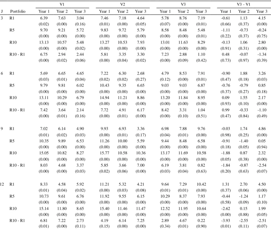
Table 6 reports the results for the longhorizon analysis of the profitability of the volume -based price momentum portfolios I am examining. This consists of annual event-time returns for three 12-month periods after the portfolio formation date, represented by the Year 1, Year 2 and Year 3 columns. Again, J is the length of the portfolio formation period. The numbers in parenthesis are simple p-values for annual returns.
Looking at the returns of the momentum portfolio (R10 – R1), we can see that price momentum profits go down significantly after the first 12 months across all volume divisio ns and for almost all formation periods, (J = 12) being the exception. For example, with a formation period of six months (J = 6), high-volume firms (V3) obtain a statistica ll y significant momentum return of 8.42 percent per year in Year 1, which goes down to 3.31 percent per year in Year 2 and then to 1.04 percent per year, that is not even statistica ll y significant, in Year 3. Unlike in Lee and Swaminathan (2000), the momentum effect is not
Table 6: Annual Event Time Returns to Volume-Based Price Momentum Portfolios
V1 V2 V3 V3 - V1
J Portfolio Year 1 Year 2 Year 3 Year 1 Year 2 Year 3 Year 1 Year 2 Year 3 Year 1 Year 2 Year 3
3 R1 6.39 7.63 3.04 7.46 7.18 4.64 5.78 8.76 7.19 -0.61 1.13 4.15 (0.02) (0.00) (0.16) (0.01) (0.00) (0.05) (0.07) (0.00) (0.01) (0.66) (0.37) (0.00) R5 9.70 9.21 5.72 9.83 9.72 5.79 8.58 8.48 5.48 -1.11 -0.73 -0.24 (0.00) (0.00) (0.00) (0.00) (0.00) (0.00) (0.00) (0.00) (0.01) (0.22) (0.37) (0.75) R10 13.13 10.57 5.48 13.27 10.53 7.93 13.01 11.63 8.29 -0.13 1.06 2.80 (0.00) (0.00) (0.02) (0.00) (0.00) (0.00) (0.00) (0.00) (0.00) (0.91) (0.31) (0.00) R10 - R1 6.75 2.94 2.44 5.81 3.35 3.30 7.23 2.88 1.10 0.48 -0.07 -1.34 (0.00) (0.02) (0.06) (0.00) (0.04) (0.02) (0.00) (0.09) (0.42) (0.73) (0.97) (0.39) 6 R1 5.69 6.65 4.65 7.22 6.30 2.68 4.79 8.53 7.91 -0.90 1.88 3.26 (0.03) (0.01) (0.04) (0.02) (0.02) (0.27) (0.12) (0.00) (0.01) (0.47) (0.18) (0.03) R5 9.79 9.81 6.02 10.43 9.35 6.65 9.03 9.03 6.87 -0.76 -0.79 0.85 (0.00) (0.00) (0.00) (0.00) (0.00) (0.00) (0.00) (0.00) (0.00) (0.37) (0.27) (0.18) R10 13.11 10.29 6.79 14.94 11.21 8.86 13.20 11.84 8.95 0.09 1.55 2.17 (0.00) (0.00) (0.00) (0.00) (0.00) (0.00) (0.00) (0.00) (0.00) (0.93) (0.10) (0.00) R10 - R1 7.42 3.64 2.14 7.72 4.91 6.17 8.42 3.31 1.04 0.99 -0.33 -1.10 (0.00) (0.01) (0.16) (0.00) (0.01) (0.00) (0.00) (0.10) (0.51) (0.47) (0.84) (0.49) 9 R1 7.02 6.14 4.90 9.93 6.93 3.36 6.98 7.88 9.76 -0.03 1.74 4.86 (0.01) (0.02) (0.03) (0.00) (0.01) (0.17) (0.04) (0.01) (0.00) (0.98) (0.25) (0.00) R5 10.35 9.89 6.53 11.26 10.00 5.59 9.44 8.48 6.58 -0.91 -1.40 0.05 (0.00) (0.00) (0.00) (0.00) (0.00) (0.00) (0.00) (0.00) (0.00) (0.18) (0.05) (0.94) R10 15.05 10.82 8.27 15.77 10.58 10.36 13.17 11.69 10.58 -1.88 0.87 2.32 (0.00) (0.00) (0.00) (0.00) (0.00) (0.00) (0.00) (0.00) (0.00) (0.05) (0.38) (0.00) R10 - R1 8.03 4.68 3.37 5.85 3.66 7.00 6.19 3.81 0.82 -1.84 -0.87 -2.54 (0.00) (0.00) (0.03) (0.02) (0.06) (0.00) (0.03) (0.04) (0.63) (0.20) (0.63) (0.07) 12 R1 8.33 4.58 5.92 11.21 5.32 4.21 9.64 7.29 10.42 1.31 2.70 4.50 (0.01) (0.04) (0.02) (0.00) (0.03) (0.08) (0.01) (0.01) (0.00) (0.37) (0.06) (0.00) R5 10.73 9.61 6.76 11.92 9.55 6.15 10.29 8.37 7.93 -0.44 -1.24 1.17 (0.00) (0.00) (0.00) (0.00) (0.00) (0.00) (0.00) (0.00) (0.00) (0.58) (0.09) (0.10) R10 15.14 11.80 8.65 15.40 11.46 11.47 12.52 11.95 10.64 -2.62 0.15 1.99 (0.00) (0.00) (0.00) (0.00) (0.00) (0.00) (0.00) (0.00) (0.00) (0.00) (0.88) (0.05) R10 - R1 6.81 7.22 2.73 4.19 6.14 7.25 2.89 4.67 0.22 -3.93 -2.55 -2.51 (0.01) (0.00) (0.11) (0.15) (0.00) (0.00) (0.34) (0.01) (0.90) (0.01) (0.11) (0.07)
always higher for high-volume firms in Year 1. We can see this in the nine-month formatio n period (J = 9), where low-volume stocks realize a momentum return of 8.03 percent per year versus 6.19 percent per year for high-volume stocks.
Based on these results, I cannot say that price momentum exhibits strong reversal after Year 1, although momentum profits do go down significantly. In fact, it would be useful to conduct an analysis with a longer horizon, namely five years, if the data were available.
Looking at the last three columns (V3 – V1), where the difference between high and low-volume stocks is reported, we observe that the results are highly insignificant. Therefore, I conclude that trading volume does not provide information about the long-term persistence of the price momentum present in my sample.
In sum, the results in Table 6 are consistent with previous research, although they differ slightly. While price momentum profits go down significantly after the first 12 months of the strategy, they do not become negative. I also document that trading volume does not predict the long-term persistence of price momentum.
4.5. Risk Adjustments
Table 7 reports the results for the time-series regressions of monthly returns of the various volume-based price momentum portfolios, in excess of the risk-free rate, on the Fama and French (1993) three factors. For the sake of simplicity, I only report the results for symmetr ic holding and formation periods of six-months (J = K = 6). The results presented extend to all other (J, K) combinations. The cells in each panel are organized as in Table 3, and they contain results for the various volume brackets (V1 through V3, and V3 – V1).
This table supports my previous findings. Firstly, none of the figures in the high minus low-volume columns (V3 – V1) are statistically significant, particularly the momentum portfolio, so there is no need to examine these results any further. Secondly, momentum profits cannot be explained by the Fama and French (1993) three-factor model.
Looking at the 𝛼 cells, that contain the estimated intercept coefficients of the regressions, we again confirm that every momentum portfolio for every volume tercile has significant l y positive alphas. For example, the alphas of the price momentum strategies, for low and high-volume stocks, are 1.17 percent and 1.07 percent, respectively, both statistically significa nt below a 0.01 percent level.
From the b cells, which contain the Beta coefficients of the portfolios, we can see that these coefficients are not very substantial in the momentum portfolios, both in magnitude and
Table 7: Risk-Adjusted Monthly Returns to Volume-Based Price Momentum Portfolios
Formation and Holding Periods : J = 6, K = 6
α b s h Portfolio V1 V2 V3 V3 - V1 V1 V2 V3 V3 - V1 V1 V2 V3 V3 - V1 V1 V2 V3 V3 - V1 R1 -0.78 -0.77 -1.10 -0.25 0.68 0.68 0.76 0.12 0.55 0.62 0.57 -0.03 0.96 0.81 0.94 -0.07 (0.00) (0.01) (0.00) (0.31) (0.00) (0.00) (0.00) (0.03) (0.00) (0.00) (0.00) (0.82) (0.00) (0.00) (0.00) (0.61) R5 0.09 0.27 -0.12 -0.23 0.63 0.56 0.68 0.00 0.44 0.39 0.29 -0.09 0.10 -0.01 0.29 0.23 (0.65) (0.19) (0.60) (0.11) (0.00) (0.00) (0.00) (1.00) (0.00) (0.00) (0.01) (0.21) (0.36) (0.92) (0.02) (0.00) R10 0.39 0.12 0.00 -0.35 0.70 0.74 0.88 0.14 0.58 0.61 0.65 0.10 -0.10 -0.14 -0.12 -0.03 (0.11) (0.64) (1.00) (0.07) (0.00) (0.00) (0.00) (0.00) (0.00) (0.00) (0.00) (0.33) (0.47) (0.37) (0.45) (0.78) R10 - R1 1.17 0.89 1.07 -0.25 0.04 0.08 0.20 0.03 0.09 0.22 0.05 -0.07 -1.04 -1.16 -1.14 0.05 (0.00) (0.01) (0.00) (0.34) (0.61) (0.31) (0.01) (0.64) (0.61) (0.22) (0.77) (0.63) (0.00) (0.00) (0.00) (0.73) Adj. R² Portfolio V1 V2 V3 V3 - V1 R1 0.75 0.71 0.74 0.02 R5 0.76 0.65 0.74 0.08 R10 0.68 0.65 0.71 0.10 R10 - R1 0.25 0.27 0.21 -0.01
statistical significance. For example, the coefficients for the market-risk premium factor are 0.04 percent for low-volume firms and 0.20 percent for high-volume firms, with p-values of 0.61 and 0.01, respectively.
Moving to the SMB and HML factors, in the s and h cells, we come to the same conclusions as in Table 3. Neither of these factors contribute to the returns of the momentum strategy. Once again, the SMB factor is seldom statistically significant and the HML loadings for the momentum portfolios are mostly negative. Additionally, there is not much differe nce between the factor loadings of high and low-volume firms. For example, the SMB loading for the momentum portfolio of high-volume companies is 0.05 percent, with a p-value of 0.77, and 0.09, with a p-value of 0.61, for the momentum portfolio of low-volume companies. The HML factor coefficient for the momentum strategies are -1.14 and -1.04 percent for high and low-volume firms, respectively, both significant below a 0.01 percent level.
Finally, the Adj. R2 cells, that contain the adjusted R2 of the regressions, tell the same
story has before. The Fama and French (1993) three-factor model cannot explain the excess returns of these price momentum strategies.
In sum, Table 7 reinforces the fact that price momentum profits go against risk-based explanations for returns, such as theories with rational markets, since they cannot be explained by the Fama and French (1993) three-factor model.
4.6. Robustness Checks
Table 8, present in the appendix, reports several robustness checks on my data sample. I test if my results only occur with the methodology used so far or if they are robust to different specifications. Namely, different portfolio partitions and for the largest 50 percent of the stocks that compose the STOXX Europe TMI.
Previously, I used a (10R, 3V) partition, which translates to 10 return portfolios and three trading volume portfolios. In this subsection I use two alternative partitions, one with three return portfolios and ten trading volume portfolios (3R, 10V), and another with five return portfolios and five trading volume portfolios (5R, 5V), whose monthly returns are reported in Panels A and B, respectively. Panel C reports the results for the largest 50 percent of the stocks in my sample. Apart from this, Table 8 is organized in the same way as Table 4. To be succinct, I only present the results for the nine-month formation period (J = 9), but the results extend to the other formation periods.
Looking at these alternative partitions, in Panels A and B, we can see that the results confirm what I have already found. Once again, I find that price momentum is only present in low-volume portfolios. For example, for a nine-month holding period (K = 9), low-volume stocks earn a monthly momentum return of 0.67 percent, for the (3R, 10V) partition, and 0.79 percent for the (5R, 5V) partition, both statistically significant at a 5 percent level. Additionally, it seems that volume differences are not significant in my sample, which can be seen in the last column of each cell. Here, none of the results are statistically significant.
Looking at the largest 50 percent of my sample of stocks, in Panel C, we can see that my previous findings still hold for this restricted sample. This proves that the price momentum returns present in my primary sample are not caused by small stocks. Like in Lee and Swaminathan (2000), momentum profits go down slightly, but they are still significant l y positive. For example, for a holding period of six months (K = 6), low-volume stocks realize a monthly return of 0.98 percent, with a p-value of 0.03.
In sum, Table 8 shows that my results are not limited to a specific partition but are robust to other specifications as well. The results are also robust to the size adjustment, meaning they are not driven by a few small stocks.
4.7. Country and Industry Adjustments
Table 9, present in the appendix, reports results for country and industry neutral volume -based price momentum strategies. For the sake of simplicity, I only present the results for the nine-month formation period (J = 9), but the results hold true for the remaining formatio n periods. Panel A contains the monthly returns for country-neutral volume-based price momentum strategies. Panel B contains the monthly returns for industry-neutral volume-based price momentum strategies. These portfolios are computed by sorting the sample of stocks by country or industry before applying the past volume and past return methodolo gy. This table is organized in the same way as Table 4.
This procedure is motivated by previous literature to ensure that my results are not driven by some unwanted effects, i.e. industry and country effects. Rouwenhorst (1998), when analyzing price momentum for the European stock market, controls for country momentum, to make sure his results are not just country specific, but general to the whole market. For example, it might be the case that if stocks from a certain country perform particularly well, the winner portfolio might be tilted towards the stocks from that country. Hence the necessity of the country neutral strategy. Moskowitz and Grinblatt (1999) find that there is significa nt
price momentum in portfolios formed by industry, or, industry momentum. So, I compute the industry neutral strategy to guarantee that my results are not caused by a specific industr y that exhibits price momentum.
Looking at Panel A from Table 9, we can see that my results are not country specific. Even though the momentum returns go down slightly from the original volume-based strategy, the previous conclusions are still valid for portfolios with diversified Western-European countries. Winners continue to consistently outperform losers, but almost only in low-volume portfolios. For example, with a nine-month holding period (K = 9), price momentum monthly returns are 0.85 percent for a low-volume portfolio of stocks, with a p-value of 0.02. When looking at the (V3 – V1) column, we can see that the results are not statistically significant. The fact that the results of the volume-based price momentum strategies are similar with and without controlling for countries, means that they are not driven by an unwanted country effect.
Turning to Panel B from Table 9, we can see that my results are also not driven by industry momentum. Again, the momentum returns go down slightly, compared to the original volume-based strategy, but the previous conclusions are still valid for portfolios with diversified industries. A price momentum strategy continues to exhibit significant positive returns, but only in the low-volume category. For example, with a six-month holding period (K = 6), price momentum monthly returns are 0.72 percent for a low-volume portfolio of stocks, with a p-value of 0.06. We can observe that high-volume stocks do not realize statistically significant price momentum profits, when controlling for industries. Finally, when looking at the (V3 – V1) column, we can see that the results are not statistica ll y significant. The fact that I first control for industries before implementing the volume-based price momentum strategy and that the results are similar to my previous findings, means that they were not driven by an unwanted industry effect.
In sum, Table 9 shows that my results are not solely explained by country or industr y effects. This proves that the price momentum anomaly comes from something other than just particular countries or industries.
4.8. Time-Series Split
Table 10, present in the appendix, reports the monthly returns for volume-based price momentum strategies for two separate time periods. Those time periods are, from January 2004 to December 2009 (Panel A) and from January 2010 to December 2014 (Panel B). To
be brief, I only present the results for the nine-month formation period (J = 9), but the results apply to the remaining formation periods. Otherwise, this table is organized as Table 4.
The purpose of this analysis is to investigate whether my results are different in the two time periods, and if so, what changed in financial markets to make that happen, and perhaps explain why trading volume loses some of its predictive power in my sample.
The results in Table 10 show that price momentum profits are only realized in the second half of my time frame, i.e. from January 2010 to December 2014. This is made clear by comparing Panels A and B of Table 10. While no price momentum portfolio exhibits significant monthly returns in Panel A, the story is much different in Panel B. For example, with a nine-month holding period (K = 9), the monthly return of a price momentum strategy of low-volume stocks is 0.36 percent, with a p-value of 0.58, in Panel A, and 1.70 percent, with a p-value of 0.01, in Panel B.
Therefore, it is clear that price momentum is only present in the most recent time period of my sample. I am led to conclude that this is due to the 2008 global financial crisis, and the turmoil it brought to capital markets. It is well known that price momentum strategies performed poorly during and shortly after this period, so it makes sense that I should obtain the results I did.
In sum, Table 10 shows that price momentum is only present in the second half of the time frame I am analyzing, i.e. from January 2010 until December 2014.
5. Discussion
In this section I discuss and interpret my main empirical results using a few different theoretical frameworks, I analyze some limitations of my own work and I explore avenues for future research.
5.1. Price Momentum Origin
In the previous section, I document that the price momentum anomaly present in my sample cannot be explained under a risk-based theory of rational markets, using time-series regressions based on the Fama and French (1993) three-factor model. I show that price momentum portfolios realize positive and significant alphas and the adjusted R2’s of these
regressions are very small.
It is important to note that my results, for a recent sample of European stocks, are substantially different from those obtained by Lee and Swaminathan (2000), for an older sample of US stocks. The main similarity in both studies is that low-volume stocks
outperform high-volume stocks. Aside from that, I do not find that high-volume portfolios command greater momentum profits nor that high-volume losers and low-volume winners exhibit more persistent price continuations. In fact, I find that only low-volume portfolios realize positive and significant price momentum profits, and that a momentum strategy that only selects low-volume stocks performs better than the simple price momentum strategy. I am led to conclude that the MLC hypothesis does not apply to my sample. Although these results do not align perfectly with the research that finds price momentum dynamics to be similar in the US and in Europe, they are reasonable, seeing as volume-based price momentum strategies have not been studied in the European market before. This disparity of results could be caused by a difference in the information content of trading volume between Europe and the US, or by a change of the said information content over time.
In light of these facts, I will now evaluate my results with the help of a few behaviora l models developed to explain the price momentum effect. These models focus on under and overreaction of stock prices, caused by boundedly rational investors.
Barberis et al. (1998) present a model where investors are affected by two types of psychological biases, that produce short-term price momentum and long-term price reversal. My results are consistent with only half of the predictions of this model, in the sense that my sample exhibits short-term price continuation but little long-term price reversal, seeing as momentum profits go down in the long-term but they do not reverse and become negative. It would be useful to conduct an analysis with a longer horizon, of up to five years beyond the portfolio formation date, if the data were available. That said, there is no obvious way to relate trading volume information to this behavioral model.
Daniel et al. (1998) propose a model where investors are generally overconfident in their ability. They suggest that this bias should be larger among stocks that are more difficult to evaluate and become more mispriced. The authors consider that stocks with low B/M ratios, or growth stocks, are harder to value. So, according to this behavioral model, growth stocks should obtain higher price momentum returns. This is consistent with my findings. Has I have mentioned, the momentum portfolios I create tend to load negatively on the HML factor. Therefore, they appear to be tilted towards growth stocks. So, the explanation for momentum returns in my sample could be that price momentum portfolios tend to invest in growth stocks that are more difficult to evaluate and become mispriced. There is still no clear role for trading volume in this behavioral model.