arXiv:1109.6806v1 [nucl-ex] 30 Sep 2011
G. Agakishiev6, A. Balanda3, D. Belver17, A.V. Belyaev6, A. Blanco2, M. B¨ohmer9, J. L. Boyard15, P. Cabanelas17, E. Castro17, J.C. Chen8, S. Chernenko6, T. Christ9, M. Destefanis10, F. Dohrmann5, A. Dybczak3, E. Epple8, L. Fabbietti8,9∗, O.V. Fateev6, P. Finocchiaro1, P. Fonte2,b, J. Friese9, I. Fr¨ohlich7, T. Galatyuk7,c, J. A. Garz´on17, R. Gernh¨auser9, C. Gilardi10, M. Golubeva12, D. Gonz´alez-D´ıazd, F. Guber12,
M. Gumberidze15, T. Heinz4, T. Hennino15, R. Holzmann4, I. Iori11,f †, A. Ivashkin12, M. Jurkovic9, B. K¨ampfer5,e, K. Kanaki5, T. Karavicheva12, I. Koenig4, W. Koenig4, B. W. Kolb4, R. Kotte5, A. Kr´asa16, F. Krizek16, R. Kr¨ucken9, H. Kuc3,14, W. K ¨uhn10, A. Kugler16, A. Kurepin12, R. Lalik8,
S. Lang4, J. S. Lange10, K. Lapidus8, T. Liu15, L. Lopes2, M. Lorenz7, L. Maier9, A. Mangiarotti2, J. Markert7, V. Metag10, B. Michalska3, J. Michel7, E. Morini`ere15, J. Mousa13, C. M ¨untz7, L. Naumann5,
J. Otwinowski3, Y. C. Pachmayer7, M. Palka4, Y. Parpottas14,13, V. Pechenov4, O. Pechenova7, J. Pietraszko7, W. Przygoda3, B. Ramstein15, A. Reshetin12, A. Rustamov7, A. Sadovsky12, P. Salabura3, A. Schmah8,a, E. Schwab4, J. Siebenson8∗, Yu.G. Sobolev16, S. Spatarog, B. Spruck10, H. Str¨obele7, J. Stroth7,4, C. Sturm4, A. Tarantola7, K. Teilab7, P. Tlusty16, M. Traxler4, R. Trebacz3, H. Tsertos13, V. Wagner16, M. Weber9, C. Wendisch5, J. W¨ustenfeld5, S. Yurevich4, Y.V. Zanevsky6
(HADES collaboration) 1
Istituto Nazionale di Fisica Nucleare - Laboratori Nazionali del Sud, 95125 Catania, Italy 2LIP-Laborat´orio de Instrumentac¸ ˜ao e F´ısica Experimental de Part´ıculas , 3004-516 Coimbra, Portugal
3Smoluchowski Institute of Physics, Jagiellonian University of Cracow, 30-059 Krak´ow, Poland 4GSI Helmholtzzentrum f¨ur Schwerionenforschung GmbH, 64291 Darmstadt, Germany 5Institut f¨ur Strahlenphysik, Helmholtz-Zentrum Dresden-Rossendorf, 01314 Dresden, Germany
6Joint Institute of Nuclear Research, 141980 Dubna, Russia
7Institut f¨ur Kernphysik, Johann Wolfgang Goethe-Universit¨at, 60438 Frankfurt, Germany 8Excellence Cluster Universe, Technische Universit¨at M¨unchen, Boltzmannstr.2, D-85748, Garching, Germany
9Physik Department E12, Technische Universit¨at M¨unchen, 85748 M¨unchen, Germany 10II.Physikalisches Institut, Justus Liebig Universit¨at Giessen, 35392 Giessen, Germany
11
Istituto Nazionale di Fisica Nucleare, Sezione di Milano, 20133 Milano, Italy 12Institute for Nuclear Research, Russian Academy of Science, 117312 Moscow, Russia
13Frederick University, 1036 Nicosia, Cyprus
14Department of Physics, University of Cyprus, 1678 Nicosia, Cyprus
15Institut de Physique Nucl´eaire (UMR 8608), CNRS/IN2P3 - Universit´e Paris Sud, F-91406 Orsay Cedex, France 16
Nuclear Physics Institute, Academy of Sciences of Czech Republic, 25068 Rez, Czech Republic 17Departamento de F´ısica de Part´ıculas, Univ. de Santiago de Compostela, 15706 Santiago de Compostela, Spain
anow at Lawrence Berkeley National Laboratory, Berkeley, USA balso at ISEC Coimbra, Coimbra, Portugal
calso at ExtreMe Matter Institute EMMI, 64291 Darmstadt, Germany dalso at Technische Univesit¨at Darmstadt, Darmstadt, Germany ealso at Technische Universit¨at Dresden, 01062 Dresden, Germany falso at Dipartimento di Fisica, Universit`a di Milano, 20133 Milano, Italy galso at Dipartimento di Fisica Generale and INFN, Universit`a di Torino, 10125 Torino, Italy
(Dated: April 29, 2013)
We present results of an exclusive measurement of the first excited state of theΣ hyperon, Σ(1385)+ , pro-duced inp + p → Σ+
+ K+
+ n at 3.5 GeV beam energy. The extracted data allow to study in detail the invariant mass distribution of the Σ(1385)+
. The mass distribution is well described by a relativistic Breit-Wigner function with a maximum atm0 = 1383.2 ± 0.9 MeV/c2
and a width of40.2 ± 2.1 MeV/c2 . The exclusive production cross-section comes out to be22.27 ± 0.89 ± 1.56+3.07
−2.10µb. Angular distributions of the Σ(1385)+
in different reference frames are found to be compatible with the hypothesis that33 % of Σ(1385)+ result from the decay of an intermediate∆++
resonance. PACS numbers: 25.75.Dw,25.75.-q
∗[email protected] ∗[email protected]
I. INTRODUCTION
The excitation spectrum of hadrons reflects proper-ties of quantum chromo dynamics (QCD) in the non-perturbative sector. Many hadrons, mesons as well as baryons, can be identified as members of multiplets
within quark models. More advanced techniques, such as various effective theories which are directly related to QCD, however, generate dynamically certain res-onances as emerging from interactions among other (more fundamental) hadrons [1]. This dual picture mo-tivates the quest for understanding the very nature of resonances or hadrons in general.
Considering theS = −1 strange baryon sector, the
Σ(1385) is the first excited state of the Σ hyperon and
has a spin of 3/2 ~ and isospin 1, in analogy to the ∆(1232) as first excited state of the nucleon. This
res-onance is characterized by a short life time that trans-lates into a natural width of35.8 ± 0.8 MeV/c2[3].
TheΣ(1385) itself is considered as a standard quark
triplet but its vicinity to theΛ(1405) in the mass
spec-trum correlates the study and understanding of the two resonances. Indeed, as pointed out in [4], within a chi-ral SU(3) lagrangian approach the anti-kaon spectchi-ral distribution is intimately related to the Λ, Λ(1405), Λ(1520), Σ and Σ(1385). In particular, the Λ(1405)
arises naturally from hadronic effective models as a mixture of aK−N and πΣ bound systems [5–7] but the contribution of the two ’molecular’ states and the dependency of theΛ(1405) formation upon the
reac-tion is still far from being understood. Any analysis of the lowest lying hyperon resonances suffers from the overlapping mass distributions, from possible interfer-ence effects through their ¯K − N coupling, and from the common decay intoΣ − π. In a first step of such an analysis we will determine theΣ(1385)+ produc-tion characteristics in theΛ − π decay channel (this paper) and addressΛ(1405) production in a
forthcom-ing publication.
The largest part of the present knowledge on the
Σ(1385) hyperon has been gained by employing
photo-production on a proton target [8] (for the cor-responding theoretical analysis cf. [9]), K−p col-lisions [10, 11], and pp colcol-lisions [12]. The latter measurement was accomplished at a beam momen-tum of 6 GeV/c corresponding to an excess energy,
defined as the energy above the production threshold,
ofǫ = 830 MeV. The HADES collaboration has
re-cently measured pp collisions at 3.5 GeV beam
en-ergy. TheΣ(1385)+is identified in theK+npπ−π+ final state via theΛπ+ decay of theΣ(1385)+(BR=
88 %), where the Λ is identified by the pπ− decay
(BR=63.9 %). The present paper reports on this
mea-surement.
Thinking of the exclusiveΣ(1385)+K+n
produc-tion in pp collisions the one-boson exchange model can be considered. In this framework several diagrams are conceivable: (i)π+,ρ+ exchange andΣ(1385)+ production in aπ+(ρ+)p − Σ(1385)+K+vertex with possible excitation of an intermediate∆++ decaying
into Σ(1385)+K+; (ii)K0(∗) exchange and
produc-tion in thepK0(∗)− Σ(1385)+vertex. Another pos-sibility is related to internal meson conversion in a
π+K+K0∗ vertex and Σ(1385)+ production in the
K0∗p − Σ(1385)+ vertex. Pion exchange diagrams
have been considered in the analysis [12], while in [13] kaon exchange has been included as well. Particularly interesting is the role of the intermediate∆++ exci-tation, as discussed in [14]. The angular distribution of theΣ(1385)+ extracted in this work provides in-formation which can serve to disentangle the different production mechanisms.
The results presented here have also to been seen in the context of a forthcoming analysis of the p(3.5 GeV)+Nb reaction, investigated with the same appa-ratus, which allows for studies of the medium modi-fications of theΣ(1385). In the nuclear medium, the Σ(1385) is predicted to suffer an attractive interaction
encoded in the real part of the self-energy resulting in
a40 MeV ”mass shift” and a broadening of the width
by a factor of two at normal nuclear matter density [15]. For further discussions of in-medium modifica-tions ofΣ(1385) see [16–18]. A first identification of
theΣ(1385) in sub-threshold heavy ion collisions has
been reported in [19], in which the statistical error of the extracted signal did not allow to draw conclusions about a possible broadening of the resonance spectral function. The measured yield of theΣ(1385) [19] is
well reproduced by a statistical model.
Baryon resonances, such as the Λ(1520) and the Σ(1385), have also triggered the interest in the
con-text of heavy ion reactions at higher energies [20, 21]. There, the measurement of the resonance abundance is thought to reflect the dynamics of their production and can be connected with a stage of the reaction prior to hadronisation [22].
Following this line of reasoning, we present here an analysis of the spectral shape of theΣ(1385)+ recon-structed in the exclusive reactionp(3.5 GeV) + p →
Σ(1385)++K++n. Our work is organized as follows.
Sections II and III present the experimental set-up to-gether with the event and particle selection. Section IV deals with techniques developed to identify the differ-ent background sources, and in section V the extracted
Σ(1385)+ signal is discussed. Sections VI and VII
deal with the differential cross section and the mod-eling of the acceptance corrections, respectively. We close with a summary and conclusions in section VIII.
II. THE EXPERIMENT
The experiment was performed with the High
Acceptance Di-Electron Spectrometer (HADES) at the
heavy-ion synchrotron SIS18 at GSI Helmholtzzen-trum f¨ur Schwerionenforschung in Darmstadt, Ger-many. HADES is a charged-particle detector con-sisting of a 6-coil toroidal magnet centered on the beam axis and six identical detection sections (with nearly complete azimuthal coverage) located between the coils and covering polar angles between 18◦ and 85◦. Each sector is equipped with a Ring-Imaging
Cherenkov (RICH) detector followed by Multi-wire Drift Chambers (MDCs), two in front of and two be-hind the magnetic field, as well as two scintillator ho-doscopes (TOF and TOFino). Lepton identification is provided mostly by the RICH and supplemented at low polar angles with Pre-Shower detectors, mounted at the back of the apparatus. Hadron identification is based on the time-of-flight and on energy-loss infor-mation from the scintillators and the MDC tracking de-tectors. In the following the TOF-TOFino-PreShower system is referred to as Multiplicity And Time-of-flight Array (META). A detailed description of the spectrometer can be found in [23].
A proton beam of∼ 107 particles/s with3.5 GeV
kinetic energy was incident on a liquid hydrogen tar-get of50 mm thickness corresponding to 0.7 %
inter-action length. The data readout was started by a first-level trigger (LVL1) requiring a charged-particle mul-tiplicity,MUL > 3, in the META system. A total of
1.14×10⁹events was recorded under these
experimen-tal conditions.
A common start time for all particles measured in one event was reconstructed as described in detail in [25]. With this method the time-of-flight information could be determined for almost all of the measured events.
III. PARTICLE IDENTIFICATION AND EVENT
SELECTION
The aim of this analysis is to reconstruct the
Σ(1385)+signal in the following reaction and decay
chain:
p(3.5GeV ) + p → Σ(1385)++ K++ n (1)
Λ + π+
p + π−.
The value of BR= ≈ 56 % accounts for the total branching ratio via this decay chain.
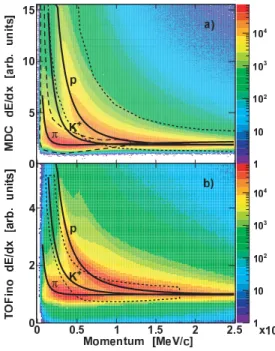
The first analysis step consists of selecting events containing four charged particles (p, π−, π+, K+). Particle identification is performed employing the en-ergy loss (dE/dx) of protons and pions in the MDCs
and adding thedE/dx information from the TOFino
system to further select kaons. The kaon selection is performed by TOFino only, because only a negligi-ble amount of kaons are observed in the TOF region. Fig. 1 shows the dE/dx distribution as a function
of the particle momentum extracted from the MDCs (panel (a)) and TOFino (panel (b)). The full black curves refer to adapted Bethe-Bloch formula [24] and the dotted and dashed lines show the cuts applied to select pion and proton candidates in the MDC: (panel (a)) and kaons in the TOFino (panel (b)). The
masses of these kaon candidates are calculated us-ing momentum and velocity. The purity of the kaon signal is then enhanced by selecting masses between
280 − 780 MeV/c2. The reconstruction of theΛ
hy-peron is achieved exploiting the decayΛ → p + π−
(BR=63.9 %). Since the Λ hyperon has a mean decay
length of cτ ≈ 7.89 cm, selections on the decay vertex can be applied to reduce the background.
The primary reaction vertex has been estimated by computing the point of closest approach between the
π+and the K+track pairs. The following topological cuts are employed to selectΛ candidates and to
en-hance the signal-to-background ratio in thep-π
invari-ant mass distribution: (1) distance between the pro-ton and pion tracks (dp−π− < 20 mm), (2) distance of closest approach to the primary vertex for the pro-ton (DCAp > 0 mm) and for the pion (DCAπ− > DCAp), (3) distance between the primary reaction ver-tex and the secondary decay verver-tex (d(Λ − V ) ≥
15 mm). The resulting invariant-mass distribution of
FIG. 1: Color online. dE/dx versus momentum for all
de-tected particles in the MDC (panel (a)) and TOFino (panel (b)) detectors. The solid black curves indicate adapted Bethe-Bloch formulas and the dashed ones show the inter-val used to select protons and pions in the MDC (panel (a)) and kaons in TOFino (panel (b)).
the selected p-π− pairs is shown in Fig. 2, in which the contribution of the Λ hyperon is clearly visible.
The background was fitted using a Landau function plus a polynomial of third order, while a Gaussian fit was applied to the signal. The obtained mean value and variance for the reconstructed mass are MΛ =
1115.2 MeV/c2andσ
Λ = 2.5 MeV/c2, respectively.
] 2 ) [MeV/c -π M(p, 1.1 1.15 1.2 1.25 3 10 × c oun ts /( 2 M e V/ c 0 1 2 3 4 3 10 × = 4206 Λ N S/B = 0.28 2 = 1115.2 MeV/c µ 2 = 2.5 MeV/c σ -π p + → Λ 2)
FIG. 2: Color online. Invariant mass distribution of selected
p-π−pairs after the K+
selection (see text for details). The two vertical lines define the mass interval select events with
Λ candidates.
events are selected for which thep-π−invariant mass is within1110 − 1120 MeV/c2(corresponding to 2.0
σ), as indicated in Fig.2by the vertical lines. A further
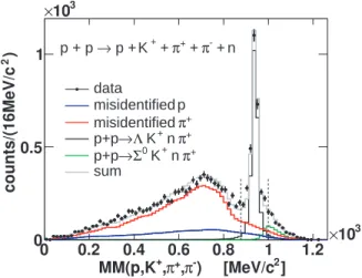
step consists in the selection of the missing neutron appearing in reaction (1), which cannot be detected in HADES. The missing mass to the four charged parti-cles (p, π−,π+, K+) is calculated after theΛ and K+ selection and the result is shown in Fig. 3. A clear
] 2 ) [MeV/c -π , + π , + MM(p,K 0 0.2 0.4 0.6 0.8 1 1.2 3 10 × 0 0.5 1 3 10 × µ data misidentified p + π misidentified + π n + K Λ → p+p + π n + K 0 Σ → p+p sum + n -π + + π + + p + K → p + p c oun ts /( 16 M e V/ c 2 )
FIG. 3: Color online. Missing mass to the four charged par-ticles p,π−,π+
and K+
, after the selection of aΛ candidate
in the same event. The gray full curve shows the sum of all identified contributions.
signal close to the nominal neutron mass is visible
(Mn = 939.5 MeV/c2, σn = 12.6 MeV/c2)
stick-ing out of a broad background distribution. Simulation studies have shown that the background to the left of the neutron peak is entirely caused by events with pro-tons and pions misidentified as kaons. The red and the
blue histograms in Fig.3show the background due to pion and proton misidentification obtained by a side-band analysis of the experimental data, as discussed in sectionIV. Additionally, Fig.3illustrates the con-tribution to the neutron signal from the non-resonant channelp + p → Λ + K++ n + π+(black histogram)
andp + p → Σ0+ K++ n + π+(green histogram).
While the shape of these two contributions is obtained by full-scale simulations, the absolute yield of these channels can be determined by fitting the total experi-mental spectrum.
Fig. 4 shows the K+ mass distribution after
the Λ selection and a cut around the neutron
mass 877 MeV/c2 < M M (p, K+, π+, π−) <
999 MeV/c2. This cut is shown by the vertical dashed
lines in Fig.3and corresponds to± 5 σ.
] 2 ) [MeV/c + Mass(K 0 0.2 0.4 0.6 0.8 1 1.2 1.4 3 10 × 0 100 200 300 + π + K p c oun ts /( 18 M e V/ c 2)
FIG. 4: Mass distribution of the selected K+
after the cuts on theΛ and missing neutron candidates (see text for details).
The vertical lines represent the nominal masses ofπ+
, K+ and proton respectively. The gray-shaded area shows the ap-plied selection on the K+mass.
IV. BACKGROUND IDENTIFICATION
Due to the incomplete purity of the kaon selection, even after all the cuts applied so far, a large fraction of the kaon candidates are still pions or protons. In particular, the contamination due to misidentified pi-ons is rather high as visible in Fig. 4. In order to estimate quantitatively this background contribution a dedicated side-band analysis based on the mass distri-bution of the selected K+candidates has been devel-oped. The goal of this analysis is to produce an event sample, which does not contain any kaon but either a pion or a proton misidentified as a kaon. To emulate the background, events have been selected containing four charged particles: one proton, one π−, one π+ and a fourth positively charged particle for which no identification is required. The mass distribution of this
fourth particle is shown in Fig.5, where one can see that most of the yield is located around the nominal pion and proton masses and that no kaon peak is visi-ble. These events represent a sample with a dominant contribution of misidentification background. A data sample with misidentified pions is explicitly extracted from the distribution in Fig. 5 by selecting the mass range of−0.25 − 0 (GeV/c2)2, while for protons the interval from0.615 to 4 (GeV/c2)2 is chosen. These background samples are analyzed in the same way as described in sectionIIIwith an exception made for the secondary vertex cuts of theΛ decay. These cuts
((1-3) in sectionIII) have been omitted in order to enhance the statistics of the background sample.
However, although the selection of the misidenti-fied pions and protons is done in a range rather distant from the nominal kaon mass, the two misidentification samples still contain a certain amount of real kaons. These real kaons are produced together with aΛ, due
-1 0 1 2 3 6 10 × 3 10 4 10 5 10 6 10 π+ + K p [(MeV/c )] 2 Mass 22 c oun ts /( 4000 (M e V/ c ) ) 2 2
FIG. 5: Count rate of all K+ candidates as a function of the squared mass. The two gray-shaded areas show the se-lectedπ+
and the protons on the left and right side, respec-tively. The dashed verticals line indicate the nominal squared masses ofπ+
, K+
and protons.
to strangeness conservation. Since the selection on the
π−-proton pairs invariant mass around theΛ nominal mass is also applied to the background samples, the contribution by real kaons is enhanced.
Our strategy to reduce the contribution of the real kaon signal to this background samples is to smear si-multaneously the momenta of the identifiedπ+andπ− such that theΛ signal in the π−-proton invariant mass distribution disappears. This way, theΛ selection in
the p-π invariant mass distribution does not enhance
the fraction of events with aK+.
A further issue to be addressed deals with the spe-cific kinematics of the particles selected via the cut around the nominal kaon mass (from here on consid-ered as fake kaons) and of the explicitely misidenti-fied pions and protons, employing the side band cut.
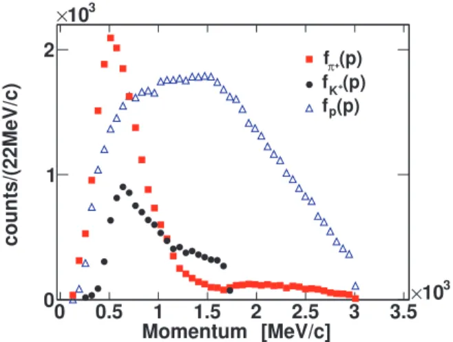
The fake kaons correspond to particles with the ’cor-rect’ kaon mass but which are not real kaons. They are contributing to the missing mass distribution shown in Fig.3mainly in the range away from the nominal neutron mass and are hence a source of background. Figure6 compares the momentum distribution of the
Momentum [MeV/c] 0 0.5 1 1.5 2 2.5 3 3.5 3 10 × c oun ts /( 22 M e V/ c ) 0 1 2 3 10 × (p) + π f (p) + K f (p) p f
FIG. 6: Color online. Momentum distribution of the fake kaons (bullets) together with the protons (triangles) and pi-ons (squares) explicitly misidentified as kapi-ons.
fake kaons (bullets) together with the momentum dis-tributions of the misidentified protons (triangles) and pions (squares). One can see that the shapes of these distributions are rather different. This difference can-not be neglected during the evaluation of background due to fake kaons, since we are performing an exclu-sive analysis with the total four-momentum being con-served.
In order to reproduce the momentum distribution of the fake kaons the following function must be determined:
γ(|~p|) = a fK+(|~p|)
π+fπ+(|~p|) + fp(|~p|)
, (2)
where fK+(|~p|), fπ+(|~p|) and fp(|~p|) are the momen-tum distributions of the fake kaons, misidentified pi-ons and protpi-ons, respectively. The factoraπ+accounts for the unknown relative contribution of the misidenti-fied pions and protons to the total background. Given a value of the parameteraπ+, each event corresponding to the pion ’side’ of the mass distribution in Fig.4is weighted by the factoraπ+ and multiplied byγ(|~p|), while each event from the proton ’side’ is weighted
withγ(|~p|) only. The total missing mass is calculated
for each weighted event and the obtained distributions are compared to the background underlying the neu-tron signal. Figure3shows the resulting missing mass generated by the two background samples (blue his-togram for protons and red hishis-togram for pions). The parameteraπ+ is varied systematically until the sum of the two background distributions gives the best fit
to the region of the spectrum on the left side of the neutron peak, i. e. for0 < M M (p, K+, π+, π−) <
870 MeV/c2. Together with the such derived
back-ground the contribution of the signal channelsp + p →
Λ + K++ n + π+andp + p → Σ0+ K++ n + π+
are displayed in Fig.3(black and green histograms re-spectively). The gray curve in Fig.3 shows the sum of all contributions, which reproduces the experimen-tal data very well. Our side-band method allows in-deed to reproduce the total background. Furthermore, the contamination by misidentified pions and protons to the signal can be evaluated quantitatively. After the cut around the nominal neutron mass in the to-tal missing mass distribution one obtains precisely the signal-to-background ratio and hence can estimate the contribution of the misidentification background to the
Σ(1385)+spectrum.
V. THE Σ(1385)+
SIGNAL
In the final step events conforming to theΛ, π+,K+ and neutron hypothesis are used to calculate theΛ-π+ invariant mass. The resulting distribution is shown in Fig.7. A clear peak at theΣ(1385)+pole mass is vis-ible on the top of some background. The contribution of the misidentification background (blue histogram) is shown together with the contributions of the direct reactions (i)p + p → Σ0+ π++ K++ n (green his-togram) and (ii)p + p → Λ + π++ K++ n (black his-togram). After the determination of the scaling factors
aπ+andγ(|~p|) the form and yield of the
misidentifica-tion background is fixed. The reacmisidentifica-tions (i) and (ii) rep-resent a source of background with the same hadrons in the final state as the reaction (1). The absolute yield of the channel (i) is determined by fitting the signal in the neutron mass spectrum shown in Fig.3, as already mentioned, while the yield of channel (ii) can only be determined by fitting the total distribution shown in Fig.7. We chose to fit the experimentalΣ(1385)+ sig-nal with a Breit-Wigner function folded with the effi-ciency and acceptance corrections thus fitting the data instead of correcting the extracted experimental signal. This method allows us also to evaluate the contribution of the background source (ii) more precisely. The used p-wave relativistic Breit-Wigner function [26] reads as follows: Breit-Wigner ∝ q 2 q2 0 m2 0Γ20 (m2 0− m2)2+ m20Γ2 , (3) Γ = Γ0m0q 3 mq3 0 F1(q), F1(q) = 1 + (q0R)2 1 + (qR)2 ,
where q is the momentum of the decay products in
theΣ(1385)+rest frame,q
0 the momentum that cor-responds to the pole mass m0, m the mass
vari-able,Γ0 the resonance width, Γ the mass-dependent width,F1(q) the Blatt-Weisskopf parameter andR =
1/197.327 MeV−1 the centrifugal barrier parameter.
Accordingly,q, q0,m, m0,Γ and Γ0are in MeV units here. The Blatt-Weisskopf centrifugal-barrier parame-ters [27] absorb possible divergences of the energy de-pendent width. In order to quantify the different contri-butions to the spectrum in Fig.7, a fit is applied to the data in the mass range1250 MeV/c2< M (Λ−π+) <
1530 MeV/c2(vertical dashed lines in Fig.7). The
to-tal fit function is composed of:
• the fixed distribution of the misidentification background and of channel (i),
• the phase-space distribution of reaction (ii) fil-tered through the geometrical acceptance and the detector efficiency scaled by one fit parame-ter and
• a corrected relativistic Breit-Wigner function with fit parameters for the mass, width and height. ] 2 ) [MeV/c + π , Λ M( 1.3 1.4 1.5 1.6 3 10 × 0 100 200 300 data non. res. Λ non. res. 0 Σ misidentification Breit-Wigner sum + π + Λ → + (1385) Σ c oun ts 2) / (8 M e V/ c
FIG. 7: Color online. Invariant mass distribution of the se-lectedΛ-π+
pairs. The circles show the experimental data, the black and green curves depict the contributions coming from the non-resonant production, the blue curve shows the misidentification background and the gray dashed curve rep-resents a Breit-Wigner distribution fitted to the data. The solid gray histogram represents the result of the final fit (see text for details). Dashed vertical lines depict the interval cho-sen for the fit.
The correction of the Breit-Wigner function is nec-essary to account for the finite available phase space and for the effects of the geometrical acceptance of the spectrometer and the efficiency of the analysis cuts that modify the measured spectral distribution in com-parison to a pure Breit-Wigner function. The geo-metrical acceptance and reconstruction efficiencies for
theΣ(1385)+have been estimated employing a
full-scale simulation. The procedure applied to extract the correct acceptance correction for the Σ(1385)+ signal is explained in detail in sections VI B. These corrections also account for the finite resolution of the apparatus which cause a broadening of theΣ(1385)+ resonance of about 3 MeV. Since the fitted
Breit-Wigner distribution is filtered through this correction, the extracted width and pole mass are already cor-rected also for the resolutions effects. In addition, the phase-space correction factor as a function of the in-variant mass must be taken into account. This
fac-1.3 1.4 1.5 1.6 3 10 × 0 100 200 300 + π + Λ → + (1385) Σ ] 2 ) [MeV/c + π , Λ M( c oun ts /( 8 M e V/ c 2) 2 MeV/c ± 0.9 =1383.2 0 m 0 Γ +0.1 -1.5 2 MeV/c ± 2.1 =40.2 +1.2-2.8
FIG. 8: Color online. Invariant mass distribution of the se-lectedΛ − π+
pairs after the background subtraction. The black circles show the experimental data together with the statistical and systematic (red squares) errors. The gray curve shows the fit with a p-wave Breit-Wigner function.
tor accounts for the loss of available phase space for the production of the neutron and K+ in the reaction
p + p → Σ(1385)+ + K+ + n with increasing
Λ-π+ invariant mass and has been evaluated via simu-lations. The product of these two corrections is folded with the Breit-Wigner distribution [26]. The product of this Breit-Wigner distribution with the correction fac-tors is shown by the gray dashed curve in Fig.7. The final result of the fit is also shown in Fig.7by the gray histogram representing the sum of all contributions. It delivers a normalizedχ2 value of about 1, a mass for
theΣ(1385)+resonance of1383.2 ± 0.9 MeV/c2and
a width ofΓ0 = 40.2 ± 2.1 MeV/c2, where the er-rors are only statistical. Also other, commonly used, parametrisations of the Breit-Wigner have been tested and they have delivered results all compatible within statistical errors The signal, after the subtraction of the three background contributions, is shown in Fig.8 to-gether with the relativistic p-wave Breit-Wigner func-tion (3) obtained by fitting the distribution shown in Fig.7. The experimental data are displayed together with the statistical and systematic errors. The system-atic errors have been evaluated modifying the analy-sis cuts as follows: the width of the cuts around the
K+, Λ and neutron missing mass have been varied
by±20 %. Additionally, the cuts applied to
recon-struct theΛ have been varied (dp−π− < 28 mm and
d(Λ −V ) ≥ 9 mm, see sectionIII). For each set of cut
values the same fitting procedure has been applied and a signal has been extracted after the background sub-traction. The obtained systematic uncertainty of the signal is shown in Fig.8by the red squares and lead to the following values for the pole mass and width of the resonance: m0 = 1383.2 ± 0.9+0.1−1.5MeV/c2
andΓ0 = 40.2 ± 2.1+1.2−2.8MeV/c2. The value of the
width is about4 MeV/c2larger than the PDG average quoted in [3]. On the other hand, the results obtained with this analysis take into account all the kinematic and efficiency effects that might modify the spectral function. The larger width of theΣ(1385)+resonance might also be due to its specific production mechanism in p+p collisions. Indeed, all the results collected in the PDG [3] refer toK−p and π+p reactions, where only a limited set ofK−p data were used to arrive to the quoted average.
Recently the CLAS collaboration published results on theΣ(1385) → Λ + γ [8] measured in photon-induced reactions; but no detailed analysis of the reso-nance mass distribution is reported upon.
VI. DIFFERENTIAL CROSS SECTIONS
The determination of the (differential) production cross sections requires extrapolation to full phase space. The corresponding (differential) acceptance corrections are obtained via a full scale simulation. Its input distributions are generated by a suitable model and tuned (iteratively) such that the model reproduces satisfactorily the obtained differential cross sections. The differential cross sections have been calculated in three reference frames which are described in the next section.
A. Reference frames and angles
The exclusive cross section in a 2 → 3 reaction with unpolarized particles, dσ/(d3pa
Ea d3p b Eb d3p c Ec ),
de-pends on four independent variables at a given value
of√s. In fact, for the reaction 1 + 2 → a + b + c,
the 9-dimensional exit phase space is constrained on a 5-dimensional hypersurface due to energy and mo-mentum conservation; azimuthal symmetry around the beam axis reduces the dimension of the exit phase space to four. Several choices of these four variables in different reference frames are conceivable [28]:
• the opposite-momentum frame in the entrance channel (p~1 = − ~p2) coinciding here with the
• an opposite momentum frame in the exit channel
(p~a= − ~pb).
In the first case, one may consider the angular distri-bution of the particlec with respect to the beam axis,
yielding aΘc
1−2 distribution. In the second case, one may consider the angular distribution of particlec with
respect to thea − b direction yielding a Θc
a−b distri-bution or with respect to particle 1 yielding a Θ1
a−b distribution.Θc
1−2is usually labeled as CMS distribu-tion of particlec, Θc
a−brefers to the helicity angle and
Θ1
a−b is the Gottfried-Jackson angle. The CMS and the Gottfried-Jackson angles connect entrance and exit channels, while the helicity angles quantify relations within the exit channel. As the selection of particle
la-belsa, b, c is arbitrary for different species, there are
three different choices for each of the angles Θc 1−2,
Θ1
a−bandΘca−b. It has to be noticed that for identical particles 1 and 2, one should averageΘ1
a−bandΘ2a−b. For different hadronsa and b we supplement the
super-script by the label of the hadron relative to which the angle is measured, e. g.,Θ1b
a−borΘ c−b a−betc.
The helicity angle distribution represents a special projection of a Dalitz plot. In particular a uniformly populated Dalitz plot results in an isotropic helicity angle distribution, whereas physical or kinematical ef-fects distorting the Dalitz plot reflect themselves in anisotropic helicity angle distributions.
The motivation for an analysis within a Gottfried-Jackson frame arises from considering e. g. the distri-bution of the angleΘΣΣ∗∗−p−K+, which is the angle of the
Σ(1385)+relative to the proton in theΣ(1385)+-K+
reference frame. This angle can give insight into the scattering process especially concerning the involved partial waves. This statement holds true also if an in-termediate resonance∆∗is excited, e.g.πp → ∆∗ →
Σ(1385)+K+.
B. Modeling of the acceptance correction
a. Angular distributions in the center-of-mass sys-tem. To extract the differential cross sections as a function of the CMS angle, the data sample was di-vided into 7 angular bins and the analysis procedure described in sections III and IV was applied. This means that for each bin the neutron missing mass spectrum was evaluated and the background was de-termined, as described in section IV. After the se-lection of the neutron, the Σ(1385)+ signal was ex-tracted from the (Λ-π+) invariant mass distribution. The misidentification background was again fixed by the fit to the neutron spectra for each of the 7 angular bins. The background contributions due to the
chan-nels p + p → Λ + K+ + n + π+ and p + p →
Σ0+ K++ n + π+were also fixed by using the
scal-ing factor from the fit to the integrated spectrum (see Fig.7). In this way the background contribution could
-1 -0.5 0 0.5 1 0 10 20 30 0.45 µb ± = 12.97 0 A 1.46 µb ± = 18.51 2 A 1.40 µb ± = 5.29 4 A /ndf = 2.01 2 χ CMS * Σ Θ cos
)
)
d σ d c o s ( Θ ) [µ b ]FIG. 9: Color online. Angular differential cross section for theΣ(1385)+
production as a function ofcos(ΘΣ∗
CM S). The
curve corresponds to a fit with a Legendre polynomials.
be subtracted, and a pureΣ(1385)+spectrum was ob-tained for each bin. Applying this binning also to the full-scale simulations, the geometrical acceptance and efficiency could be extracted in a differential form and could be used to correct the differential distributions.
The yield ofΣ(1385)+in each angular bin was ob-tained by integrating the subtracted spectra in a± 6σ interval around the pole mass, where the parameters were taken from the fit to the integrated spectrum (Fig.8). The production cross section was normalized to elastic scattering which was independently mea-sured in the same experiment [32]. Figure9exhibits the differential cross section forΣ(1385)+production as a function of the CMS scattering angle. The exper-imental data points shown in Fig.9 point to a strong anisotropy for the emission of the Σ(1385)+. This anisotropy is quantified by fitting a series of Legendre polynomials with the coefficients Ai, i= 0, 2 and 4
dσ
d cos θ = A0· L0+ A2· L2+ A4· L4, (4)
Only even polynomials are used due to the symme-try in the entrance channel. The results of the fit are listed in the legend of Fig.9. The non-zero contri-bution of the p-wave polynomialsL2 already reflects the peripheral character of the production mechanism. This differential distribution was obtained with accep-tance corrections determined by simulations in which particles are emitted according to phase space. This evaluation of the acceptance will not be sufficient if other, independent angular distributions show a devia-tion from an isotropic phase-space emission.
The angular distributions of the neutron and K+ were determined in the same way as for the§(1385). However, the interdependence of the three precludes further information about deviations from emission ac-cording to phase space.
b. Angular distributions in the helicity angle
frame. We consider now the helicity distributions
with respect to ΘΣ∗−n
n−K+, i.e. the angle between the
Σ(1385)+ and the neutron in the neutron-K+
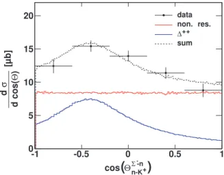
refer-ence frame. For the acceptance corrections, phase space simulations filtered by the CMS angular distri-bution of theΣ(1385)+ (see Fig.9) have been used. Since there is no obvious kinematical correlation be-tween the two anglesΘΣn−K∗−n+andΘΣ
∗
CM S, the filtering is not expected to bias the extracted distribution in the helicity frame, but accounts only for the correct accep-tance of each event. As can be seen in Fig. 10, the helicity angular distribution is not isotropic but shows a peak aroundcos(ΘΣ∗−nn−K+) = −0.5. This effect must be taken into account to get the appropriate acceptance corrections.
Higher resonances, contributing to the production of
the Σ(1385)+, could induce such an effect. In
ref. [14], the production of Σ(1385)+ for the same reaction system as analyzed in the present work,
was investigated at a beam momentum of p =
6 GeV/c. They found that a part of the Σ(1385)+
production proceeds via an intermediate ∆++ res-onance with a Breit-Wigner mass peak value of around2035 MeV/c2, followed by the decay∆++ →
Σ(1385)++ K+. The statistics was not sufficient to
-1 -0.5 0 0.5 1 0 5 10 15 20 n-K Σ -n Θ cos
(
+)
* data non. res. ∆++ sum d σ d c o s ( Θ ) [µ b ]FIG. 10: Color online. Angular differential cross section for theΣ(1385)+
production as a function ofcos(ΘΣ∗−n
nK+ ). The red and blue histograms correspond to the contributions by the non-resonant production of theΣ(1385)+
and resonant production via an intermediate∆++
, respectively.
obtain any information about the quantum numbers of this∆++ state, however, the width of the resonance was estimated to be about250 MeV. These
parame-ters were used as an input for a Monte-Carlo simula-tion of the processp + p → ∆+++ n with
subse-quent∆++decay intoΣ(1385) + K+. From the sim-ulation we obtain the shape of the angular distribution of theΣ(1385) in the helicity angle frame. Figure10
shows, together with the experimental data, simulation results stemming from non-resonant production of the
Σ(1385)+(red histogram) and via a∆++production
(blue histogram). The dashed curve shows the sum of the two simulated processes assuming a contribution
of66 % by the non-resonant production and 33 % by
the∆++ excitation. One can see that the agreement with the data is excellent. This result suggests that a rather large amount of the extracted Σ(1385)+ may be produced via an intermediate∆++ resonance. In the following it is assumed that indeed 33 % of the
reconstructedΣ(1385)+ stems from an intermediate
∆++. To obtain the appropriate filter functions for the simulations an iterative procedure is applied. In a first step the differential distribution of theΣ(1385)+
in the CMS is used to filter the non-resonant simula-tions. The differential cross section of the neutron in the CMS is used to filter the∆++simulations. This is a natural choice, as the∆++and the neutron are going back to back in this reference frame. The acceptance corrections are recalculated using the filtered simula-tion and new experimental distribusimula-tions are obtained. The process is repeated again and the new filter func-tion is extracted from the experimental distribufunc-tions.
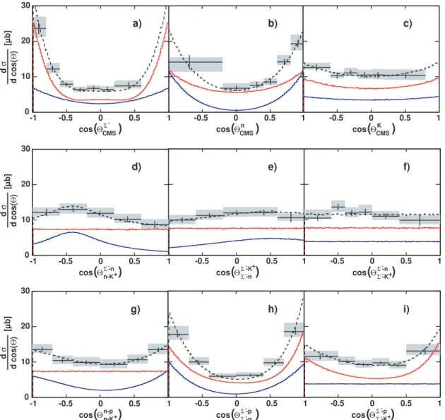
The final results after three steps of iteration are shown in Fig.11, panel (a) for theΣ(1385)+ distribu-tion in the CMS and in panel (b) for the neutron distri-bution in the CMS. In addition to the experimental data the two components of the simulated yields are drawn. The red curves represent the non-resonant contribution and the blue curve the∆++contribution. The experi-mental data are shown together with the statistical and systematic errors (gray rectangles). The systematic er-rors have been evaluated by varying the analysis cuts in the following way. The cuts on the neutron missing mass and on theΛ invariant mass have been expanded
by20 %, the cut on the K+ mass has been varied by
+20 % and −10 %. The energy loss cuts in the MDC
and TOFino detector have been also varied by±10 %. The agreement of the simulated data with the ex-perimental points in panels (a) and (b) is a constraint imposed by the iterative procedure described above, on the other hand the validity of the new acceptance correction is supported by the fact that the distribution in panel (a) is more symmetric then the one shown in Fig.9. In order to check whether the simulated model really fits to the experimental data, other, independent angular distributions have to be analyzed. Panel (c) of Fig. 11 shows the CMS angular distribution for theK+ which is also well reproduced by the simu-lated model. Panels (d), (e) and (f) depict the distri-butions of the three helicity angles and panels (g), (h) and (i) the distributions of the Gottfried-Jackson an-gles. Panel d) shows the distribution ofcos(ΘΣ∗−n
n−K+) already discussed in Fig. 10. The small differences with respect to the previous figure arise by the mod-ified acceptance correction that now takes into account the CMS angular distributions. Panel (e) represents
CMS * Σ Θ cos -1 -0.5 0 0.5 1
(
)
cos(
ΘCMS)
cos(
ΘCMS)
n K n-K n-p Θ cos -1 -0.5 0 0.5 1)
(
+ -0.5 0 0.5 1 -0.5 0 0.5 1 Σ -n Θ cos(
Σ **-p)
cos(
ΘΣ -K)
Σ -p* * + 0 10 20 30 b) c) g) h) i) n-K Σ -n Θ cos -1 -0.5 0 0.5 1)
(
+ -0.5 0 0.5 1 -0.5 0 0.5 1 Σ -n Θ cos(
Σ **-K)
cos(
ΘΣ -K)
Σ *-n * + * + d) e) f) 0 10 20 30 d) 0 10 20 30 -0.5 0 0.5 1 -0.5 0 0.5 1 a) d σ d c o s ( Θ ) [µ b ] d σ d c o s ( Θ ) [µ b ] d σ d c o s ( Θ ) [µ b ]FIG. 11: Angular differential cross sections for theΣ(1385)+
production in CMS (top row: a : ΘΣ∗
CM S, b : Θ n CM S, c : ΘK+
CM S), helicity (middle rowd : Θ Σ∗−n
n−K+, e : ΘΣ∗−K +
Σ∗−n , f : Θ
Σ∗−n
Σ∗−K+) and Gottfried-Jackson angles (bottom row: g :
Θn−p
n−K+, h : Θ
Σ∗−p
Σ∗−n, i : Θ
Σ∗−p
Σ∗−K+) angle frames. The solid curves represent the contributions by the non-resonant (blue) and resonant (red) production mechanisms, as in Fig. 10. The dashed curve shows the sum of the resonant and non-resonant contributions.
thecos(ΘΣ∗−K+
Σ∗−n ) distribution. There the anisotropy
of the experimental distribution due the∆++ contri-bution is less evident but still present. The helicity angular distribution (panel (f)) is rather flat for both the experimental and the simulated curves. A possi-ble anisotropy in the experimental data could be con-nected to the polarization of the∆++that was not in-cluded in the simulations. The data leaves some room for anisotropy but no firm conclusion can be drawn.
c. Angular distributions in the Gottfried-Jackson
frame. The experimental distributions of the
Gottfried-Jackson angles show a strong anisotropy that can be well reproduced by our simple model. The distributions shown in panels (g) and (i) of Fig. 11
are linked to the partial waves acting at the respective verteces but no specific assumption is made in our simulation. Nevertheless, these distributions are kine-matically correlated with the CMS distributions. This is also at the origin of the good agreement between the experimental and the simulated angular distributions in the helicity frame.
all kinematically independent from each other, they are here shown for the sake of completeness. These distri-butions constitute an important reference to test future theoretical models describing the production. Indeed different production mechanisms will result in differ-ent angular distributions of the decay products. It has also to be pointed out that the internal degrees of free-dom of theΣ(1385)+and the intermediate∆++ reso-nance are neglected in our simulations.
The overall agreement of the experimental data with the angular distributions modeled with the simulations justifies the usage of the resulting acceptance correc-tions, despite of the fact that the contribution by the
∆++ resonance cannot be demonstrated unambigu-ously.
C. Production cross sections
The last step of the analysis consists of the calcula-tion of the produccalcula-tion cross seccalcula-tion. The produccalcula-tion cross section has been estimated by the integration of the simulated differential cross sections adapted to the experimental data over the whole phase space for each of the nine distributions shown in Fig.11. Indeed, as-suming that proper acceptance and efficiency correc-tions have been applied, the same total cross section for the exclusive production of theΣ(1385)+resonance in the reaction pp→ n + K++ Σ+(1385) should be ob-tained.
The integration of the nine differential angular dis-tributions shown in Fig.11delivers values of the total production cross section that are in agreement within the statistical errors. The arithmetic mean of these val-ues yields22.42 ± 0.99 ± 1.57+3.04−2.23 µb. The
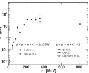
statisti-cal error is followed by a first systematic error arising from the normalization to the elastic events and a sec-ond asymmetric error stemming from the cut variations discussed above. This cross section can be compared to the values known for theΣ(1192)+ production in p+p collisions. Figure12shows the production cross sections for the reaction p + p → Σ++ K++ n as a function of the excess energyǫ. The cross section
extracted from our analysis of the channel p + p →
Σ(1385)++ K++ n is shown together with the
mea-surement at higher energies reported in [12].
The data point corresponding to the Σ(1385)+ is about a factor two lower than the cross section value extracted for the Σ+ at the same excess energy but still compatible within the systematic errors. Our data point agrees well with the value of15 ± 2 µb reported in [12] forΣ(1385)+at an excess energy of830 MeV
also in p+p collisions, pointing to a weak dependence on excess energy of bothΣ+ andΣ(1385)+ produc-tion aboveǫ = 200MeV.
[MeV] ∈ 0 200 400 600 800 [µ b ] σ -2 10 -1 10 1 10 2 10 + Σ + + n + K → p + p HIRES ANKE Sibirtsev et al. + (1385) Σ + + n + K → p + p HADES Klein et al.
FIG. 12: Color online. Production cross sections for the re-actionp + p → p + K++ Σ+
as a function of the excess energyǫ. Data points measured by several experiments have
been compiled in [33]. The production cross section for the reactionp + p → n + K++ Σ(1385)+
from this work (red star) and at6 GeV/c incident momentum [12] (blue star) are
shown as well.
VII. SUMMARY
We present the results obtained from an exclusive analysis of theΣ(1385)+ resonance produced in p+p collisions at a kinetic energy of 3.5 GeV. The sophis-ticated method developed for the reconstruction of the background allows to estimate with high precision the position and the width of this resonance. The value ex-tracted for the mass,m0= 1383.2 ± 0.9+0.1−1.5MeV/c2, agrees well with the PDG value [3], while the width,
Γ0 = 40.2 ± 2.1+1.2−2.8MeV/c2, is about 4 MeV/c2
larger than the PDG average [3].
Angular distributions have been corrected for accep-tance and detector response by means of a complete simulations testing two assumptions for the produc-tion mechanism. Our analysis suggests that a 33 %
of theΣ(1385)+ yield originates from the decay of an intermediate∆++ resonance, whereas one should underline that interference effects could also modify the kinematics of the reaction. The efficiency and acceptance corrected angular distribution of the three reference frames CM, helicity and Gottfried-Jackson have been extracted and can be used to test theoreti-cal models describing the production mechanisms for
theΣ(1385)+ state. A total production cross section
ofσ = 22.42 ± 0.99 ± 1.57+3.04−2.23 µb has been
de-duced and is found to be consistent with the systemat-ics measured for the ground stateΣ+production in the same final state as a function of the excess energy. The available data base do not exhibit a strong dependence of the production cross section on the excess energy in the range200 ≤ ǫ ≤ 800 MeV for both the ground
stateΣ+and the first excited stateΣ(1385)+. Our re-sults provide the necessary reference for further studies of the spectral shape of theΣ(1385) resonance in p+A
and A+A reactions. Furthermore, our analysis repre-sents an important bench mark for the investigation of
the Λ(1405) resonance in p+p, p+A and A+A
colli-sions. Our results will help to understand the proper-ties and production characteristics of the lowest lying hyperon resonances both in elementary and heavy ion collisions with proton induced reactions at nuclei as link between them.
Acknowledgements
The authors would like to thank Dr. B. Ketzer and Prof. W. Weise for the useful discussions. The following funding are acknowledged. LIP Coim-bra, Coimbra (Portugal): PTDC/FIS/113339/2009, SIP JUC Cracow, Cracow (Poland): NN202286038, NN202198639, HZ Dresden-Rossendorf, Dresden
(Germany): BMBF 06DR9059D, TU Muenchen,
Garching (Germany) MLL Muenchen DFG EClust: 153 VH-NG-330, BMBF 06MT9156 TP5 TP6, GSI TMKrue 1012, GSI TMFABI 1012, NPI AS CR, Rez (Czech Republic): MSMT LC07050, GAASCR IAA100480803, USC - S. de Compostela, Santiago de Compostela (Spain): CPAN:CSD2007-00042, Goethe
Univ. Frankfurt (Germany): HA216/EMMI, HIC
for FAIR (LOEWE), BMBF06FY9100I, GSI F&E01, CNRS/IN2P3 (France).
Bibliography
[1]N. Kaiser, P.B. Siegel and W. Weise, Nucl. Phys. A 594 (1995) 325;
E. Oset and A. Ramos, Nucl. Phys. A 635 (1998) 99; T. Hyodo and D. Jido, Prog. Part. Nucl. Phys. (2011), in print;arXiv:1104.4474[nucl-th].
[2]C. Hartnack, H. Oeschler, Y. Leifels, E. Bratkovskaya, J. Aichelin,arXiv:1106.2083v1.
[3]K. Nakamura et al. (PDG), J. Phys. G 37, 075021 (2010).
[4]M.F.M. Lutz, C. L. Korpa, M. Moeller, Nucl. Phys. A
808, 124 (2008).
[5] B. Borasoy, R. Nissler, W. Weise, Phys. Rev. Lett. 96 199201 (2006), Eur. Phys. J. A 25, 79. (2005); N. Kaiser, W. Weise Phys. Lett. 94, 213401 (2005).
[6] T. Hyodo, D. Jido and A. Hosaka, Phys. Rev. C 78, 025203 (2008).
[7] D. Jido, J. A. Oller, E. Oset, A. Ramos and U. G. Meiss-ner, Nucl. Phys. A 725, 181 (2003).
[8] D. Keller et al. (CLAS), Phys. Rev. D 83, 072004 (2011).
[9] Y. Oh, C. M. Ko, K. Nakayama, Phys. Rev. C 77, 045204 (2008);
Y. Oh,arXiv:1009.5789v1.
[10] M. Baubillier et al., Z. Phys. C 23, 213 (1984).
[11] M. Aguilar-Benitz, J. Salicio, Ann. Fis. A 77, 144 (1981).
[12] S. Klein et al., Phys. Rev. D 1, 3019 (1970).
[13] E. Ferrari et al., Phys. Rev 175, 2003 (1968).
[14] W. Chinowsky et al., Phys. Rev. 165, 1466 (1968).
[15] M. Kaskulov, E. Oset, Phys. Rev. C 73, 045213 (2006).
[16] W. Cassing, L. Tolos, E. L. Bratkovskaya, A. Ramos, Nucl. Phys. A 727, 59 (2003).
[17] J. Schaffner-Bielich, V. Koch, M. Effenberger, Nucl. Phys. A 669, 153 (2000).
[18] M. F. M. Lutz, Prog. Part. Nucl. Phys. 53, 125 (2004).
[19] X. Lopez et al. (FOPI), Phys. Rev. C 76, 052203 (2007).
[20] B. I. Abelev et al. (STAR), Phys. Rev. C 78, 044906 (2008).
[21] C. Markert et al. (STAR), J. Phys. G 35, 044029 (2008). I. Kuznetsova, J. Rafelski, Phys. Rev. C 79, 014903 (2009).
[22] S. Vogel, J. Aichelin, M. Bleicher, J. Phys. G 37, 094046 (2010).
[23] G. Agakichiev et al. (HADES), Eur. Phys. J. A 41, 243 (2009).
[24] A. Schmah, doctoral thesis, Darmstadt (2008);
http://www.gsi.de/documents/DOC-2008-May-84-1.pdf [25] J. Siebenson, Master Thesis,
Tech-nische Universit¨at M¨unchen, 2010;
http://www.gsi.de/documents/DOC-2011-Jan-46.html [26] J. D. Jackson, Nuovo Cimento 34, 1644 (1964).
[27] F. von Hippel, C. Quigg, Phys. Rev. 5, 624 (1972).
[28] M. Abdel-Bary et al. (COSY-TOF) Eur. Phys. J. A 46, 27 (2010).
[29] I. Zychor et al. (ANKE), Phys. Lett. B 660, 167 (2008).
[30] K. Bockmann et al. (Bonn-Hamburg-Munich), Nucl. Phys. B 143, 395 (1978).
[31] S. R. Borenstein et al., Phys. Rev. D 9, 3006 (1974).
[32] R. C. Kammerud et al., Phys. Rev. D 4, 5 (1971).