Impact of chromossomal structure on the evolution of Schizosaccharomyces pombe undergoing Mutation Accumulation

(1)

Gustavo Nuno Martins Eduardo

Licenciado

Impact of chromossomal structure on the

evolution of Schizosaccharomyces

pombe undergoing Mutation

Accumulation

Dissertação para obtenção do Grau de Mestre em Genética Molecular e Biomedicina

Orientador: Lília Perfeito, PhD, Principal Investigator no

Instituto Gulbenkian de Ciência.

Júri:

Presidente: Prof. Doutora Paula Gonçalves Arguente: Prof. Doutor Francisco Dionísio

Vogal: Prof. Doutora Lília Perfeito

(2)

Outubro, 2015

LOMBADA

Impac t o f ch ro moss om al s tructu re on t he ev olut ion of S ch izos ac ch a romy ce s po mbe und ergo ing M u tati on A cc umulat ion

(3)

Department of Life Sciences, Faculty of Sciences and Technology, New University of Lisbon Evolution and Genome Structure Group, Instituto Gulbenkian de Ciência

Gustavo Nuno Martins Eduardo

Impact of chromossomal structure on the evolution of

Schizosaccharomyces pombe undergoing Mutation Accumulation

Dissertation to obtain an MSc in Molecular Genetics and Biomedicine

(4)

October 2015

Impact of chromossomal structure on the evolution of Schizosaccharomyces pombe undergoing Mutation Accumulation

Copyright Gustavo Nuno Martins Eduardo, FCT/UNL, UNL

A Faculdade de Ciências e Tecnologia e a Universidade Nova de Lisboa têm o direito, perpétuo e sem limites geográficos, de arquivar e publicar esta dissertação através de exemplares impressos reproduzidos em papel ou de forma digital, ou por qualquer outro meio conhecido ou que venha a ser inventado, e de a divulgar através de repositórios científicos e de admitir a sua cópia e distribuição com objectivos educacionais ou de investigação, não comerciais, desde que seja dado crédito ao autor e editor.

(5)

Aknowledgements

To my parents. Another step on the ladder.

I’d like give Lília Perfeito my most profound gratitude. I can’t thank you enough for this opportunity. Thank you for all I’ve learned while working in the EGS group and for all the help you’ve given me during this past year.

This thank you extends to all the people I’ve worked with in my time here. Catarina, Diogo, Paula, Sara, Simone, this Thesis wouldn’t have been done without you. I include here Isabel Gordo, for giving me ideas I would not have thought of otherwise. And, of course, to Teresa Avelar, who has never met me but without whose work mine would not have been possible. And I could not forget Rui Gardner, Cláudia and Cláudia, for all the help they gave me with the FACS technique.

I’d also like to thank Prof. Paula Gonçalves, for being understanding of my situation and helping me when I most needed it.

Thanks to all the MIGS, to Mauro and to Lucas for the support and for trying to keep me socially active.

(6)

i

LIST OF FIGURES

Figure 1.1: Graphical representation of the chromosomes and chromosomal rearrangements present in the strains used during this project. ... 5 Figure 2.1 Example of YES agar plate used to streak each strain’s 12 cell lines. The grid pattern allows us to streak all 12 on the same plate, one per area. ... 9 Figure 2.2 LSR Fortessa interface, showing an example of a well’s cells being separated through the three windows and between the mCherry-marked reference competitor and the interest sample strain. ... 13 Figure 3.1: Probability of isolating one, two or three cells per bottleneck. The error bars represent standard deviation from the mean. The data represents the pooled results of three experiments, each analyzing 96 streaks ... 19 Figure 3.2 Average fitness trajectories for strains SPP26 (in light blue) and SPP27 (in dark blue) across three different bottleneck numbers: B0, B48 and B144. For B0 the error bars represent experimental error from several measurements of the ancestral strain, while for B48 and B144 they represent the variance between all 12 cell lines per strain. * shows a significant change in fitness distributions between both bottleneck numbers, while Δ does the same for fitness average. */Δ p-value < 0.05; **/Δ Δ p-value < 0.01; ***/Δ Δ Δ p-value < 0.001. Bonferroni corrections were applied to all p-values. ... 21 Figure 3.3 Average fitness trajectories for strains C2 (blue) and I2 (red) across three different bottleneck numbers: B0, B48 and B144. For B0 the error bars represent experimental error from several measurements of the ancestral strain, while for B48 and B144 they represent the variance between all 12 cell lines per strain. * shows a significant change in fitness distributions between both bottleneck numbers, while Δ does the same for fitness average. */Δ p-value < 0.05; **/Δ Δ p-value < 0.01; ***/Δ Δ Δ p-value < 0.001. Bonferroni corrections were applied to all p-values. ... 22 Figure 3.4 Average fitness trajectories for strains C4 (blue) and T4 (red) across three different bottleneck numbers: B0, B48 and B144. For B0 the error bars represent experimental error from several measurements of the ancestral strain, while for B48 and B144 they represent the variance between all 12 cell lines per strain. * shows a significant change in fitness distributions between both bottleneck numbers, while Δ does the same for fitness average. */Δ p-value < 0.05; **/Δ Δ p-value < 0.01; ***/Δ Δ Δ p-value < 0.001. Bonferroni corrections were applied to all p-values. ... 23 Figure 3.5 Average fitness trajectories for strains C5 (blue), T5 (red) and SPP20 (pink) across three different bottleneck numbers: B0, B48 and B144 (not performed for SPP20 at this time). For B0 the error bars represent experimental error from several measurements of the ancestral strain, while for B48 and B144 they represent the variance between all 12 cell lines per strain. * shows a significant change in fitness distributions between both bottleneck numbers, while Δ does the same for fitness average. */Δ

(9)

iv p-value < 0.05; **/Δ Δ p-value < 0.01; ***/Δ Δ Δ p-value < 0.001. Bonferroni corrections were applied to all p-values. ... 24 Figure 3.6 Average fitness trajectories for strains C8 (blue) and T8 (red) across three different bottleneck numbers: B0, B48 and B144. For B0 the error bars represent experimental error from several measurements of the ancestral strain, while for B48 and B144 they represent the variance between all 12 cell lines per strain. * shows a significant change in fitness distributions between both bottleneck numbers, while Δ does the same for fitness average. */Δ p-value < 0.05; **/Δ Δ p-value < 0.01; ***/Δ Δ Δ p-value < 0.001. Bonferroni corrections were applied to all p-values. ... 25 Figure 3.7 Average fitness trajectories for strains C10 (blue) and T10 (red) across three different bottleneck numbers: B0, B48 and B144. For B0 the error bars represent experimental error from several measurements of the ancestral strain, while for B48 and B144 they represent the variance between all 12 cell lines per strain. * shows a significant change in fitness distributions between both bottleneck numbers, while Δ does the same for fitness average. */Δ p-value < 0.05; **/Δ Δ p-value < 0.01; ***/Δ Δ Δ p-value < 0.001. Bonferroni corrections were applied to all p-values. ... 26 Figure 3.8 Change in variance from B0 to B144 for each individual strain, with the exception of SPP20, which shows the difference in variance between B0 and B48. ... 27 Figure 3.9 Relationship between initial fitness (B0) and average fitness at B144. ... 30 Figure 3.10 Relationship between initial fitness (B0) and average fitness at B144 for strains SPP26, I2, C2, C4, T5, C5, T8, C8, T10 and C10. ... 30 Figure 3.11 Distribution of fitness frequencies of 2 sets of hybrids: those resulting from a cross between ancestral C5 and ancestral C4 strains (green line); and those resulting from the cross between ancestral C5 and a C4 line that underwent 48 bottlenecks (purple line). ... 32 Figure 3.12 Distribution of fitness frequencies of two sets of hybrids: those resulting from a cross between ancestral C5 and ancestral T4 strains (green line); and those resulting from the cross between ancestral C5 and a T4B48 strain (purple line). ... 33

(10)

v

LIST OF TABLES

Table 2.1 Strains used in this Thesis. ... 8 Table 3.1 Results from fitting the Analysis of Variance Model (ANOVA) comparing ∆W (fitness at B144 subtracted from fitness at B0) all lines from different genomic backgrounds. Red indicates p-value < 0.05, yellow indicates 0.01 > p-value > 0.001 and green indicates 0.001 > p-value. Bonferroni corrections were applied to all p-values. ... 27 Table 3.2 Fitness decline per mutation, arising mutations per generation, associated errors and mean mutation per generation of each strain. ... 29 Table 3.3 Results of the fit of a 3-Way ANOVA correlating the presence of each auxotrophic marker in C5/C4.3 hybrid samples with those samples’ fitness level as the dependent variable. * p-value < 0.05; ** p-value < 0.01; *** p-value < 0.001 ... 34 Table 3.4 Results of the fit of a 3-Way ANOVA correlating the presence of each auxotrophic marker in C5/T4.11 hybrid samples with those samples’ fitness level as the dependent variable. * p-value < 0.05; ** p-value < 0.01; *** p-value < 0.001 ... 35 Table 6.1 C5+C4.3 and C5+T4.11 samples organized by tetrad the spore originated from and marked with parental or mixed phenotypes. ... 47 Table 6.2 Individual fitness values for all replicates of strain SPP26 and corresponding lines, across bottlenecks 0, 48 and 144. Blank cells represent replicates that could not be measured or were used as controls. ... 48 Table 6.3 Individual fitness values for all replicates of strain SPP27 and corresponding lines, across bottlenecks 0, 48 and 144. Blank cells represent replicates that could not be measured or were used as controls. ... 49 Table 6.4 Individual fitness values for all replicates of strain I2 and corresponding lines, across bottlenecks 0, 48 and 144. Blank cells represent replicates that could not be measured or were used as controls. ... 50 Table 6.5 Individual fitness values for all replicates of strain C2 and corresponding lines, across bottlenecks 0, 48 and 144. Blank cells represent replicates that could not be measured or were used as controls. ... 51 Table 6.6 Individual fitness values for all replicates of strain T4 and corresponding lines, across bottlenecks 0, 48 and 144. Blank cells represent replicates that could not be measured or were used as controls. ... 52 Table 6.7 Individual fitness values for all replicates of strain C4 and corresponding lines, across bottlenecks 0, 48 and 144. Blank cells represent replicates that could not be measured or were used as controls. ... 53

(11)

vi Table 6.8 Individual fitness values for all replicates of strain T5 and corresponding lines, across bottlenecks 0, 48 and 144. Blank cells represent replicates that could not be measured or were used as controls. ... 54 Table 6.9 Individual fitness values for all replicates of strain C5 and corresponding lines, across bottlenecks 0, 48 and 144. Blank cells represent replicates that could not be measured or were used as controls. ... 55 Table 6.10 Individual fitness values for all replicates of strain SPP20 and corresponding lines, across bottlenecks 0, 48 and 144. Blank cells represent replicates that could not be measured or were used as controls. ... 56 Table 6.11 Individual fitness values for all replicates of strain T8 and corresponding lines, across bottlenecks 0, 48 and 144. Blank cells represent replicates that could not be measured or were used as controls. ... 57 Table 6.12 Individual fitness values for all replicates of strain C8 and corresponding lines, across bottlenecks 0, 48 and 144. Blank cells represent replicates that could not be measured or were used as controls. ... 58 Table 6.13 Individual fitness values for all replicates of strain T10 and corresponding lines, across bottlenecks 0, 48 and 144. Blank cells represent replicates that could not be measured or were used as controls. ... 59 Table 6.14 Individual fitness values for all replicates of strain C10 and corresponding lines, across bottlenecks 0, 48 and 144. Blank cells represent replicates that could not be measured or were used as controls. ... 60 Table 6.15 Individual fitness values for all replicates of the recombinant hybrids ... 61

(12)

vii

Abbreviations 96 Deep Well plate – VWR 96-well deep well blocks

96 small well plate – Corning Incorporated COSTAR 96 Well Cell Culture Plates B0 – Ancestral cell line

B48 – Cell line after 48 bottlenecks B144 – Cell line after 144 bottlenecks ºC – Degrees Celsius

C – Control strain

FACS – Fluorescence Activated Cell Sorting

FM – Freezing Medium

I – Strain carrying a chromossomal inversion KS test – Kolmogorov-Smirnov test

MA – Mutation Accumulation

MCMC – Markov Chain Monte-Carlo mL – Mililiters

nm – Nanometer

PMG – Pombe Glutamate Medium RPM – Rotations Per Minute.

T – Strain carrying a chromosomal translocation Wilcox test – Mann-Whitney-Wilcoxon test WT – Wild Type strain

YES – Yeast Extract with Supplements

Ud – Mean number or arising deleterious mutations per generation

sd – Fitness decline caused by each deleterious mutation (selection coefficient)

(13)

viii sd – Error associated with sd

Ud – Error associated with Ud

∆W – Change in fitness (fitness at bottleneck 144 subtracted from ancestral fitness)

µL – Microliters

(14)

ix

Abstract

Large chromosomal rearrangements are common in natural populations and thought to be involved in speciation events. In this project, we used experimental evolution to determine how the speed of evolution and the type of accumulated mutations depend on the ancestral chromosomal structure and genotype. We utilized two Wild Type strains and a set of genetically engineered Schizosaccharomyces pombe strains, different solely in the presence of a certain type of chromosomal variant (inversions or translocations), along with respective controls. Previous research has shown that these chromosomal variants have different fitness levels in several environments, probably due to changes in the gene expression along the genome. These strains were propagated in the laboratory at very low population sizes, in which we expect natural selection to be less efficient at purging deleterious mutations. We then measured these strains’ changes in fitness throughout this accumulation of deleterious mutations, comparing the evolutionary trajectories in the different rearrangements to understand if the chromosomal structure affected the speed of evolution. We also tested these mutations for possible epistatic effects and estimated their parameters: the number of arising deleterious mutations per generation (Ud) and each one’s mean effect (sd).

Resumo

Grandes rearranjos cromossómicos são comuns em populações naturais e crê-se que estejam envolvidos em eventos de especiação. Neste projecto, usámos evolução experimental para determinar em que medida o ritmo da evolução e o tipo de mutações acumuladas dependem da estrutura cromossómica ancestral e do genótipo. Utilizámos duas estirpes Wild Type e um conjunto de estirpes de Schizosaccharomyces pombe geneticamente alteradas, juntamente com os respectivos controlos. Investigação prévia demonstrou que estas variantes cromossómicas apresentam diferentes níveis de fitness em vários ambientes, provavelmente devido a à alteração da expressão génica ao longo do genoma. Estas estirpes foram propagadas no laboratório com tamanhos populacionais diminutos, que nós expectamos que levem a selecção natural a não ser tão eficiente a eliminar mutações deletérias. Medimos as alterações de fitness destas estirpes ao longa da acumulação de mutações deletérias, comparando as trajectórias evolutivas dos diferentes rearranjos para entender se a estrutura cromossómica afecta o ritmo da evolução. Também testámos os possíveis efeitos epistáticos destas mutações e estimámos os seus parâmetros: o número de mutações deletérias que surgem por geração (Ud) e o efeito médio de cada uma (sd).

Keywords: Schizosaccharomyces pombe; Chromosomal rearrangements; Mutation Accumulation;

(15)

1

1. Introduction

1.1 State of the art and objectives

The study of evolution has come a long way since its inception. Our understanding of our biology and how life came to be was revolutionized with Darwin’s ideas on the origins of species (Darwin 1859), which introduced terms such as evolution and natural selection into popular parlance. Darwin’s discoveries spurred many doubts, and breached just as many taboos, on when and how Life itself had come to be (Dunwell, 2007). One concept that would later strengthen Darwin’s hypothesis was the existence of genes. The study of heredity, and by consequence genetics, was first pioneered by Mendel in 1865 through the study of peas. Perhaps due to such humble beginnings, his discoveries would be forgotten for over three decades until de Vries and others once more found Mendel’s manuscripts and published his findings. Despite that world-changing insight into the very nature of life itself, it would not be until 1906 that Bateson would try, on an address aimed at the Neurological Society of London, to convince the members of the Society to consider the importance the study of heredity and genetics had on the human condition (Bateson, 2009). With time, this fledgling area of Science grew in size and importance. In one century, the field of Genetics has grown from applied horticulture to a branch of Science that integrates plant, animal, microorganical, fungal and human research. With today's knowledge of DNA and RNA, epigenetics and inheritance, the study of genetics and evolution has proven its importance as a useful tool in the realms of not only horticulture, but also animal husbandry, oncology and pharmacology, among many others (Dunwell, 2007).

And yet, despite all of these advances, we still can’t fully answer the question: How does evolution work? Evolutionary biologists have struggled for decades to provide a definitive answer. Although the general mechanisms through which evolution works are well known, including natural selection, random mutations and recombination, there are still many factors that cloud our understanding of this process so necessary for the existence of life on Earth. For example, what are the advantages and disadvantages of sexual reproduction when compared to asexuality (Morran et al., 2009). Or what is the exact relationship between selection and mutation, the balance of which maintains standing genetic variance (Barton, 2010).

Since mutation is the ultimate source of all genetic variation (Barton, 2010), studies of the accumulation of deleterious mutations under controlled selection environments can shed light on several topics related to evolution and its workings (Chevin, 2011; Gordo & Dionisio, 2005)

With that in mind, we performed a Mutation Accumulation (MA) experiment. MA consists in reducing the population size and hence increasing the role of genetic drift in an evolving population. It leads to the random accumulation of mutations, independently of their effects on fitness. It was first pioneered

(16)

2 in Drosophila melanogaster (Bateman, 1959) and later adapted to different organisms, including Saccharomyces cerevisiae (Zeyl & DeVisser, 2001) and Escherichia coli (Kibota & Lynch, 1996). More recently, it was used in combination with whole genome sequencing to estimate the base substitution rate in Schizosaccharomyces pombe (Farlow et al., 2015).

MA experiments allow us to address whether different strains accumulate deleterious mutations at different rates or in different ways (in opposition, and complementation, of an adaptation experiment). In order to do that, first we must decrease selective pressure to its absolute minimum, so any mutation that’s accumulated can be carried on to the descendants. Since we can only propagate survivors, this experimental design cannot capture lethal mutations.

S. pombe growing in asexual conditions propagates by binary fission, such that two sister cells are produced with the exact same genotype with the exception of new mutations. As they grow, they will naturally compete for space and nutrients present in their environment, so even if mutations have small effects, the one that allows its carrier cell to be fitter will be selected for. In an MA, we want to reduce this competition as much as possible. The way to do this is to isolate a single cell, so all of its descendants will carry its own accumulated mutations without competing with other, fitter genotypes. Such precautions, along with usual microbiological research staples such as growing the cells at optimal growth temperatures and consistently applying the same treatments to all our cultures, allow us to ensure the carry-over of mutations, even those with highly deleterious effects, over thousands of generations. We use rich media so all genotypes have the same advantage when it comes to gathering nutrients from the medium; for example, if a cell mutates in a way that it can no longer produce a certain aminoacid it needs, it will die in a medium without that aminoacid. Hence, the mutations responsible for that inability to produce the aminoacid will be selected against.

Unlike previous studies, we performed this experiment using strain with several chromosomal rearrangements of Schizosaccharomyces pombe (S. pombe). It has been estimated that three quarters of all species of Drosophila are polymorphic for inversions, and chromosomal rearrangements are common in natural isolates of S. pombe. It might be the case that chromosomal rearrangements contribute to the processes of speciation and adaptation (Avelar, 2012). If so, then we expect different chromossomal rearrangements to take different trajectories throughout their evolution, even if the same genetic material is present in all of them. The fact that the genome has been reorganized may lead to the appearance of different mutations, or similar mutations that have differing effects.

In another area of investigation, the dynamics between epistasis and evolution still pose several questions which are not fully understood (de Visser et al., 2011). Epistasis is a phenomenon whereby the combined effect of two mutations is different from simply adding the effects of the mutations in isolation. Since an MA produces lines with large numbers of mutations, it is an ideal raw material to study epistasis. For that effect, we crossed mutated strains with a non-mutated background. In order to

(17)

3 control for genetic background effects, we also crossed non-mutated versions of those same strains with the same non-mutated background. As such, the difference between the recombinant spores produced from those crosses should be exclusively due to the presence of the accumulated mutations.

To analyze these crosses we dissected the tetrads formed from each cross, separating their individual recombinant spores. This technique gives us great statistic power, as it allows us to peer into what’s happening within each of the four spores each tetrad carries, instead of averaging out their genotypes.

In short, we began this work with the intention to answer three main questions:

1. Will chromosomal rearrangements alter the accumulation of mutations and/or their effects? 2. Are the accumulated mutations epistatic in effect?

3. How do our strains’ mutation parameters compare to those estimated for other species?

1.2 On S. pombe

S. pombe was the model organism chosen for our work due to, firstly, the common advantages it shares with other microbiological models, such as that it is easy to grow and store in large numbers. It is also easy to genetically manipulate, useful traits when studying adaptation and evolution (Avelar et al., 2013). We have extensive knowledge of its biology, particularly when it comes to chromosome maintenance. It is therefore an ideal model to study the interplay between genome architecture and evolution.

S. pombe is also preferentially haploid; in a study done by Brown et al., out of 81 natural isolate and 3 laboratory strains, only 1 was diploid (Brown et al., 2011). The strains we use in our lab are all haploid as well, entering a temporary state of diploidy only if reproducing sexually (Avelar, 2012) . Haploidy ensures that any given mutation’s effect on phenotype will be expressed without any homologous alleles to mask its expression.

Being an eukaryotic organism, the findings on S. pombe might later be applicable to other eukaryotic genomes, including humans. Its genome has also been fully sequenced. Most of these characteristics are shared by other organisms, such as Saccharomyces cerevisiae. We chose to study S. pombe for its lower number of chromosomes, which are larger in size than in S. cerevisiae. In such a genome, there are less possible combinations of chromosomal rearrangements and each has a bigger effect, since it affects more genes. It also has the distinction of being the eukaryote with the lowest number of genes, lower even than some prokaryotes (Yanagida, 2002).

(18)

4

1.3 On our genomic alterations

Besides strains carrying chromosomal rearrangements and their respective controls, we also used two Wild Type-like strains in our experiments, SPP26 and SPP27, which were isolated from a natural strain and propagated in labs before being donated to our collection. SPP26 was donated to us from the Portuguese Yeast Culture Collection at Faculdade de Ciências e Tecnologia (FCT) by Dr. José Paulo Sampaio. SPP27 was descended from Urs Leopold’s original natural isolates and was donated to us by the I. Tolic in Gottingen, Germany.

For our chromossomal rearrangement-carrying strains, we used those engineered by Teresa Avelar during her PhD Thesis Project “Chromosomal structure: a selectable trait for evolution”. We used 10 strains engineered by her: 5 rearrangements (4 translocations and 1 inversion) and 5 controls. Inversion 2 (I2) is an inversion in chromosome 2, between the sites of the arg7 and lys4 genes. Translocation 4 (T4) has translocated parts of the long arms of chromosomes 2 and 3. Translocation 5 has translocated parts of the short arm of chromosome 1 and the long arm of chromosome 2. Translocation 8 (T8) has translocated parts of the short arm of chromosome 2 and the long arm of chromosome 3. Translocation 10 (T10) has translocated parts of the short arm of chromosome 1 and the long arm of chromosome 3. These were created using the Cre–loxP system, in which a gene disruption cassette is ﬂanked by loxP sites (Avelar, 2012). The insertion of these loxP cassettes in specific locations of the chromosomes allows chromosomal breakage and following recombination between those locations (Avelar, 2012; Carter & Delneri, 2010). Each of these rearrangements has a corresponding control strain: Inversion 2 corresponds to Control 2 (C2), Translocation 4 to Control 4 (C4), etc. These control strains carry the same genotype as the parental strain, except for with the addition of the loxP cassettes in the same locations as its respective rearrangement strain, which are inserted without causing the subsequent breakage and chromosomal rearrangement. Graphical representations of their chromosomes can be seen in Figure 1.1.

All strains used in this project were of the h- mating type with the exception of C5, which is h+. Later on in the experiment we added another strain, SPP20, which is an h- variation of C5, to control for this fact.

(19)

5

Figure 1.1: Graphical representation of the chromosomes and chromosomal rearrangements present in the strains used during this project. The different colors indicate the parental chromosome of origin of each DNA stretch. The arrow shows an inversion. Figure adapted from Avelar 2013.

As such, all chromosomal rearrangements and all their respective controls have the same genetic material, with the exception of their auxotrophic markers. The only difference between them is the organization of this material within the genome.

1.4 Recombination and genetic interactions

Using S. pombe as a model organism has one distinct advantage: we can control its sexual and asexual reproductive cycles. Most S. pombe grown in laboratories throughout the world have two mating types, h+ and h-. One mating type can only sexually reproduce with the other, never with its own mating type. A cell’s mating type is determined by the allele present in the mat1 locus: mat1-P for h+ and mat1-M for h-. In the wild, S. pombe actually tends to be of the h90_{mating type. These are cells that can freely}

interchange between the two mating types (so called because 90% of the cells in a culture are capable of switching). These are converted to either h+ or h- cells through the silencing of the opposite mating type’s gene (Forsburg & Rhind, 2006).

As stated before, with the exception of strain C5, all strains used in this project were of the h- mating type.

Merely being in the presence of the opposite mating type is not enough for sexual reproduction to occur. If in rich medium, S. pombe will opt to reproduce asexually, for maximum daughter-cell production. If

(20)

6 starved of nitrogen, however, it will instead opt to produce meiotic spores (Forsburg & Rhind, 2006). This allows us to choose when and what strains will reproduce sexually, and allows us to keep all others reproducing asexually throughout our experiments.

(21)

7

2. Materials and Methods

2.1 Material, media and strains

We grew S. pombe in three different media, depending on the experiment. As rich medium we used Yeast Extract plus Supplements (YES) medium, in both solid and liquid forms. Liquid YES is composed of Yes Extract and glucose, supplemented with adenine, histidine, leucine, uracil and lysine. Solid plates are made with YES agar, which follows the same recipe with the addition of 20g/L agar. As minimal medium we used Pombe Glutamate Medium (PMG), composed of potassium hydrogen phthalate, Na2HPO4 and supplemented with salt, mineral and vitamin stocks. PMG without a carbon source was

used to incubate cells in order to increase expression of the fluorescent protein mCherry. This medium allows us to keep S. pombe alive in solution for up to 48 hours at 4ºC with no change in cellular frequencies, either by growth or by cell death. Strains were crossed on Malt Extract medium (mating medium), composed of Bacto-malt extract supplemented with arginine and lysine. Selective media were based on PMG-Glucose agar, adapting the recipe for the removal of one aminoacid at a time for each. All recipes were adapted from “Basic methods for fission yeast”(Forsburg & Rhind, 2006):

All pipetting, streaking and unfreezing procedures were done in sterile conditions using a Bunsen burner. To aid in avoiding possible bacterial contaminations, all media was supplemented with 0.1 µg/mL ampicillin.

Liquid cultures were grown in VWR 96-well deep well blocks (from here on out referred to as 96 Deep Well plate). These plates can hold up to 2 mL of volume. The high number of wells allows us to grow several strains at once or to do a high number of replicates for each experiment, as well as allowing us to discount wells for blanks and controls and still keep most wells producing data for later analysis. Corning Incorporated COSTAR 96 Well Cell Culture Plates (from here on out referred to as 96 small well plate) can carry up to 200µL of volume and they were used for two purposes: to hold samples to be frozen at -80ºC, their small size allowing us to store a large number of samples in a limited space; and for samples to be read in LSR Fortessa equipment, as mentioned on pages 20 and 21. The high number of wells gives us the same advantages mentioned for 96 Deep Well plates, and since both types of plate have the same number of wells, it is easy to pipette samples from one type of plate to the corresponding well on the other type, so we are sure of what’s in each well throughout a whole experiment.

The strains used in this Thesis had previously been created and described in “Chromossomal structure: a selectable trait for evolution” (Avelar, 2012), and are described in Table 2.1.

(22)

8

Table 2.1 Strains used in this Thesis.

Code Genotype Common name Creator

SPP26 PYCC 4197 matM:nat Wild Type PYCC4197

SPP27 L972 matM:nat Wild Type L972

C2 h- arg7::padh1-loxP- kanMX6R lys4::loxP-ura4- kanMX6R mat1-M::mat1-M-natMX6 leu1-32 ade6-M216

ura4+

Control 2 Teresa

Avelar

I2 h- arg7::loxP- kanMX6R lys4:: padh1-loxP- ura4+ - kanMX6R mat1-M::mat1-M-natMX6 leu1-32 ade6-M216 ura4-D18

Inversion 2 Teresa Avelar C4 h- arg1::padh1-loxP- kanMX6R

lys4::loxP-ura4-k kanMX6R mat1-M::mat1-M-natMX6 leu1-32 ade6-M210

Control 4 Teresa

Avelar T4 h- arg1::loxP- kanMX6R

lys4::padh1-loxP- ura4+ - kanMX6R mat1-M::mat1-M-natMX6 leu1-32 ade6-M210 ura4-D18

matM- natMX6R

Translocation 4

Teresa Avelar

C5 his1::loxP- kanMX6R lys4::padh1-loxP-ura4- kanMX6R mat1-M::mat1-P-natMX6

leu1-32 ade6-M210 ura4+ matM

Control 5 h(+) Teresa Avelar SPP20 h- his1::loxP- kanMX6R

lys4::padh1-loxP-ura4- kanMX6R mat1-M::mat1-M-natMX6 leu1-32 ade6-M210 ura4+ matM

Control 5 (h-) Simone Delgado T5 h- his1::loxP- kanMX6R

lys4::padh1-loxP- ura4+ - kanMX6R mat1-M::mat1-M-natMX6 leu1-32 ade6-M210 ura4-D18

matM Translocation 5 Teresa Avelar C8 h- arg1::padh1-loxP- kanMX6R arg7::loxP-ura4- kanMX6R mat1-M::mat1-M-natMX6 leu1-32 ade6-M210

ura4+ matM- natMX6R

Control 8 Teresa

Avelar

T8 h- arg1:: loxP- kanMX6R arg7:: padh1-loxP- ura4+ - kanMX6R mat1-M::mat1-M-natMX6 leu1-32 ade6-M210 ura4-D18

Translocation 8

Teresa Avelar C10 h- arg1::padh1-loxP- kanMX6R

his1::loxP-ura4- kanMX6R mat1-M::mat1-M-natMX6 leu1-32 ade6-M210

ura4+ matM- natMX6R

Control 10 Teresa Avelar

T10 h- arg1::loxP- KanMX6R his1::padh1-loxP-ura4-kanMX6R mat1-M::mat1-M-natMX6 leu1-32 ade6-M210 ura4-D18

Translocation 10

Teresa Avelar

(23)

9

2.2 Mutation Accumulation

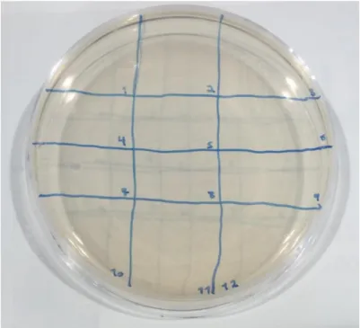
At the beginning of the experiment all 12 strains were streaked on agar plates, which were left to grown at 32ºC for 48 hours. After this time, 12 isolated colonies from each strain were picked to undergo Mutation Accumulation (MA). These were again streaked on new agar plates in order to pick isolated colonies once more, in a process of bottlenecking. (Trindade, Perfeito, & Gordo, 2010) An example of these agar plates can be seen in Figure 2.1. All 12 lines for each strain underwent this bottlenecking every 48 hours and were frozen every 12 bottlenecks.

Figure 2.1 Example of YES agar plate used to streak each strain’s 12 cell lines. The grid pattern allows us to streak all 12 on the same plate, one per area.

The number of generations that occur per bottleneck were estimated during previous experiments at the lab by counting the number of Colony Forming Units present in a colony after the usual 48 hours of growth (Nf). Assuming each colony originates from a single cell, the number of generations elapsed will

equal log2(Nf). These calculations estimate each bottleneck corresponds to 16 generations, which means

after 48 bottlenecks 768 generations have elapsed and 144 bottlenecks equal 2304 generations (A. P. Marques, personal communication).

C2, along with C8, are the only strains not to have 12 lines past bottleneck 48 (B48). Whenever a streaked colony fails to produce growth during a bottleneck, we go back to the previous bottleneck’s plate and collect a new isolated colony, in order to recover the line and keep all 12 lines for each strain accumulating mutations throughout all bottlenecks. If the new colony is also unable to grow during the

(24)

10 next 48 hours, we once again go back to pick up yet a third isolated colony. However, if this happens a third time, we consider that line to have gone extinct, i.e., that the deleterious mutations it has accumulated have reached the threshold of lethality and will not allow viable daughter cells to replicate. We perform this recovery three times to ensure that the line is really lost due to deleterious mutations and not to a technical problem. We take note of which line went extinct and proceed with the experiment for the remaining ones. In this case, line C2.12 went extinct at bottleneck 132, so it is not represented in the data for bottleneck 144 (B144) competitions.

The MA propagation was carried out by myself and two other members of the lab: Simone Delgado and Paula Marques.

2.3 Assessment of the number of cells picked during MA

An MA experiment is aimed at reducing selection as much as possible in order for mutations to accumulate close to the rate at which they appear. In microorganisms, this involves isolating single colonies and re-streaking them. Ideally each colony is the result of the growth of a single cell. To test whether this was the case in our experiment, we devised a protocol to assess the probability of carrying, and streaking, colonies which had grown from one single cell.

Three different S. pombe strains were grown from -80ºC stocks, all variants of C4 of the same mating type and with different fluorescence markings: one marked with mCherry (the same used as the reference for competitions), one with GFP and the last unmarked (the same used in the MA experiment). These were grown on YES agar for 48 hours at 32ºC, after which a piece of growth from each was placed in 5mL liquid YES and grown in a shaker at 32ºC for 48 hours once more. From those cultures, which were presumably at similar concentration levels, 100µL of each were pipetted into an Eppendorf tube and mixed through up-and-down. Then, 5µL pipette tips were dipped in this solution and then simply touched upon a plate of YES agar. This size was chosen to produce a small droplet that gave rise to colonies close in size to the ones obtained during Mutation Accumulation experiment. The MA experiment was carried out by three different people in the lab and so we tested the streaking technique for every user. 96 such colonies were made for each one, to test all three individual techniques. We replicated the movements we used for each bottleneck: divided a YES agar plate into 12 sections and picked material from one mixed colony, streaking it inside one section.

Although they had come from mixed cultures, by streaking each colony we expected to isolate single cells. After another cycle of growth at 32ºC for 48 hours we picked one colony from each section and streaked it once more onto new YES agar plates. If the streaking isolated single cells, then the resulting growth would present only one fluorescent marking per section; if not, then we would distinguish two

(25)

11 or three different colors in each. One final cycle of growth later, the plates were observed under the UV light of a Zeiss Stereo Lumar microscope. We then counted how many sections had only red growth, only green, only grey (not marked) growth, a mix of two colors or a mix of all three.

While calculating the odds of carrying a certain number of cells, we also had to take into account the possibility of carrying two or more cells with the same fluorescence. For example, a completely red colony might have grown from only one mCherry-marked cell, or it might also have grown from two or more mCherry-marked cells. A green and red colony must have been originated by at least one mCherry and one GFP-marked cells, or it could also have been formed from two or more mCherry-marked and one GFP-marked cells, two or more GFP-marked and one mCherry-marked cells or even multiple cells from each fluorescence type.

Due to the complexity of this estimation, we decided to use a Markov Chain Monte-Carlo (MCMC) algorithm to calculate the most likely probabilities for carrying any number of cells. This algorithm allows us to approximate an unknown probability distribution of our system at steady-state. By chaining together known probabilities starting from a known initial state, a trajectory to a final state can be simulated. Simulating many trajectories and many final states, and averaging the results, allows us to estimate the unknown probability distribution for the steady-state of our system (Fonnesbeck, 2014). This analysis was performed with the help of PhD student Diogo Santos.

As we perform MA on round plates, the grids we streak colonies in have rounded corners (Figure 2.1). We wanted to test whether the smaller streaking area would lead to a higher number of mixed colonies. We performed a χ2_{test to verify whether the number of mixed colonies in these corners was significantly}

higher than that of the other area of the grid.

2.4 Freezing and unfreezing samples

We froze a sampleof each cell line every 12 bottlenecks, to have material for competition assays and to serve as backup, or “fossil record”.

In order to freeze the samples, the first pipette tip used to make the first streak in the agar during MA was dipped into 500µL of liquid YES in a 96 Deep Well plate. These plates were then grown in a shaker at 32ºC for 48 hours. Afterwards, the plates were centrifuged at 3500 RPM for 5 minutes, so as to conserve the maximum amount of cells when freezing. The supernatant was removed and the pellets resuspended in 150 µL Freezing Medium (FM), a 1:1 mix of liquid YES with a 50% glycerol solution. The resulting suspension was pipetted into a 96 well plate, precooled on dry ice, and then stored at -80ºC.

(26)

12 When samples were needed, the 96 small well plates holding frozen samples were carried outside of the -80ºC freezer while being kept on dry ice, so as to have the cells at room temperature for as little time as possible, as glycerol is toxic above freezing temperatures. Samples were taken from 48 wells at a time with the help of a replicator, whose tips had previously been sterilized by being dipped in pure alcohol, brought to a flame, and allowed to cool down before being inserted into the wells and then, carrying a droplet of the frozen samples of each tip, touched upon the surface of a YES agar plate. After that, the 96 small well plate was returned to its place in the -80ºC freezer as quickly as possible and the agar plates were placed at 32ºC for 48 hours.

2.5 Fitness Assay

All fitness measurements were performed by competing test strains against a reference. All competitions assays were started from frozen samples, so as to keep consistency across all experiments. We measured competitive fitness for the ancestral strains (pre-MA), as well as all lines from bottlenecks 48 and 144 (B0, B48 and B144, respectively).

Every sample was competed against a reference strain marked with mCherry fluorescent marker. Both the competing cell lines and the reference strain were grown on YES agar plates at 32ºC for 48 hours. Then a bit of growth was placed in a well in a 96 Depp Well plate containing 500µL liquid YES, whereupon they were placed once more at 32ºC in a shaker for 24 hours. These wells were well mixed by pipetting before having their contents mixed in a well containing 180µL PMG in a 96 small well plate. Each well received 10µL of the reference strain and 10µL of the competing line. Though this 50/50 mix was the general case, some lines demanded different mix ratios, as explain in the next page. From this mixture, 20µL were placed in 500µL liquid YES in the corresponding well of a new 96 Deep Well plate, which went on to grow in a shaker at 32ºC for 24 hours. The remaining 180µL were used to estimate cell numbers by FACS, following incubation for at least 2 hours in PMG This measurement was the first timepoint of the competition. Every day, during 7 days the cells were diluted in PMG and transferred to a new deep-well plate and placed at 32C. Hence, for each competition, we have 8 different time points.

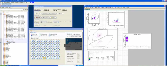
The measurements were performed through Fluorescence Activated Cell Sorting (FACS) with LSR Fortessa equipment. This device is customizable with up to four lasers with modulable wavelengths and offers excellent sensibility and resolution (Becton et al., 2011), making it ideal to measure small particles such as yeast cells. The software is easy to use and calibrate, and the machine itself quickens our research, as it can automatically reads complete 96 small well plates. Moreover, this method allows us to analyze 10 000 cells in less than 1 minute, giving us a strong statistical confidence.

(27)

13 We used two different lasers and wave-length receptors: one optimized for GFP and the other for mCherry. GFP was detected with a 488nm laser using a 530/30 nm bandpass filter, while mCherry was detected with a 561 nm laser using a 630/30 nm bandpass filter. The equipment was calibrated, with bi-weekly adjustments performed during maintenance, by the IGC Flow Cytometry Unit.

On the software’s interface we define three windows (Figure 2.2), each with a gate to select cells of interest: the first to separate viable yeast cells from contaminations and cell debris; a second to separate singlets from cell aggregates; and a third to separate mCherry-marked cells from unmarked ones. This gave us a ratio, and a percentage, of how many unmarked cells there are, comparatively to the number of mCherry cells, there are in the mixture at each timepoint. If this number steadily increases across timepoints, it means the line’s fitness is superior to the reference’s; if it decreases, it means it’s inferior.

Figure 2.2 LSR Fortessa interface, showing an example of a well’s cells being separated through the three windows and between the mCherry-marked reference competitor and the interest sample strain.

Mixtures that reached mcherry frequencies higher than 99% or lower than 1% within few timepoints were not used in the experiment. This threshold was chosen because pure cultures of either mCherry or unmarked cells had around 1% of cells in the other gate. We used only those competitions that went through at least 3 timepoints before reaching those frequencies. For that effect, the replicate was repeated with different initial ratios of cells, adding less of the fittest competitor and more of the least fit (always in a total of 20µL) so as to delay one strain’s dominance over the other.

The change in ratio of unmarked/mCherry cells across timepoints was then used to estimate fitness levels. If we assume exponential growth, then:

(28)

14 where N(t) is the number of cells at time t and W is the fitness of those cells. This equation can also be written as

Equation 2 𝑾𝒕 =_𝑵(𝟎)𝑵(𝒕)

We define relative fitness as

Equation 3 𝑾𝑹= _𝑾𝑾𝒎

𝑾𝑻

where WR is the relative fitness of the unmarked (m) strain when compared to the reference strain (WT),

then by combining equations 1 and 2 we have

Equation 4

𝑾

_𝑹𝒕

=

𝑵𝒎(𝒕) 𝑵𝒎(𝟎) 𝑵𝑾𝑻(𝒕) 𝑵𝑾𝑻(𝟎) or, simplifying Equation 5 𝑾_𝑹𝒕 = 𝑵𝒎(𝒕)∗𝑵𝑾𝑻(𝟎) 𝑵𝒎(𝟎)∗𝑵𝑾𝑻(𝒕)

We can take into account that the proportion of one type of cell is inversely proportional to the amount of its competitor present in the environment, and that the sum of both strains will equal 100% of the cells present in the environment. Ergo, if we define p(t) as the frequency of unmarked cells at time t and

1-p(t) as the frequency of reference mCherry cells, we have

Equation 3 𝑾_𝑹𝒕 = 𝒑(𝒕)[𝟏−𝒑(𝟎)]_{𝒑(𝟎)[𝟏−𝒑(𝒕)]}

These calculations revolve around the curve measuring the percentage of each type of cells, marked and unmarked, in the medium. If we linearize this curve, we can directly correlate its slope with the relative fitness of the strains.

Equation 4 𝒍𝒏(𝑾_𝑹𝒕) = 𝒍𝒏( 𝒑(𝒕)[𝟏−𝒑(𝟎)]_{𝒑(𝟎)[𝟏−𝒑(𝒕)]} )

Defining the selection coefficient, s, as

Equation 5 𝒔 = 𝐥𝐧 𝑾𝑹

𝒕 𝒕 from equation 4 we get

(29)

15 Equation 5 defines a linear relationship between the natural logarithm of the ratio of frequencies and time (measured as number of generations for the reference, 8 per timepoint). By performing least squares linear regression we can estimate the slope of this line which gives us s. We can then estimate fitness using equation 4.

The mCherry reference strain has a fitness of 1 by definition, and the fitness values of all lines can be read as a comparison of that line’s ability to survive and thrive in liquid YES when compared with the reference’s own. For example, C4B0 possesses the fitness level closest to one, at 0.992±0.003, apropos of being the most similar to the competing reference strain, which is a variation of C4 with the added mCherry fluorescent marker.

It should be noted that SPP20B0 fitness values had been measured during previous experiments at the laboratory, before the beginning of this Thesis’ work, using the same methods used for all other strains.

2.6 Statistical analysis and parameter estimation

Between those bottlenecks whose lines’ distribution of fitness values followed a Normal distribution, the data could be analyzed with Welch’s T-test. To compare non-Normal datasets, or Normal datasets with not-Normal ones, we used the Kolmogorov-Smirnov’s (KS) test. However, considering all bottleneck levels, including the ancestrals, had at least one not-Normal distribution, KS test was used to compare the distributions of all data pairs, to keep consistency across all analyses. KS test, as a non-parametric test, is also more conservative than T-test, giving us a greater certainty that the differences we find are actually significant.

Due to the fact that the median of each strain’s fitness distribution changes throughout the experiment, and not just the distribution’s shape and spread, we decided to also perform a test more sensitive to this last parameter. The significance of this value was calculated through the Mann-Whitney-Wilcoxon (Wilcox) Test. This way, we are sure the change is one of variance and of the average of all 12 lines’ fitnesses.

Bonferroni corrections were applied by multiplying the p-value by the number of tests performed. Using fitness data, we estimated the mutation parameters for each strain: the average fitness decline caused by each deleterious mutation (sd), the mean number of arising deleterious mutations per

generation (Ud) and the mean number of mutations ((G)) present at each generation (G). This was

accomplished using the same methods as in Trindade et al. to estimate mutation parameters in Escherichia coli (Trindade et al., 2010; Gordo & Dionisio, 2005; Colato & Fontanari, 2001):

(𝐆) = 𝑼𝒅

𝒔𝒅(𝟏 − (𝟏 − 𝒔𝒅) 𝑮

(30)

16 And sd and Ud can be calculated through 𝒔𝒅=

𝒎𝟐

𝒎𝟏 and 𝑼𝒅= 𝒎𝟏 (𝟏−(𝟏−𝒔𝒅)𝑮

where m1 is the slope of the natural logarithm of the mean fitness of all lines with bottleneck number and m2 is is the slope of the natural logarithm of Fi with bottleneck number i. Fi can be calculated with the formula

𝑭𝒊 =𝑾𝒊̅̅̅̅̅̅𝟐 𝑾𝒊 ̅̅̅̅𝟐

W corresponding to the mean fitness of each individual line at bottleneck i.

This model assumes no beneficial or compensatory mutations arise, only deleterious mutations, each with a selection coefficient sd. Knowing the slopes m1 and m2 and their respective standard error (δ),

one can estimate associated errors for Ud and sd, calculated through error propagation as

In order to test which backgrounds behave differently from each other, we fitted an Analysis of Variance Model (ANOVA) to check how the change in fitness (fitness at B0 subtracted from fitness at B144) correlated with each individual background.

All analysis were performed in Microsoft Excel or R Studio.

Mutation parameters could not be estimated for strain SPP20, for which only two of its bottlenecks’ fitness levels were measured; to perform adequate calculations, at least three data points are necessary. The formulas used were also not applicable to strains C2 and T4 because these strains show strong signs of accumulation of beneficial mutations.

2.7 Tetrad Dissection

In order to test whether the mutations accumulated during the experiment were epistatic, i.e., whether they interacted, we crossed two evolved lines with an ancestral. This allowed us to separate the

(31)

17 accumulated mutations and directly test whether their effects were epistatic or additive. For that effect, we chose mutated lines from strains T4 (namely, T4.11) and C4 (namely, C4.3) from bottleneck 48. T4.11 was chosen due to its apparent beneficial mutations, and C4.3 was the most divergent C4 line at bottleneck 48 and hence the most likely to have accumulated mutations. These had to be crossed with an unmutated background, i.e. one at bottleneck 0, and the only strain used in this experiment of the opposite mating type was C5. We will call these two crosses C5/C4.3 hybrids and C5/T4.11 hybrids. However, we needed to control for possible epistatic effects in the ancestral backgrounds. As such, we repeated the experiment with just unmutated strains. We crossed the same ancestral C5B0 with ancestral C4B0 and separately with T4B0. These crosses will be referred to as C5a/C4a hybrids and C5a/T4a hybrids, respectively.

As for the mating process itself, in order to mate, S. pombe haploids must be starved of nutrients(Nurse, 2000) specifically nitrogen (Forsburg & Rhind, 2006), or they will opt for asexual reproduction. For that effect, we unfreeze and take a bit of cellular growth of the strains we want to cross, grown in YES agar, and place it in 100µL PMG. We do a short centrifugation (1 minute at 3000 RPM) to form a pellet and take pipette the supernatant out. This process will clean the cells of nutrients they’d carry from the YES agar and is necessary for mating to occur. However, our strains tend to produce few spores, so we needed to increase the efficiency of the process. In order to do so, we starved our cells further. We did so by resuspending the pellet in a fresh 100µL PMG and letting it settle for half-an-hour/one hour,

This process leads the cells to consume their internal supplies of nutrients and to excrete their waste into the medium, which we remove. As such, they will go onward to be deposited onto the mating medium with no resources that would stimulate them to replicate instead of mate.

Once all cell samples were properly starved we mix resuspend them by up-and-down before pipetting 10µL of each into a new Eppendorf tube, where we mix the two we want to cross before pipetting 10µL of this mix onto mating medium. The droplets are allowed to dry by the flame before the plate is closed and sealed with parafilm and placed at 25ºC for 48 hours. After these have passed, we take the plate out and take a bit of the colonies formed, one per mixture, to check under the microscope whether they’ve formed tetrads.

If successful, we suspend a portion of the growth on ≈30µL PMG and pipette it onto a YES agar plate, which we tilt to form a line dividing the plate in two. It is on this plate that we dissect the tetrads, using Singer’s MSM 400 Manual Dissection Microscope and following Paul Nurse’s Fission Yeast Handbook’s instructions (Nurse, 2000). Once the tetrads are dissected, we leave the plate growing at 32ºC for 48 hours, upon which we’ll have isolated colonies, each descended from a single spore.

(32)

18 These colonies were frozen using the same methods as those derived from MA, with the only difference being that the whole colony was put into liquid YES to grow. These frozen samples were also competed according to the methods described previously for MA samples.

2.8 Comparisons between fitness and genotype

Just as two parental genomes are combining and interacting to form new distributions of fitness effects, this recombination can be seen in certain phenotypic characteristics associated with known genetic markers. As our strains have auxotrophic markers that allow us to distinguish different backgrounds, testing which phenotype they express and, from that, know whether the recombinant spores inherited their genotypes from one of the parental strains or whether they possess a mix of both. Namely, our strains are characterized by their ability, or inability, to grow on media lacking arginine, lysine and/or histidine. We can produce selective media by not adding one of these aminoacids to PMG plates and by verifying which of these media the samples derived from tetrad dissection can grow on, find out whether their phenotype is similar to that of one of the parental strains or a mix of both.

From this data we were able to calculate each cross’ recombination rate by dividing the number of spores with a mixed genotype by the total number of spores.

Using an Analysis of Variance Model (3-Way ANOVA), we also estimated the impact each marker has on the recombinant spore’s fitness, for all 4 crosses.

(33)

19

3. Results

3.1 Assessment of the number of cells picked during mutation accumulation

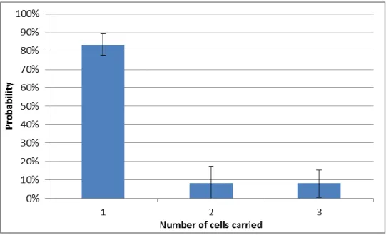
In order to investigate whether the genotype and karyotype affect the spontaneous mutation rate in fission yeast, we performed a mutation accumulation experiment (MA). In an MA, natural selection is reduced to a minimum, such that mutations accumulate close to the rate at which they are generated. To do so in microorganisms, this typically involves picking up one colony, re-streaking it in such a way that a new colony can be isolated after growth (Kibota and Lynch, 1996). This is called a bottleneck, whereby the population is reduced from several billion to a few cells, ideally only one. To make sure no more than one clone was being streaked, we estimated the number of cells carried over in each bottleneck. To do so, we mixed cells carrying three different fluorescent proteins, performed a bottleneck in the same manner as in the MA and checked how many colonies had mixed fluorescence (see Material and Methods, section 2.3).

Figure 3.1: Probability of isolating one, two or three cells per bottleneck. The error bars represent standard deviation from the mean. The data represents the pooled results of three

experiments, each analyzing 96 streaks

From the frequency of colonies with 1, 2 and 3 fluorescent proteins, we estimated the probability of isolating 1, 2 or 3 cells. On average, at each bottleneck we isolate a single cell 83% of the time (±5%). This means 17% of the colonies originate from two or more cells. While this suggests that there can be some level of natural selection during the MA, that selection is still small, as the effective population

(34)

20 size is still close to unity. Even if two cells are dragged together during the streaking, it is very possible they were sister-cells, carrying similar, if not identical, genotypes. Furthermore, the chance of carrying more than one cell twice in a row for any given line is of less than 3%; the chance of doing so thrice in a row is about 0.5%.It is unlikely that a cell line will be subjected to multiple passages with this increase in selective pressure without complete isolation occurring in-between them.

We also tested whether the position of the colony in the petri dish affected the number of cells per bottleneck. We streak 12 lines on each YES agar plate, along a grid. The grid squares near the edge are smaller in size relative to the remaining areas. This smaller space could potentially lead to smaller streaks and, consequently, worse cell separation and fewer chances of obtaining colonies grown from isolated cells. Although the number of mixed colonies was indeed slightly higher in the corners than other regions (12 mixed colonies in corners, compared to 9 in all other fields), a χ2_{test indicated that the}

difference is non-significant (p-value > 0.1 ).

3.2 Mutation accumulation and competitions

We performed the MA experiment for 12 different strains, each in 12 different replicate lines (144 evolution lines total). Of these 12 strains, 2 of them are direct descendants of the fission yeast type strain L972 where the only genetic engineering done to them was the introduction of a clonat resistance in the mating type locus (Avelar et al., 2013). One of them (SPP27) was a gift from the I. Tolic in Gottingen, Germany, while SPP26 was kept in the Portuguese Yeast Culture Collection under the number PYCC4197. These 2 strains have the same karyotype (A. T. Avelar, personal communication). However, whole genome sequencing done in our lab showed 16 genomic differences (not shown). From here on, these will be called the “Wild Type-like strains”. The other 10 strains represent pairs of strains where one of them has a chromosome rearrangement (1 inversion and 4 translocations) and the other is its wild type control. The controls have the same karyotype as the wild type and contain the loxP cassettes in the same locations as the rearranged strains. The construction of these strains and their karyotypes are described in Avelar 2013 and the materials and methods section. We use the same nomenclature for the rearrangements as in Avelar 2013.

We measured competitive fitness (see Materials and Methods, section 2.5) for all 12 strains at time 0 and for all 156 lines after 48 and after 144 bottlenecks (approximately 768 and 2304 generations respectively). The fitness values for all replicates of each strain and every line can be seen in Tables 6.2 through 6.14 in the Supplementary Material.

Figure 3.2 shows the fitness trajectory for the wild type strains SPP26 and SPP27. At time 0 they differ slightly in fitness with SPP27 being significantly less fit.

(35)

21

Figure 3.2 Average fitness trajectories for strains SPP26 (in light blue) and SPP27 (in dark blue) across three different bottleneck numbers: B0, B48 and B144. For B0 the error bars represent experimental error from several measurements of the ancestral strain, while for B48 and B144 they represent the variance between all 12 cell lines per strain. * shows a significant change in fitness distributions between both bottleneck numbers, while Δ does the same for fitness average. */Δ p-value < 0.05; **/Δ Δ p-value < 0.01; ***/Δ Δ Δ p-value < 0.001. Bonferroni corrections were applied to all p-values.

Strain SPP26’s fitness decreased from 1.067 ± 0.006 (average ± standard deviation) (normally distributed) at B0 to 1.06 ± 0.02 (not normally distributed) at B48 and to 1.04 ± 0.04 (not normally distributed) at B144. Strain SPP27’s fitness decreased from 1.046 ± 0.004 (normally distributed) at B0 to 1.040 ± 0.006 (normally distributed) at B48 and to 0.80 ± 0.05 (not normally distributed) at B144. On average, SPP26 did not decrease in fitness, while SPP27 did, especially between bottlenecks 48 and 144.

Figure 3.3 shows the fitness trajectory for strains I2 and C2. At time 0 they differ slightly in fitness with C2 being significantly less fit.

(36)

22

Figure 3.3 Average fitness trajectories for strains C2 (blue) and I2 (red) across three different bottleneck numbers: B0, B48 and B144. For B0 the error bars represent experimental error from several measurements of the ancestral strain, while for B48 and B144 they represent the variance between all 12 cell lines per strain. * shows a significant change in fitness distributions between both bottleneck numbers, while Δ does the same for fitness average. */Δ value < 0.05; **/Δ Δ p-value < 0.01; ***/Δ Δ Δ p-p-value < 0.001. Bonferroni corrections were applied to all p-p-values.

Next, we compared the fitness trajectories for Inversion 2 (I2 – see Introduction, section 1.3) and its control, C2. Strain I2’s fitness decreased from 1.06 ± 0.01 (normally distributed) at B0 to 1.040 ± 0.007 (normally distributed) at B48 and to 1.00 ± 0.05 (not normally distributed) at B144.

Strain C2’s fitness increased from 1.026 ± 0.010 (normally distributed) at B0 to 1.05 ± 0.02 (not normally distributed) at B48 and decreased to 1.02 ± 0.06 (not normally distributed) at B144.

I2B48 and C2B48 do not have significantly different averages nor distributions, and the same happens between I2B144 and C2B144. This indicates the two strains are converging.

We should note than C2 only has 11 lines past bottleneck 132. One of the lines went extinct (see Materials and Methods, section 2.2).

Figure 3.4 shows the fitness trajectory for strains T4 and C4. At time 0 they are significantly different in fitness, with T4 being less fit.

(37)

23

Figure 3.4 Average fitness trajectories for strains C4 (blue) and T4 (red) across three different bottleneck numbers: B0, B48 and B144. For B0 the error bars represent experimental error from several measurements of the ancestral strain, while for B48 and B144 they represent the variance between all 12 cell lines per strain. * shows a significant change in fitness distributions between both bottleneck numbers, while Δ does the same for fitness average. */Δ p-value < 0.05; **/Δ Δ value < 0.01; ***/Δ Δ Δ value < 0.001. Bonferroni corrections were applied to all

p-values.

Strain T4’s fitness increased from 0.88 ± 0.02 (normally distributed) at B0 to 0.913 ± 0.007 (normally distributed) at B48 and to 1.02 ± 0.02 (normally distributed) at B144. This result is unexpected and very surprising. Due to the absence of natural selection and the fact that most mutations are deleterious, we do not expect fitness to increase consistently in MA experiments.

Strain C4’s fitness decreased from 0.992 ± 0.003 (normally distributed) at B0 to 0.98 ± 0.01 (not normally distributed) at B48 and to 0.97 ± 0.01 (normally distributed) at B144.

Figure 3.5 shows the fitness trajectory for strains T5, SPP20 and C5. At time 0 they are significantly different in fitness, with SPP20 being less fit than C5 and T5 being less fit than both.