On cluster analysis of complex and heterogeneous data

On Cluster Analysis of Complex

and Heterogeneous Data

Helena Bacelar-Nicolau1, Fernando C. Nicolau2, Áurea Sousa3 and Leonor Bacelar-Nicolau4

1

University of Lisbon, Faculty of Psychology, LEAD; ISAMB; Lisbon, Portugal Email: hbacelar@psicologia.ulisboa.pt

2

University of Lisbon, FCT, Department of Mathematics, Caparica, Portugal Email: fernandonicolau@netcabo.pt

3

University of Azores, Dep. of Math., CEEAplA, Ponta Delgada, Azores, Portugal Email: aurea@uac.pt

4_{University of Lisbon, Faculty of Medicine, Institute of Preventive Medicine, ISAMB,}

Lisbon, Portugal Email: lnicolau@fm.ul.pt

Abstract: Cluster analysis or “unsupervised” classification (from “unsupervised learning”,

in pattern recognition literature) usually concerns a set of exploratory multivariate data analysis methods and techniques for grouping either statistical data units or variables into groups of similar elements, that is finding a clustering structure in the data. Classical clustering methods usually work with a set of objects as statistical data units described by a set of homogeneous (that is, of the same type) variables in a two-way framework. This paradigm can be extended in such way that data units may be either simple / first-order elements (e.g., objects, subjects, cases) or groups of / second-order or more elements from a population (e.g., subsets, samples, classes of a partition) and/or descriptive variables may simultaneously be of different (e.g., binary, multi-valued, histogram or interval) types. Therefore, one has a complex and/or heterogeneous data set under analysis. In that case classification will often be carried out by using a three-way or a symbolic/complex approach. The present work synthesizes previous methodological results and shows several developments mostly regarding hierarchical cluster analysis of complex data, where statistical data units are described by either a homogeneous or a heterogeneous set of variables. We will illustrate that approach on a case study issued from the statistical literature. The methodology has been applied with success in a data mining context, concerning multivariate analysis of real-life data bases from economy, management, medicine, education and social sciences.

Keywords: Three-way data, Symbolic data, Interval data, Cluster analysis, Similarity

1 Introduction

In complex and large data bases, we are very often concerned with matrices where data units are described by some heterogeneous set of variables. Therefore, the question arises of how we should measure the similarity between statistical data units in a coherent way, if different types of variables are involved. Traditionally, partial similarity coefficients for each type of variables are computed, and then a convex linear combination of those similarities gives a global similarity between data units. Such procedures should be performed in a consistent way, combining comparable similarity coefficients in a valid / robust global similarity. Clustering data sets where mixed variables types are involved has interested many

researchers. In two-way data matrices a well known coefficient for comparing

subjects described by different types of variables was already proposed in 1971 by Gower. Cluster analysis of symbolic data described by mixed variables types may be found, for instance, in Bacelar-Nicolau et al. (2009, 2010) and in De Carvalho and Souza (2010), while Chavent et al. (2003) concerns clustering of interval data, which plays a special role in this paper. A number of dissimilarity coefficients, like adaptive squared Euclidean, city-block, Hausdorff distances or generalized Minkowski metrics, among others, may be found in those papers, either in a hierarchical or in a non hierarchical clustering context. In this paper, we deal with a consistent global affinity coefficient as the basis of hierarchical clustering methods (Bacelar-Nicolau, 2002; Bacelar-Nicolau et al., 2009, 2010). The next section gives a brief description of our approach to three different types of variables commonly found out in real databases, the third section illustrates a case study that partially applies the methodology and the last section concerns conclusions and some developments.

2 Complex and Heterogeneous Data

Let D = {1,…,n} be a set of n statistical data units which are described by a set of p

variables, Y = {Y1, ...,Yp}. Cluster analysis usually aims to obtain a classification of

one of the two data sets, either D or Y, given the other one. Here we will be concerned with clustering models on the set of data units D. The data units can be either simple elements (e.g., subjects, individuals, cases) or subsets of objects in some population (e.g., subsamples of a sample, classes of a partition, subgroups of the population). Such kind of data might be represented in a generalized three-way data matrix where the k-th row, (k=1,… ,n), gives the description of the k-th data unit by the p variables, and the (k,j)-th entry, (k=1,… ,n ; j=1,…,p), may contain for instance a finite number of real values, a frequency distribution, a probability distribution or an interval of the real data set R, instead of one single value. In most mixed or heterogeneous data sets we have been studying, those values concern discrete, binary or interval types of variables, either conjointly or in two

by two type combinations. Hence in the set Y = Y1,...,Yj,..., Yj’,..., Yj’’,...,Yp of p

variables, we will assume that Yj represents a discrete or a categorical (modal)

mj’ –dimensional binary vector and Yj’’ is an interval variable, where j, j’ and j’’ belong to {1,…,p} (e.g., Bacelar-Nicolau, 2000; Bacelar-Nicolau et al., 2009, 2010). Thus the corresponding generalized columns have n rows, and the k-th row

(k=1,… ,n) contains: for Yj , a frequency distribution





j

kjm kj n

n ₁,..., , where

n

kj is

the number of subjects in the k-th data unit who share the



-th category ofthe j-th

variable; for Yj’ , an element

 

'

1 , 0 mj

k of the power set

 

' 1 ,

0 mj , the whole binary

sub-table being an element of

 

_0,1nmj'; for Y_j’’ , an interval I_kj’’ of the real axis.

Thus the data set may be represented by the following generalized table:

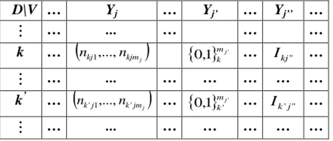
Table 1. Generalized three-way data matrix with heterogeneous variables

D\V … Yj … Yj’ … Yj’’ …  … ... … … … k …



nkj1,...,nkjmj



 

' 1 , 0 mj k … Ikj'' …  … ... … … … … … k’ …



nk'j1,...,nk'jmj



…

 

' ' 1 , 0 mj k … Ik' j'' …  … ... … … … … …

Therefore, a consistent global similarity (or dissimilarity) coefficient should be used for such mixed types of data.

2.1. Discrete and categorical variable

Let Yj be a discrete or a categorical (modal) variable with mj (



=1,...,mj)

modalities. Then, its general k-term (k=1,…,n) may be obtained by simply

replacing

x

_kjby the frequency

n

_kj of the



-th category or modality (



=1,...,mj).

The relative frequencies

p

kj



n

kj

n

kj,



=1,...,mj, generate a discrete probability

distribution, that is a profile, or else a histogram, ((m1,pkj1

), …,

(mj, pkjm_j

))

.

Therefore, in order to measure partial/local similarity between each pair (k, k’) of data units, over a modal variable, one may choose a similarity (or a dissimilarity) coefficient for probability distributions (e.g., Bock and Diday, 2000; Bacelar-Nicolau, 2000).

2.2. Binary vector

Let us now take variable Yj’, a mj’ – dimensional binary vector (see Table 1). Given

the data units k and k’, let us represent by sj’ the cardinal of positive agreements

and vj’ the cardinals of disagreements (respectively,

x

kj'_=1,

x

k' j'=0 and

x

kj'=0, 

' ' j k

x

=1). Then, we also have: _'

1 ' '' ' j m j k kj j x x s   , '1' (1 ')(1 '') j m j k kj j x x t    ,    ' 1 ' ' ' ' j (1 ) m j k kj j x x u    and    ' 1 ' ' ' ' (1 ) j m j k kj j x x v   .

One can find quite a large list of coefficients for binary data in the statistical literature, computed from those cardinals. Thus, a local similarity coefficient for a pair of rows (k, k’), k, k’=1,…,n, over a binary vector, may be computed from the

22 contingency table associated with the pair (k, k’) in the j’-th binary sub-table,

as follows:

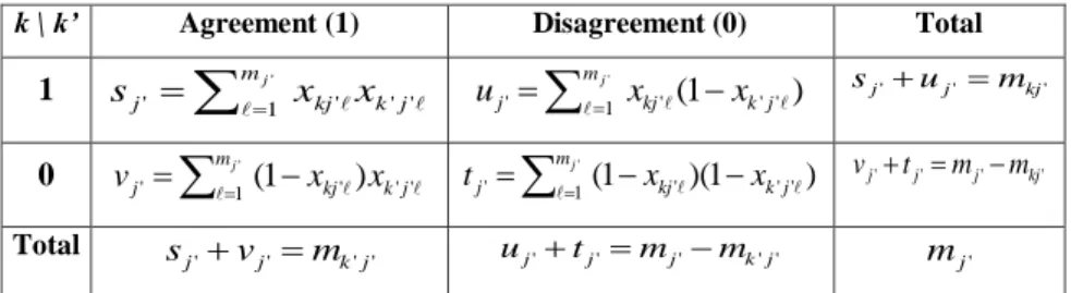
Table 2. Table of agreements and disagreements for a binary vector k \ k’ Agreement (1) Disagreement (0) Total

1 



_' 1 ' ' ' ' j m j k kj j x x s _{  } 



_'  1 ' ' ' ' (1 ) j m j k kj j x x u _   sj'uj' mkj' 0 



_'  1 ' '' ' (1 ) j m j k kj j x x v _   



_   ' 1 ' '' ' (1 )(1 ) j m j k kj j x x t _   vj'tj'mj'mkj' Total ' ' ' ' j kj j v m s   uj'tj'mj'mk'j' mj'

where

m

_kj' (

m

_{k' j'}) denotes the cardinal of presences in the data unit k

(respectively, k’) for the binary vector Yj’.

2.3. Interval-type variable

A variable Yj’’ defined on the set D of statistical data units is an interval variable if

for all kD the subset Yj’’ (k) is an interval of the real data set R. Let Yj’’ be an

interval variable associated with a generalized column j’’ (see Table 1), where

each cell (k, j’’) contains an interval

I

_kj''(k =1,…,n).

Let

I

j'' be the union of the intervals

I

kj''

:

I

j''





I

kj'' (k =1,…,n). Thus,

I

j'' is

the domain of Yj’’. Let



I_j'': 1,...,m_j''



be a set of mj’’ elementary intervals,

such that the following properties hold, for



,



'



1

,....,

m

_j''

,







'

;

k



1

,...,

n

:

i)I_j''I_j''; ii) I_j''I_j'''



; iii) I_kj''I_j'' I_j'', if I_kj''I_j'' 



, and



  ''_ '' j kj I I , otherwise.

Let

x

_kj'' be x_kj''  I_kj''I_j'' , where   represents the interval range. Then,

    '' '' '' '' '' j if Ikj j j kj I I I x    , andx_kj'' 0, otherwise.

Therefore, one has for each pair (

I

_kj'',

I

_{k' j''}) of intervals: x_kj''  I_kj'' , '' ' j k ' j' k' I x  and



j1'' '' ' ''



''



' '' m j k kj j k kj

x

I

I

x

   . Consequently, the (k,k’)-th

pair of intervals in the j’’-th generalized column of Table 1, can be associated to a

generalized 22 contingency table as follows:

Table 3. Table of agreements and disagreements for interval variables k \ k’ Agreement Disagreement Total Agreement

s

_j''



I

_kj''



I

_k'j''

u

j''



I

kj''



I

kc'j''

s

j''



u

j''



I

kj'' Disagreement

v

_j''



I

_kjc_''



I

_k'j'' kcj c kj j

I

I

t

''



''



' '' c kj j j

t

I

v

''



''



'' Total

s

_j''



v

_j''



I

_k'j''

u

_j''



t

_j''



I

_kc_'j''

I

_j''

Into the cells of Table 3, agreements or disagreements are measured by the respective interval ranges, instead of the cardinals computed for a binary vector.

Note that

I

kjc'' represents the complementary interval of

I

kj'' in the domain

I

j''.

2.4. Global affinity coefficient

The three approaches above for representing binary, modal and interval valued variables lead to a comprehensive approach for measuring global proximity between complex data units (k, k’) described by those heterogeneous kinds of variables. A special interesting case arises when only binary and interval valued variables are present in a database, since then all (the large list of) association

coefficients for binary data defined from the 22 related contingency table can also

be used in exactly the same way for interval data, from the corresponding

generalized 22 contingency table. If modal variables are also present in the

database, a global proximity coefficient between (k, k’) has to consistently take in account proximity between histograms as well. The affinity coefficient responds to those requirements.

The affinity coefficient was formerly introduced by the pioneer work of K. Matusita, started with Matusita (1951) for measuring proximity between two probability distribution functions. It is related to a special case of the Hellinger (or Bhattacharyya) distance. We have extensively studied the affinity coefficient and its properties, several affinity generalizations and some particular cases in cluster analysis context (e.g., Bacelar-Nicolau, 2000, 2002; Bacelar-Nicolau et al., 2009,

2010). The weighted generalized affinity coefficient a(k,k'), between a pair of

statistical data units k, k’  D (k, k’=1,…,n), may be defined in a three-way

context, as the weighted mean of local / partial affinities between k and k’ over the











          mj j k j k kj kj p j j p j x x x x j k k aff k k a ₁ ' ' 1 1 j , '; ) ' , (   _   (1)

where the sum named aff (k,k’;j) is the generalized local affinity between k and k’

over the j-th variable, mj representing the number of “modalities” of this variable;

 kj

x

is a real non-negative value (a suitable adaptation of the formula above may

be considered if real or frequency negative values appear) whose meaning depends on the type of j-th variable or equivalently on the nature of the j-th corresponding

sub-table and  j are weights such that 0  j  1,   j = 1.

Either the local affinities, or the whole weighted generalized affinity coefficient, take values in the interval [0,1] and satisfy the set of main proprieties of a similarity coefficient.

A probabilistic affinity coefficient may very often be associated to a(k,k'),

giving place to a probabilistic clustering approach. In this work, some hierarchical clustering models used such approach (e.g., Lerman, 1970, 1981, 2000; Bacelar-Nicolau, 1987, 2000; Bacelar-Nicolau et al., 2010; Nicolau and Bacelar-Bacelar-Nicolau, 1982, 1998).

It is easy to prove that the generalized local affinity coefficient aff (k,k’;j) in the mathematical expression (1) applies for each of the three types of variables described above (see Sections 2.1, 2.2 and 2.3).

For a histogram, the local affinity between k and k’ is given by:

In the cases of a binary vector and an interval variable, we respectively obtain:

and

Thus, we find the well known Ochiai coefficient for binary data, and a generalized

Ochiai coefficient, for interval data. In both cases local affinities might

consequently be computed through two different ways, either by using aff (k,k’;j’) and aff (k,k’;j’’), respectively (see expression (1)), or alternatively by using (see

Tables 2 and 3) the 22 contingency and the 22 generalized contingency tables

(Bacelar-Nicolau et al., 2009, 2010).

The global weighted generalized affinity coefficient (1) holds for mixed data where histogram, binary and interval variables are simultaneously present.





          j mj j k j k kj kj m j k j k kj kj n n n n x x x x j k k aff 1 ' ' 1 ' ' ) ; ' , (       ' ' ' ' 1 ' ' ' ' ' ' ' ) ' ; ' , ( j k kj j m j k j k kj kj m m s x x x x j k k aff 



j        



kj'' k'j''



k'j'' kj'' k'j'' kj'' m j k j k kj kj I I aff I I I I x x x x j k k aff j , . ) '' ; ' , ( '' 1 '' ' '' ' '' '' _{ }  _ 



_     

3. Application to a Case Study: Horse data set

Here, we briefly illustrate how the extended generalized affinity coefficient works over a real data set where histogram and interval variables are present. The dataset is issued from the literature of multivariate and symbolic data analysis. The horse

data set (http://www.ceremade.dauphine.fr/~touati) consists of twelve (second

order) statistical data units which represent groups of horse races from a sample of 60 races. The groups are described by three histogram and seven interval valued

variables.

The twelve data units are named as follows: ES/R, MA/R, EN/R, AM/R, EN/L,

AM/L, ES/L, ES/D, EN/D, EN/P, ES/P and AM/P, where labels ES, EN, AM and MA refer to Southern Europe, Northern Europe, America and Arab World,

respectively, while R, L, D and P refer to Racehorse, Leisure Horse, Draft Horse

and Poney, respectively (De Carvalho and Souza, 2010).

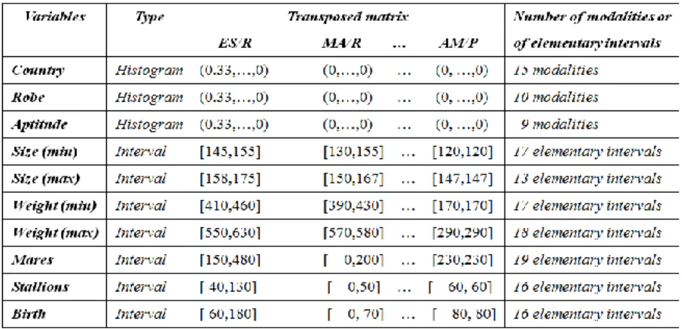
The histogram variables are Country (15 countries), Robe (10 categories) and

Aptitude (9 categories) and the interval variables are Height at the withers / Size (min), Height at the withers / Size (max), Weight (min), Weight (max), Mares, Stallions and Birth.

A brief description of the variables, by type, partial description over the set of statistical data units and number of modalities of each histogram variable or number of computed elementary intervals of each interval variable may be seen in the following table:

Table 4. Short description of Horse data set variables

Thus each variable (generalized column) gave place to a sub-table with a suitable number of columns corresponding to a set of modalities (for the first three modal variables) or a set of elementary intervals (for the seven last interval valued variables).

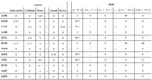
According to the previous table, the generalized data matrix describing the statistical data units (groups of horses), was split into ten sub-tables with twelve rows and a different number of columns. Table 5 partially illustrates the first and last sub-tables of the resulting generalized data matrix.

Table 5. Partial representation of the transformed data matrix for Horse data set

The two sub-tables represent, respectively, the first histogram variable Country (where the data units are described by their corresponding profiles, as they were displayed at the site) and the last interval variable Birth.

For the interval variable, Birth, each row of its sub-table contains the 16 ranges of the intersection intervals between each elementary interval and the interval assumed by Birth in the group of horses described by that row.

The hierarchical clustering models we used for classifying the twelve complex data units were based on either the weighted generalized affinity coefficient

) ' ,

(k k

a with equal weights, j1 p/ , or an associated coefficient related to the

probabilistic approach referred to above (see Section 2). Both coefficients were combined with several classical (single linkage-SL, complete linkage-CL, etc.) and probabilistic VL (V for Validity, L for Linkage) aggregation criteria in order to obtain hierarchical clustering models. Note that the VL methodology is a probabilistic clustering approach based on the cumulative distribution function of similarity coefficients under suitable reference hypothesis (e.g. Bacelar-Nicolau, 1987; Bacelar-Nicolau et al., 2009; Lerman, 1970, 1981, 2000), which may be combined either with classical or VL aggregation criteria.

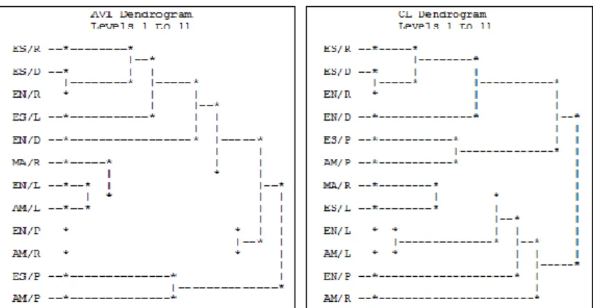
Two kinds of clustering typologies arise, one into four clusters and the other one into three clusters and a few singletons (from the corresponding numerical tables of similarities and aggregation criteria, as well as from appropriate quality/validity indexes to choose de most significant partitions). The dendrograms are represented in the following figure, where probabilistic and empirical hierarchical clustering approaches were respectively used:

Fig. 1. Dendrograms for hierarchical clustering models based on the global generalized affinity coefficient

The main four clusters, obtained with the hierarchical clustering models associated to the dendrogram shown on the left side of Figure 1, are {ES/R, ES/D, EN/R,

ES/L, EN/D}, {MA/R, EN/L, AM/L}, {EN/P, AM/R}, and {ES/P, AM/P}.

Alternatively, three main clusters emerge from the models giving the dendrogram on the right side, {ES/R, ES/D, EN/R, EN/D}, {ES/P, AM/P} and {MA/R, ES/L,

EN/L, AM/L}; then EN/P and AM/R join, one after the other, the third cluster,

instead of merging together.

The clusters {ES/R, ES/D, EN/R, EN/D}, {EN/L, AM/L} and {ES/P, AM/P} show to be consistent in the way they are built into the hierarchical clustering models we

have analyzed.

The following a priori classification into four classes was proposed for this data set: Racehorse (R)={ES/R, MA/R, EN/R, AM/R}, Leisure Horse (L)= {EN/L,

AM/L, ES/L}, Draft horse (D)={ES/D, EN/D} and Poney (P)={EN/P, ES/P, AM/P}. Therefore, looking at the consistent clusters indicated above, the first one

merges together the a priori draft horse and half racehorse classes. The second one is the a priori leisure horse class, without ES/L. The third one is the a priori poney class, without EN/P.

The horse data set was analyzed, among others, by De Carvalho and Souza (2010), with three non-hierarchical different algorithms. In their study, the clustering results also do not replicate the a priori classification. Besides, the authors obtain different partitions with different methods but they also find some consistent clusters, which in fact are the same consistent clusters we have listed above. Note that a hierarchical clustering model brings additional information on the way partitions are built.

4. Conclusions. Future developments

The three approaches described above for representing histograms, binary and interval valued variables lead to a comprehensive approach for measuring global proximity between complex data units (k, k’). The weighted generalized affinity coefficient holds for mixed data where those kinds of heterogeneous variables are present. In fact, it is a similarity coefficient defined for comparing distribution laws, gives the Ochiai and the generalized Ochiai coefficients for binary and interval variables, respectively, and may be represented by the same mathematical

expression for all three types of variables. Consequently, a unique algorithm works for those variable types.

Future developments include analyzing adaptive families of probabilistic clustering models and computational upgrading. Applications to real databases have mainly been developed in health and social sciences, education, economy and management.

Main References

1. Bacelar-Nicolau, H., On the distribution equivalence in cluster analysis, In Proceedings of the NATO ASI on Pattern Recognition Theory and Applications, Springer -Verlag, New York, pp. 73-79 (1987).

2. Bacelar-Nicolau, H., The Affinity Coefficient, In: Analysis of Symbolic Data: Exploratory Methods for Extracting Statistical Information from Complex Data, H.-H. Bock and E. Diday (Eds.), Series: Studies in Classification, Data Analysis, and Knowledge Organization, Springer-Verlag, Berlin, pp. 160-165 (2000).

3. Bacelar-Nicolau, H., On the Generalised Affinity Coefficient for Complex Data, Biocybernetics and Biomedical Engineering, vol. 22, no. 1, pp. 31-42 (2002).

4. Bacelar-Nicolau, H.; Nicolau, F.C.; Sousa, Á.; Bacelar-Nicolau, L., Measuring Similarity of Complex and Heterogeneous Data in Clustering of Large Data Sets, Biocybernetics and Biomedical Engineering, vol. 29, no. 2, pp. 9-18 (2009). 5. Bacelar-Nicolau, H.; Nicolau, F.C.; Sousa, Á.; Bacelar-Nicolau, L., Clustering Complex

Heterogeneous Data Using a Probabilistic Approach, In Proceedings of Stochastic Modeling Techniques and Data Analysis International Conference (SMTDA2010), pp. 85-93 (2010) (electronic publication).

6. Bock, H.-H. and Diday, E., Analysis of Symbolic Data: Exploratory Methods for Extracting Statistical Information from Complex Data, Series: Studies in Classification, Data Analysis, and Knowledge Organization, Springer-Verlag, Berlin (2000).

7. Chavent, M., De Carvalho, F.A.T., Lechevallier Y. and Verde, R., Trois nouvelles méthodes de classification automatique de données symboliques de type intervalle, Revue de Statistique Appliquée, vol. LI, no. 4, pp. 5-29 (2003)

8. De Carvalho, F. A. T. and Souza, R. M. C. R., Unsupervised pattern recognition models for mixed feature-type symbolic data, Pattern Recognition Letters 31, pp. 430-443 (2010).

9. Lerman, I. C., Sur l`Analyse des Données Préalable à une Classification Automatique (Proposition d’une Nouvelle Mesure de Similarité), Rev. Mathématiques et Sciences Humaines, vol. 32, no. 8, pp. 5-15 (1970).

10. Lerman, I. C., Classification et Analyse Ordinale des Données, Dunod, Paris (1981). 11. Lerman, I. C., Comparing Taxonomy Data, Rev. Mathématiques et Sciences Humaines,

38e année, no 150, pp. 37-51 (2000).

12. Matusita, K., On the Theory of Statistical Decision Functions, Ann. Instit. Stat. Math, vol. III, pp. 1-30 (1951).

13. Nicolau, F. C. and Bacelar-Nicolau, H., Nouvelles Méthodes d'Agrégation Basées sur la Fonction de Répartition, Collection Séminaires INRIA 1981, Classification Automatique et Perception par Ordinateur, Rocquencourt, pp. 45-60 (1982).

14. Nicolau, F.C. and Bacelar-Nicolau, H., Some Trends in the Classification of Variables, In: Hayashi, C., Ohsumi, N., Yajima, K., Tanaka, Y., Bock, H.-H., Baba, Y. (Eds.), Data Science, Classification, and Related Methods. Springer-Verlag, pp. 89-98 (1998). Address for correspondence

Helena Bacelar-Nicolau

Faculdade de Psicologia, LEAD; Universidade de Lisboa Alameda da Universidade 1649-013 Lisboa, Portugal