Computer-Vision-based surveillance of Intelligent Transportation Systems

(1)

F

ACULDADE DE

E

NGENHARIA DA

U

NIVERSIDADE DO

P

ORTO

Computer-Vision-based surveillance of

Intelligent Transportation Systems

João Neto

Mestrado Integrado em Engenharia Informática e Computação Supervisor: Rosaldo Rossetti, PhD

(2)

(3)

Computer-Vision-based surveillance of Intelligent

Transportation Systems

João Neto

(4)

(5)

Abstract

Traffic management is one of the most important and crucial tasks in modern cities, due to the increasing number of vehicles in the under dimensioned road networks. To aid in this task multiple solutions exist that simulate the networks behaviour taking for input data from traditional counting methods such as magnetic induction loops. These devices present flaws and are expensive to implement. With the decreasing cost of video cameras and the wide-spread use of computer vision, their use became a viable alternative to analyse traffic.

In this project we tackle the problem of automatic traffic surveillance using video cameras, developing a video analytics processor that will perform detection and classification tasks over gathered data. This processor was integrated in a solution under development that treats videos from multiple sources and provides computer vision as an on-line service.

A novel approach to the vehicle classification process is presented, based on the use of a fuzzy set. To illustrate the proposed approach, the detection and classification implemented were tested with different cameras in different scenarios, showing promising results.

(6)

(7)

Acknowledgements

Now that this period of my life is upon its dawn, it is time to thank everyone who accompanied me through this journey which has seen me grow both as an individual and as a professional. Without your support this adventure would not have been the same.

To the ρ7 Boyz, João Pereira, José Pinto, Henrique Ferrolho, Luís Reis and João Dias, as well as Sara Paiva and Beatriz Baldaia, the residents of Lab I120, thank you for all the good moments. To my parents and my brother for always being there for me, offering sage advice and true friendship. Thank you to my girlfriend Cátia Matos, who on a daily basis helped me face the toughest problems and overcome the greatest challenges.

To all my friends who showed a great degree of interest with this project, always ready to help, João Paiva, Jorge Wolfs, Sara Serra, Margarida Borges and Tomás Matos, thank you all.

I would also like thank my supervisor Prof. Dr. Rosaldo Rossetti for his guidance throughout the project as well as shedding some light into my professional life, and my second supervisor Diogo Santos for helping me take my first steps in the world of computer vision.

(8)

(9)

“The field is lost Everything is lost The black one has fallen from the sky and the towers in ruins lie The enemy is within, everywhere And with him the light, soon they will be here Go now, my lord, while there is time There are places below”

(10)

(11)

2.1.2 Our Challenge . . . 6 2.2 Image Treatment . . . 7 2.2.1 Blur . . . 7 2.2.2 Mathematical Morphology . . . 8 2.2.3 Shadow Removal . . . 11 2.3 Foreground Segmentation . . . 12 2.3.1 Background Subtraction . . . 12 2.3.2 Feature Tracking . . . 13 2.3.3 Edge Detection . . . 14 2.3.4 Object Based . . . 15 2.4 Object Detection . . . 15

2.4.1 Connected Component Labelling . . . 15

2.4.2 Convex Hull . . . 17

2.5 Object Classification . . . 18

2.5.1 Bounding Box Ratio Method . . . 18

2.5.2 Feature Clustering Method . . . 18

2.5.3 Artificial Neural Network with Histogram of Gradients . . . 19

2.6 Fuzzy Sets . . . 19 2.7 Traffic Analysis . . . 19 2.7.1 Highway Scenarios . . . 19 2.7.2 Urban Scenarios . . . 20 2.8 Summary . . . 21 3 Methodological Approach 23 3.1 Chosen Technology . . . 24 3.1.1 OpenCV . . . 24 3.1.2 JavaCV . . . 24 3.1.3 FFmpeg . . . 24 3.2 Techniques . . . 25

(12)

CONTENTS 3.2.1 Segmentation . . . 25 3.2.2 Object Detection . . . 26 3.2.3 Object Tracking . . . 27 3.2.4 Object Counting . . . 28 3.2.5 Object Classification . . . 28

3.2.6 Feature Point Tracking . . . 29

3.3 Summary . . . 29

4 Implementation and Results 31 4.1 Architecture . . . 31

4.2 Image Processors . . . 33

4.3 Multi-Feed Visualizer - Video Wall . . . 34

4.4 Image Segmentation . . . 37

4.5 Object Detection . . . 38

4.6 Object Tracking and Counting . . . 38

4.7 Classification . . . 40 4.8 Results . . . 43 4.8.1 Set-up 1 . . . 43 4.8.2 Set-up 2 . . . 43 4.8.3 Set-up 3 . . . 44 4.8.4 Set-up 4 . . . 44 4.8.5 Discussion . . . 45 4.9 Summary . . . 45

5 Conclusions and Future Work 47 5.1 Contributions . . . 47 5.2 Publications . . . 48 5.3 Future Work . . . 48 5.4 Final Remarks . . . 48 References 49 viii

(13)

List of Figures

2.1 Typical High-Way Traffic Scene . . . 6

2.2 Convolution Example [Lab17] . . . 7

2.3 Gaussian Function Variation with Sigma Value . . . 8

2.4 Morphology Operators typical structuring elements (5x5) a) Rectangular b) Cross c) Diamond d) Elliptical . . . 9

2.5 Result of the Erosion operator using a cross 3x3 kernel . . . 9

2.6 Result of the Dilation operator using a cross 3x3 kernel . . . 10

2.7 Result of the Opening operator using a cross 3x3 kernel . . . 10

2.8 Result of the Closing operator using a cross 3x3 kernel . . . 10

2.9 HSV color space components change due to shadows. Red arrows indicate a shadow passing on the point. Blue arrow indicates a vehicle passing [PMGT01] c [2001] IEEE . . . 11

2.10 Graphical example of the two-pass algorithm [Wik17] a) Original Image b) First Pass c) Second Pass d) Coloured Result . . . 16

2.11 Overview of the method as in [WLGC16] . . . 18

3.1 Project Planning . . . 23

3.2 Background Subtraction - Background Model . . . 25

3.3 Background Subtraction - Foreground Mask . . . 26

3.4 Object Life Cycle State Machine . . . 27

3.5 Object Tracking . . . 28

3.6 Multi-Feed Visualizer . . . 29

3.7 Object Classifier . . . 30

4.1 Manager Architecture . . . 31

4.2 Multi-Feed Visualizer 2x3 Example . . . 35

(14)

LIST OF FIGURES

(15)

List of Tables

4.1 Image Processors . . . 34

4.2 Results from Set-up 1 . . . 44

(16)

LIST OF TABLES

(17)

Abbreviations

2D Two Dimensions 3D Three Dimensions

ACM Association for Computing Machinery ADT Abstract Data Type

ANDF Architecture-Neutral Distribution Format API Application Programming Interface

ATON Autonomous Transportation Agents for On-scene Networked incident man-ager

BGSub Background Subtracter

CUDA Compute Unified Device Architecture FFmpeg Fast Forward Moving Pictures Expert Group HSV Hue, Saturation and Value

IEEE Institute of Electrical and Electronics Engineers ITS Intelligent Transport Systems

LIACC Laboratório de Inteligência Artificial e Ciência de Computadores MIT Massachusetts Institute of Technology

MRI Magnetic resonance imaging OpenCV Open Source Computer Vision RGB Red Green Blue

SAKBOT Statistical and Knowledge-BasedObject Tracker

YACCLAB Yet Another Connected Components Labelling Benchmark CAGR Compound Annual Growth Rate

(18)

(19)

Chapter 1

Introduction

1.1 Context

Traffic management in cities is a vast area as it studies the planning and control of the road network, with all the tasks associated with them. As the cities tend to evolve following the concept of smart cities, the management of how its people move is a prime area where the information technologies are being applied. With the increase in the number of vehicles using the roads [Nav00], this need to improve the methods of traffic management rise even more, and the development of multiple projects around the world around this issue comes as a confirmation of both it’s importance and the pertinence of the work being developed at LIACC in regards to this topic, the development of MasterLab, a dashboard for the management of traffic and transportation [ZRC14] [PRO10].

With the decreasing costs of cameras for video surveillance, the number of units installed around the world is rising, passing the 245 million mark in 2014 [Jen15], over 65% of that number being from Asia. With this number of cameras placed globally the amount of data being collected every day is too large to be humanly processed, and thus the need to create autonomous processors arises. The market for automatic analysis of video is expected to be worth 11.17 Billion USD by 2022 [Rep17], with the facial recognition area expected to have the highest CAGR (Compound Annual Growth Rate) due to the potential related to the security applications, even going as far as replacing airport checks in Australia by 2020 [Koz17].

The usage of computer vision to analyse traffic conditions has been around for some time now, with earlier works dating to 1990, such as the work by Rourke et. al [RBH90] where the advantages of using video analysis in this area are listed, as well as some issues that the community is still facing. Since then the field has been explored by many authors, applied to applications ranging from vehicle counting [CBMM98] [BMCM97] to incidents detection. Some work has been already developed at LIACC regarding this area of application of computer vision, namely an approach to use uncontrolled video streams found on web to perform traffic control in [LRB09].

Armis-Group is a company based in Porto that builds software in the areas of Information Management, Digital Sports and Intelligent Transport Systems. They are now developing two projects in the area of traffic analysis, Drive and Next [Adm17]. Drive is an innovative Traffic

(20)

Introduction

Management and Control solution, flexible and with an easy and fast set-up. Next is a complement to Drive that analyses, simulates and predicts traffic and events data. Due to the data simulation it is a valuable aid to the city operators decision making.

1.2 Project

The project for this dissertation was part of a collaboration between LIACC and Armis-Group. This collaboration aims to develop solutions in the field of Traffic Management, taking advantage of the laboratory’s resources and the company’s expertise and experience in the area. The objec-tive of the project was to design and develop a software module capable of analysing video and extracting relevant events on the roads as well as performing counting and basic classification of vehicles.

In the scope of the mentioned collaboration, LIACC developed a set of applications that form the "Video Server", a software package that aims to provide Computer Vision as a service, treating input streams as per user request. The analytics module developed during this dissertation work is part of its architecture.

The resulting module of the project can be used to analyse the traffic flow and to feed that in-formation to simulation systems such as described in [PRK11] [ARB15] [TARO10] [FRBR09]. Besides this, the project can be used as a complement to other counting mechanisms such as the ones presented in [SRM+16] and [BAR15].

1.3 Aim and Goals

The main goal of the dissertation is then to implement a solution that fits the needs of the project as stated above, detecting events in a short window of time to allow for fast response from the author-ities. This can be further broken down into more specific tasks to allow for a better understanding of the work ahead. The specific goals are as follows.

• To contribute for the effective integration of the implemented solution of this dissertation into their Armis Group commercial product;

• To implement solutions so as to perform the following tasks: Clear the image from noise and other unwanted features; Find objects of interest;

Classify detected objects; Detect relevant events.

• To test the implementation in a real scenarios. 2

(21)

Introduction

1.4 Dissertation Structure

This document is divided into four chapters. Chapter 2reviews the beginnings of computer vision, how it evolved and it’s applications, followed by an overview of basic image treatment techniques into more advanced ones, as well as presenting the more relevant work in the area of computer vision applied to traffic analysis. Chapter 3details the techniques applied during the development in a more practical approach. In Chapter 4the architecture of the implemented solution as well as the results of the work are presented and discussed. Finally, in Chapter 5conclusions of the work and the contributions of the dissertation are described, as well as where to take the project next.

(22)

Introduction

(23)

Chapter 2

Computer Vision and Traffic Analysis

-A literature review

2.1 History of Computer Vision

Computer vision appeared as an area of investigation around the mid 60’s at the MIT by Professor Larry Roberts, whose doctorate thesis focused on methods to extract 3D information from a 2D image [Hua96] in order to reconstruct entire scenes from the geometry gathered. This area is now considered by the ACM as a branch of artificial intelligence according to the 2012 ACM Computing Classification System [ACM12]. From this point onward scientists began applying the techniques developed in multiple fields.

The application of computer vision in the manufacturing industry was amongst the first ones to be explored. Due to the sheer number of robots working in the assembly lines of the factories that needed to be improved, as noted by Stout in 1980 [Sto80]. These robots were becoming outdated due to the lack of interaction with the environment. This meant that for a robot to work with a part in an assembly line it needed to be placed in a pre-determined position, and any deviation could mean that the line needed to be stopped. Michael Baird relates in [LB78] a computer vision system developed to inspect circuit chips rotation deviation in a welding base, indicating to the welder that the chip needed to be adjusted. Computer vision was also used as a tool to automatically analyse weather satellite images [BT73] and multidimensional medical images [Aya98], with applications being developed in these areas being now common in our daily life.

2.1.1 Computer Vision in Intelligent Transport Systems

Regarding intelligent transport systems (ITSs), the use of computer vision to aid in the analysis of traffic has been increasing in the last years due to the decreasing costs of hardware, both cameras, storage and processing power, as well as the growing knowledge to extract useful data from the video gathered. In contrast to the high installation and upkeep costs of other traffic control tools such as Inductive Loop Detectors and Microwave Vehicle Detectors, applying computer vision to handle these tasks is a profitable option for entities in charge of the analysis of this data.

(24)

Computer Vision and Traffic Analysis - A literature review

One of the first works applying computer vision to analyse traffic, which was published in 1984 [DW84] and detected and measured movement in a sequence of frames. Since then, multiple fields of study have been created, not only for the measuring of traffic, as explored in [LKR+16], [LRB09], [BVO11] and [HK12] where the authors evaluate methods to analyse traffic in urban environments, but also for the analysis of the environment around a self-driven vehicle, read-ing traffic signs usread-ing multiple approaches usread-ing convolutional neural networks [SS11] or using bag-of-visual-words [SLZ16], or to automatize the parking process as discussed in [HBJ+16]. Recently some studies have surfaced where the authors discuss the analysis of passenger numbers and behaviour inside vehicles, in order to enforce traffic laws [LBT17].

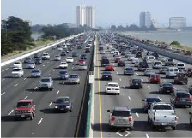
However our work upon this topic is focused on the aspect of traffic analysis. In order to understand what we need to accomplish, it is convenient to study what composes a typical traffic scene. Usually the scenes are viewed from a top-down perspective that places the cars against the road as background, as seen in Figure 2.1. The vehicles have a roughly regular rectangular shape when viewed from the top, with little variation when the camera is rotated, however their textures vary heavily, making it difficult for a detector to work based on the vehicles image representation [BP98]. However, depending on the camera position there can be object occlusion by other ob-jects or scene components, which makes it difficult to detect and track vehicles relying solely on subtraction based segmentation techniques.

Figure 2.1: Typical High-Way Traffic Scene

The scenes also have varying light according to the time of the day, and proposed solutions need to adapt to these changes as fast as possible, otherwise data might be lost. Other weather conditions can also interfere with the analysis, such as fog and rain, and need to be addressed when designing solutions.

2.1.2 Our Challenge

The "Analytics Server" module of the "Video Server" project had a list of requirements that needed to be addressed:

• Detect relevant events:

(25)

Wrong way driving; Fallen objects on the road; Prohibited zone entering;

Suspicious camera approximation

• Count and classify vehicles into light and heavy categories

The following sections of this document will explore the theoretical basis on which our solu-tion was built, aimed at tackling these specific points.

2.2 Image Treatment

This section will review some of the proposed methods to improve image quality before or during processing by removing noise, extracting unwanted features or enhancing relevant features for the processes involved.

2.2.1 Blur

In order to blur an image one needs to convolve it using a special kind of filter. The process of convolution in image processing consists in the application of a filter to every pixel of an image, returning a new image where each pixel is the result of the function to the pixel in the same position in the previous image. As we can see in Figure 2.2 the application of a 3*3 mask, where all 9 values have the value 1/9, results in a image where each pixel value equals the mean of itself and surrounding neighbours in the original image.

(26)

While this is the simplest blur processing we can apply to an image, there are more complex ones that yield better results. The one most often used in image processing is the Gaussian Blur, which uses a square filter with values calculated with the equation in 2.1from [SS01].

G(x, y) = 1 2πσ2e

−x2+y2

2σ 2 (2.1)

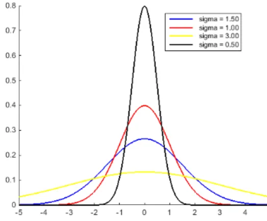
This equation returns a filter consisting of concentric circles that results in a smooth blurring of the images due to the application of the same power of blurring from equidistant pixels. The function can be tuned to the needs of the process through the σ value, returning a sharper or softer blur filter as seen in Figure 2.3.

Figure 2.3: Gaussian Function Variation with Sigma Value

This kind of filters have multiple uses in computer vision. Blurring an image removes the grain noise it contains, creating more even surfaces that ease the process of image processing, as well as making edges easier to detect with edge detection algorithms.

2.2.2 Mathematical Morphology

Mathematical Morphology is a set theory, offering solutions to multiple image processing prob-lems, where the sets are composed of tuples corresponding to the 2D coordinates of each pixel in the image. These sets identify the white or the black pixels in a binary image, depending on the convention adopted, or the intensity of the pixel in a grey-scale image [Dou92]. During this chapter we will consider that all images are binary and that the pixels to process are black in a white background. This theory provides a set of operators that can be used to detect convexity and connectivity of shapes in an image, enhancing features, detecting edges and removing noise.

The operators are defined by a structuring element, also known as kernel, a set of coordinates represented in a binary image, usually much smaller than the image to process. The centre of the kernel is not in the top left corner as in most images but rather in the geometrical centre, meaning that there some of the pixels have negative coordinates. The kernel shapes in Figure 2.4are the

(27)

ones typically used for most applications, but the process allows the user to design their own if needed.

Figure 2.4: Morphology Operators typical structuring elements (5x5) a) Rectangular b) Cross c) Diamond d) Elliptical

According to Gonzalez and Woods [GW92] an operator is defined by an image and a struc-turing element, and to run it the origin point of the element needs to be placed at every pixel of the image. At each of these locations a verification is done depending on the operation being performed and an output image is created using the independent output of these operations.

The two most basic operations are erosion and dilation, essential to morphological processing. The erosion operator translates the structuring element to every black pixel of the image and in each position checks if all the active pixels of the kernel match with black pixels in the image. If it is true then the returned pixel is black, otherwise it is white. An example of the usage of such an operator can be seen in Figure 2.5. These operators are mainly used to remove noise from binary images or to separate objects to enable individual labelling and counting.

Figure 2.5: Result of the Erosion operator using a cross 3x3 kernel

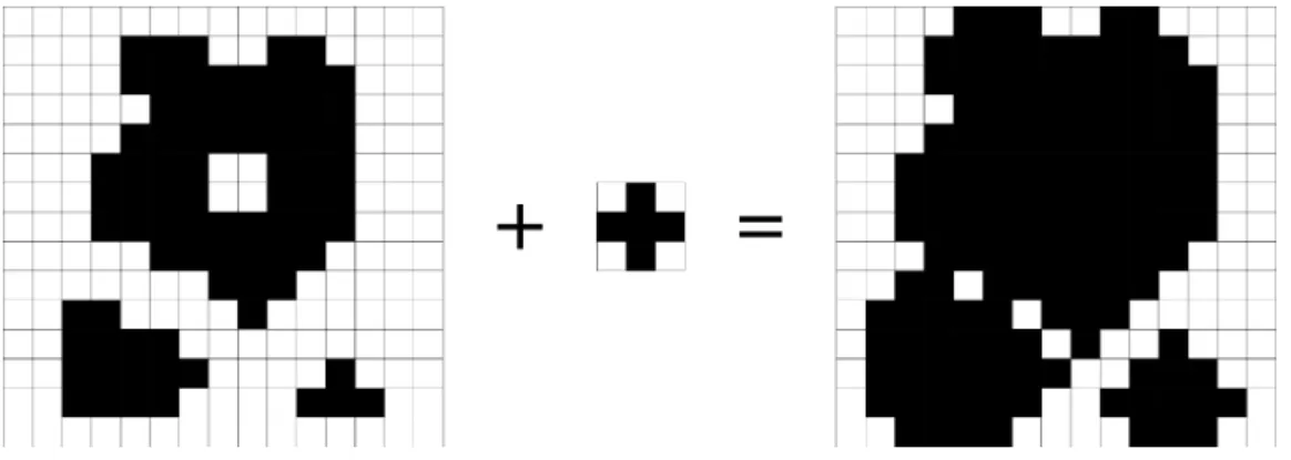
The dilation operator works by setting to black all the pixels that match the position of the translated kernel’s pixels, resulting in the closing of holes in the image and the enhancing of small features. Results can be seen in Figure 2.6. Using a non-symmetrical kernel the dilation will be directional, enabling the user to fine tune the process to their needs.

The dilation and erosion operators can be combined to form the opening and closing operators. An opening operator is formed by an erosion followed by a dilations using the same structuring

(28)

Figure 2.6: Result of the Dilation operator using a cross 3x3 kernel

element. This results in a less destructive erosion, preserving some of the image details as seen in Figure 2.7. The closing operator is formed by a dilation followed by an erosion and the results can be seen in Figure 2.8. It is commonly used to remove salt noise and to extract objects of a particular shape as long as they all share the same orientation [FPWW03].

Figure 2.7: Result of the Opening operator using a cross 3x3 kernel

Figure 2.8: Result of the Closing operator using a cross 3x3 kernel

(29)

2.2.3 Shadow Removal

Since shadows can be detected as foreground during the segmentation process, a process to re-move them is important in certain scenarios. We will now describe some of the more interesting proposed methods to perform this task in this section.

In [PMGT01] Prati et al. discussed how critical the shadow removal process is to traffic analysis, and they proceed to compare two ITS management systems, SAKBOT (Statistical and Knowledge-BasedObject Tracker) and ATON(Autonomous Transportation Agents for On-scene Networked incident manager), developed in Italy and the United States of America respectively.

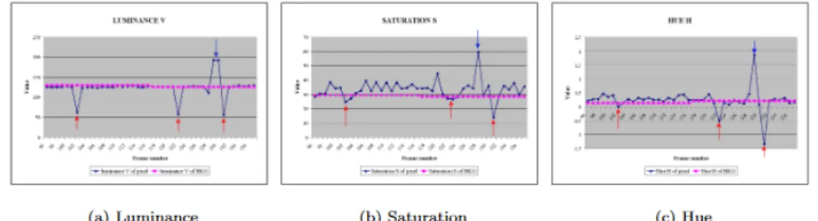
SAKBOT adopts a method presented in [CGPP00], which uses the chrominance information, converting pixel colours from RGB to HSV space, as it most closely relates to the human percep-tion of colour. The process then evaluates how the scene colours components change due to the passing of vehicles and shadows, as seen in Figure 2.9. From this we can extract that a shadow darkens a pixel and saturates its colour, and is the difference between an object point and a shadow point. The model then concludes that a point is considered as shadow if:

Figure 2.9: HSV color space components change due to shadows. Red arrows indicate a shadow passing on the point. Blue arrow indicates a vehicle passing [PMGT01] c [2001] IEEE

• The ratio between the luminance of the image and the background is between two thresholds (α and β )

• The difference between the saturation of the image and the background is below a threshold (τS)

• The absolute difference between the hue of the image and the background is below a thresh-old (τH)

The β value adjusts the tolerance to noise in the image to be considered as shadow and α takes into account the "power" of the shadow, how strong the light source is. τSand τH are considered

by the authors to be harder to assign, and thus assigned empirically. This method main advantage is it’s capability to detect moving shadows.

The method used by ATON is described in [MCKT00] and begins by identifying three separate sources of information to detect shadows and objects:

(30)

• Local information, the appearance of an individual pixel • Spatial information, objects and shadows are compact regions

• Temporal information, the location of shadows and objects can be predicted from previous frames

The local information can be used to create a background model, both the mean and variance of the colour for each pixel when shadowed and not shadowed. In the segmentation process the values in the image are compared to the mean value of the background and if significantly different it is assigned a probability to belong to the background, foreground or shadow. The probability values are 0.3, 0.4 and 0.4 respectively. In the next iterations the neighbour pixels probabilities are considered in order to take advantage of the spatial transformation. The iterative process stops when there are no relevant changes, usually after the third iteration. Morphological operators are then computed over the output of the process to close unwanted openings in the regions. ATON does not use temporal information as of the time of the publication of the work. This process can identify with near 90% accuracy shadows and object accuracy.

2.3 Foreground Segmentation

Image segmentation is the process through which an image is separated into its different regions according to the desired output, usually objects of interest. These regions are composed by pixels that have a common characteristic [SS01] dependant on the desired result. There are several ways one can accomplish an adequate segmentation of an image, and the most relevant ones to our purpose are described below.

2.3.1 Background Subtraction

Background Subtraction is a segmentation technique based on the analysis of the difference of consecutive frames and use that information to create a background model, a representation of what the image looks like without any moving objects present. Given the nature of the process, cameras must be static and although some research has been made to overcome this issue [LCC12] [SJK09] [ZY14], this is beyond the scope of the project, due to the requirements given.

There are however a number of different ways to implement the background subtraction devel-oped across the years with increasing segmentation accuracy and computational performance. Pic-cardi presented an overview of the most relevant ones in [Pic04], aiming to present each method’s strengths and weaknesses. From this work we can present a list of the algorithms considered for implementation in the project.

2.3.1.1 Frame Differencing

This is the simplest approach to the problem as it only considers two frames at a time, making it only work in certain scenarios where the speed of the objects and frame rate of the camera allow

(31)

it. In this model a pixel is considered as foreground if it satisfies the equation presented in 2.2, and since the only parametrizable value is the Threshold, the whole segmentation process is very sensitive to any changes in this value.

| f ramei− f ramei−1| >= T hreshold (2.2)

2.3.1.2 History Based Background Model

In order to make this segmentation method more robust, in the early 2000’s Velastin [LV01] and Cucchiara [CGPP03] proposed a mathematical model to take into consideration past frames when calculating the Background Model of the scene. The most simple version of the improved algorithm used a running average of the past frames as seen in 2.3. This eliminates the need to store the frames in memory as the new average can be calculated using the previous results.

BackgroundModeli+1= α ∗ Framei+ (1 − α) ∗ BackgroundModeli (2.3)

Instead of the running average one can use the median value of the last n frames, improving the method reaction to outlying values. In both however, the history can be just the n frames or a weighted average where recent frames have more weight. Both these methods cannot cope with intermittent changes on the background, such as moving leaves against a building facade, and to solve this problem a new approach was proposed, the Mixture of Gaussians which models each pixel according to a mixture of Gaussian distributions, usually 3 to 5, but in later research [Ziv04] a method was developed to calculate the number of distributions needed on a per pixel basis.

2.3.2 Feature Tracking

When the literature mentions features it is referring to interesting parts of the image that can be detected and matched in multiple different images of the same scene. The process of detecting these features is a basic step in many computer vision applications, as they allow for a broad comprehension of the scene being observed. These features can take the shape of:

• Edges - A boundary in an image (Further explored in the next section)

• Corners or Interest Points - Points in the image that have distinctive neighbourhood, making them good candidates for tracking

• Blobs or Regions of Interest - Connected areas of the image that share a property like colour or intensity

The OpenCV implementation of goodFeaturesToTrack is based on the work of Jianbo Shi et al. [ST94] that tackles the problem of selecting features that can be tracked consistently across

(32)

the scene, usually feature points that correspond to physical points in the scene. It does so by calculating a value they named dissimilarity that quantifies how much the feature appearance has changed between the first and the current frame. When this value grows past a certain threshold, the point is discarded and no longer tracked.

The two main improvements presented in this paper regarding this problem are the fact that the authors allow for both linear warping and translation regarding the image motion model, and the second being a numerically superior method for calculating the dissimilarity value when compared to existing work. The other main contribution is a new value to measure how good a feature is, beside the already common interest and cornerness. This value is the texturedness and is a result of the authors findings that features with good texture are more easily tracked.

2.3.3 Edge Detection

Detecting the edges in an image is an important step into the understanding of its contents, allow-ing segmentation based on surfaces and a spatial perception of the scene. The work presented by Marr and Hildreth [MH80] defines edges as part visual and part physical and proceeds to show that the two are interconnected. The first step of the proposed process is to calculate the zero-crossings of equation 2.4, the Laplacian of a two dimensional Gaussian applied to different scales of the image, which returns both the points of intensity change and the slopes of the function at that point.

∇2G(x, y) ∗ I(x, y) (2.4)

What the authors noted was that if an edge was detected at a certain scale it appears also at adjacent scales, which they called "spatial coincidence assumption". This theory can be reversed, if there is a convergence of edges on multiple scales there is a real physical edge, and based on this, if we find zero-crossings on neighbour scales, we can assume there is a real edge in that region. From here multiple implementations of the algorithm appeared, the most used one being presented below, the Canny Edge Detector using a Sobel filter. Although this was among the first implementations of an edge detector it is the most rigorously defined one and is still considered to be state of the art.

The Sobel filter is used to create an image that accentuates the edges of an original image. This process works by convolving two kernels with the image, one for the horizontal and the other for the vertical direction, that return the intesity change in that pixel for each one. The filters can be seen in 2.5as they were presented by Irwin Sobel [Sob89].

Gx=    +1 0 −1 +2 0 −2 +1 0 −1   , Gy=    +1 +2 +1 0 0 0 −1 −2 −1    (2.5) 14

(33)

Using Gx and Gy it is possible to retrieve the regions of the image that contain edges by

calculating the magnitude of the gradient vector as the square root of the sum of the squares of both components and thresholding these values. One of the features of this process is the ability to retrieve the direction of the edge from these values, using the inverse tangent operation.

The Canny Edge Detector uses the result of the Sobel filter as input and filters the most relevant edges as well as thinning them to 1-pixel wide lines. To accomplish this John Canny [Can86] used an optimization process comparing the value of the gradient magnitude to the one of the neighbour pixels along the direction returned by the Sobel filter, and keeping only the one with the largest value along the edge.

2.3.4 Object Based

Object Based segmentation relies on the a priori knowledge of the geometry of the objects we want to extract from the image. It is mainly used in medical applications such as in [SMG+93] where it is used to extract a model of the brain surface from MRI scans. To be able to use this approach to solve our issue of vehicle detection we would need detailed models of all the vehicles that can possibly pass through the scene we are analysing, which is not feasible, and thus this method was not further explored.

2.4 Object Detection

In this section we will analyse processes to detect objects of interest in images, a necessary step of any traffic surveillance system.

2.4.1 Connected Component Labelling

Connected component labelling is a process by which the subsets of connected components are labelled according to the user needs. We will explore some of the most common implementations and how they evolved over time.

The one-pass solution presented by Abubaker [AQIS07] is a fast and simple method to im-plement. It begins by labelling the first pixel of the image to 1, if it is a background pixel, skip to the next one, otherwise add it to a queue. While there are elements in the queue remove the one at the top and analyse its neighbours, if they are in the foreground add them to the queue with the current label. When there are no more elements in the queue increase the label number by one and proceed to the next unexplored pixel.

The two-pass solution presented by Shapiro et al. [SS01] uses the bi-dimensionality of the image data to transverse the pixels. The process, as the name implies, iterates over the image two times, the first time to assign temporary labels and the second to reassign these labels to the smallest ones available. It uses a neighbouring table to know what labels are adjacent to each other.

(34)

Perform a Raster Scan to analyse all the pixels For each pixel, if it belongs to the foreground

Get all its neighbours (four or eight depending on the connectivity assumed) Assign the smallest label from the neighbours

Add the the previous and the new label to the neighbouring table If there are no neighbour pixels add a new label

• Second pass

Perform a Raster Scan to analyse all the pixels

For each pixel assign the lowest label from the neighbouring table The process is illustrated in Figure 2.10.

Figure 2.10: Graphical example of the two-pass algorithm [Wik17] a) Original Image b) First Pass c) Second Pass d) Coloured Result

While these are the most basic solutions for the problem, a number of authors proposed en-hancements to improve their performance, the most prominent ones being the Contour Tracing Labelling by F. Chang et al. [CCL04], a method that uses contour tracing to identify internal and external contours of each component. These contours are then used to label the connected components when the image is traversed horizontally by counting the number of contours passed. The Hybrid Object Labelling presented by Herrero [MH07] presents a method that combines re-cursive and iterative analysis, finding unlabelled pixels and rere-cursively finding their neighbours until a labelled one is found, then proceeding to the assignment in the adjacent rows.

(35)

1 Input: Set of points in the plane

2 Output: List of vertices of the convex hull in clockwise order

3

4 Sort the points by their x-coordinate, creating a sequence p_{1}, p_{2}, ..., p_{n}

5

6 Put point p_{1} and p_{2} in a list called L_{upper}

7 for i=3 to n

8 Append p_{i} to L_{upper}

9 While L_{upper} has more than two points and the last three points don’t form a right turn

10 Delete the middle of the last three points from L_{upper}

11

12 Put points p_{n} and p_{n-1} in a list called L_{lower}

13 for i=n-2 down to n

14 Append p_{i} to L_{lower}

15 While L_{lower} has more than two points and the last three points don’t form a right turn

16 Delete the middle of the last three points from L_{lower}

17

18 Remove first and last point from L_{lower} to avoid duplication of the points where the upper and the lower hull meet

19 Append L_{lower} and L_{upper} and return that list

Listing 2.1: Convex Hull calculation

The implementation of OpenCV is based on the work of Grana et. al [GBC10]. It uses a new concept in this area that the authors describe as a single entry decision table and enhancing them to create the OR-decision tables that allow multiple equivalent decisions for the same conditions. The most convenient decision is selected by creating a decision tree, branching it whenever multiple decisions are possible. To improve the method performance the access to the image is made block-wise instead of the more usual pixel-block-wise manner. This is the chosen method for implementation in OpenCV due to it’s performance compared to other state of the art algorithms.

It is interesting to note the YACCLAB (Yet Another Connected Components Labelling Bench-mark) [GBBV16] project, a benchmark platform that allows researchers to compare the perfor-mance of their connected components labelling methods to the methods of other researchers. The novelty of this platform is the fact that it uses the authors implementations instead of their own, allowing the algorithms to perform exactly as intended, with all the tweaks and tricks.

2.4.2 Convex Hull

A convex hull is the smallest convex shape that encompasses all the points of the figure. This problem is usually solved in two or three dimensions, although some solutions can solve it for higher number of dimensions [Cha93]. In the field of computer vision however only the second and third dimension are needed.

An algorithm to calculate a convex hull from a set of points [dB08] can be seen in Listing

(36)

2.5 Object Classification

Some state-of-the-art approaches to the problem of object classification are explored in this sec-tion.

2.5.1 Bounding Box Ratio Method

To differentiate between pedestrians and vehicles Jiang Qianyin et al. [QGJX15] provided a method based on the analysis of the bounding box of each blob obtained by the background sub-traction method. They propose to compute the ratio of width and height of the rectangle and compare it to pre-calculated tabulated values. Using this approach they are able to distinguish pedestrians from small and large vehicles.

2.5.2 Feature Clustering Method

Figure 2.11: Overview of the method as in [WLGC16]

The method proposed by Shu Wang et al. in [WLGC16] categorizes three types of vehicles, compact, mid-sized and heavy-duty. It is described in some detail in figure2.11It works in four steps which will now be described.

In the first part a region of interest on a certain video is set manually where a pre-trained Fast Region-based Convolutional Neural Network is used to detect a vehicle in the image.

The second part is the feature extraction, and it performs it in two different forms. One of them uses a Deep Network to extract vehicle features and the other uses a pre-trained Extreme Learning Machine from which the authors obtain a weak label. This ELM is trained with cropped vehicle images and outputs in three different nodes representing the three different vehicle types. Both feature descriptors are fused together using a queue model which can be weighted according to specification.

The algorithm then takes these features and performs k-clustering on them, grouping them in three different clusters representing, once again, the three different vehicle types being analyzed.

After training the system we can use it to classify new samples, measuring the distance of the fused feature to the center of the clusters and choosing the one closer to the new point.

(37)

2.5.3 Artificial Neural Network with Histogram of Gradients

In their 2015 work [BG15] Sakan et al. use an ANN with HOG together with an analysis of the geometric features of to achieve better accuracy than the most used methods. A Histogram of Gradients is constructed by computing the gradients of small blocks of the image and grouping them into bins of 20 degrees each based on their orientation. Besides calculating the HOG, the authors also compute the length to height ratio of the bounding box of the vehicle as well as the ratio between the perimeter and the area. The ANN has as input the HOG and the geometric ratios calculated before and is trained with the backpropagation algorithm.

2.6 Fuzzy Sets

Fuzzy sets were introduced by L.A. Zadeh [Zad65] and Dieter Klaua [Kla67] in the mid 60’s. Although the work from Klaua is written in german, a very detailed analysis of his work can be found in a paper by Siegfried Gottwald [Got10].

Fuzzy sets are a class of sets where instead of each member belonging to a class like in regular sets, they have a degree of membership to each class ranging from zero to one. This degree is determined by the membership or characteristic function of the class it represents, and can also be seen as a truth value in certain applications.

Since their formulation, the use of these sets as spread to multiple areas: text processing [CBK00] where they are used to model linguistic modifiers taking into account relationships be-tween objects; vehicle safety [DSM12] in which they are used to build a fuzzy deterministic non controller type system that is able to indicate if a battery is on fire given a broad range of inputs; quality of life analysis [PB12] where they are used to analyse the effect of noise pollution caused by road traffic on the efficiency of human workers.

2.7 Traffic Analysis

The topic of traffic analysis using computer vision has been studied by multiple authors who tackled multiple problems. Since our solution is to be able to run on both highway and urban environments, both areas were studied.

2.7.1 Highway Scenarios

Highway scenes are more easily analysed due to the following attributes contributing to a con-trolled environment:

• Known object types in the scene, as we only have vehicles to analyse, with no pedestrians or other actors present;

• Cameras positioning is studied towards this type of application, meaning there is little to no occlusion of objects;

(38)

• The trajectory of the objects has little to no deviation.

In their work "Detection and classification of vehicles" [GMMP02] S. Gupte et al. present a method to replace the magnetic loop detectors with a vision-based video monitoring system. Their approach needs minimum scene-specific knowledge, an advantage that speeds up the set-up process. The vehicle tracking method proposed is based on a state machine where a region can belong to one of five different states:

• Update, when a region from the current frame matches exactly to a region in the previous frame;

• Merge, when multiple regions from the previous frame merge into a single one in the current frame;

• Split, when a single region from the previous frame split into multiple regions in the current frame;

• Disappear, when a region from the previous frame is not matched to any region from the current frame;

• Appear, when a region appears and is not near a recently disappeared region;

Using these five states they are able to track vehicles crossing the scene even if they are par-tially occluded behind other vehicles or scene features. They also present a classification technique that distinguishes cars from non-cars (vans, SUVs, semis and buses) based on the size of the re-gion using a fix threshold value. This was able to achieve a 70% classification success rate in a 20 minutes video.

Goo Jun et al. [JAG08] present a method for segmenting different vehicles inside the same region retrieved by the background subtracter. To do so they calculate a motion vector for each vehicle by tracking feature points across multiple frames and then clustering them based on their velocity.

2.7.2 Urban Scenarios

Urban scenes are harder to analyse due to the following attributes:

• Unknown object types in the scene, making it difficult to segment and classify them; • Cameras are positioned in low locations, creating a lot of occlusion between objects and

other objects, and objects and features in the scene; • Unexpected trajectories of the objects present in the scene;

• Objects may stop at any point and be classified as background by the segmentation process. 20

(39)

Buch et. al [BOV08] present a method to detect and classify vehicles in urban scenes that use 3D models whose projections are compared to the segmented regions. This method has a reported accuracy of 100% under sunny weather but this value declines when faced with foggy or rainy weather.

Hashmi et. al [HK12] propose an approach to gather statistics of intersection usage, analysing how many vehicles pass through the scene and also from where they come and where they exit. This evaluation is only possible using video, as the traditional methods of counting vehicles can-not establish a relationship between detections at different points of the intersection. This paper however can only deal with free-flowing traffic and has problems with stopped vehicles.

2.8 Summary

This chapter covered the basics of the field of computer vision and its multiple usages, reviewed basic concepts of image treatment, focusing on the ones that would be used during the development of the solution. When reading the work related to traffic analysis we detected a largely unsolved issue, related to the segmentation of stopped vehicles in urban scenes. This review was written taking into consideration that some of the readers may not be familiarized with the area, and thus contains overviews of some basic methodologies that are common in computer vision.

(40)

(41)

Chapter 3

Methodological Approach

As previously stated, the work done for this project consists of a module for the "Video Server" being developed by LIACC, that will perform all the required analytics of the video received. This chapter provides the details of the implementation of this module, developed during the dissertation semester between February and June 2017. Tasks performed involved designing an appropriate architecture, able to scale with the project, treating the images received from the video streams to detect events and extract information.

Figure 3.1: Project Planning

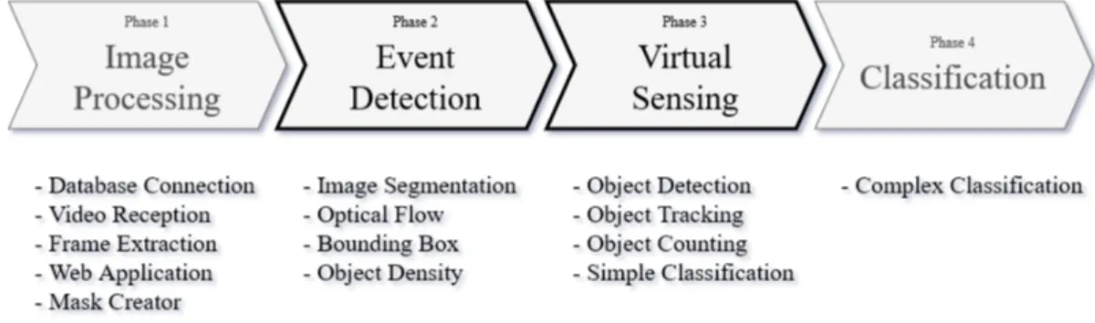
It is expected that this chapter provides some insight on how the theoretical backgrounds presented before were used during the project development, namely phase 2 and 3 of the planning presented in3.1. Phase 2 focused on the detection of relevant events to the traffic controller such as suspicious approximation to the camera, intrusion in prohibited areas, fallen objects on the road and wrong way travelling, while phase 3 aimed to count and classify vehicles in both urban and high-way scenarios.

(42)

Methodological Approach

3.1 Chosen Technology

In order to build this project we needed both a library of already implemented computer vision algorithms as well as a simple way to retrieve frames from both video streams and files. This section describes what were the chosen technologies including a brief description and why it was chosen.

3.1.1 OpenCV

OpenCV is a library composed of implementations of useful computer vision algorithms imple-mentation, widely used across the industry and academy. It has interfaces for multiple program-ming languages, like C++, Java and Python, but is natively written in C++ in order to take advan-tage of low level performance enhancements, as performance is an important factor in real time computer vision applications [Ope17a].

The library contains over 2500 algorithms ranging from the more basic image processing, such as filtering, morphology operators and geometric transformations, to more complex ones that are able to compare images, track features, follow camera movements and recognize faces, among others. Along with the image processing capabilities, OpenCV also ships with interfaces to stereo cameras such as Kinect that allow users to retrieve a cloud of 3D points and a depth map from the captured image. This was the chosen library as there existed already previous work at LIACC using it, which could be leveraged for this project.

3.1.2 JavaCV

JavaCV is a wrapper for OpenCV written in Java that works on top of the JavaCPP Presets, a project that provides Java interfaces for commonly used C++ libraries, such as OpenCV and FFm-peg, the ones we are using, as well as CUDA, ARToolKitPlus and others. It provides access to all the functionalities of OpenCV inside a Java environment, and was the chosen solution as there was already experience inside LIACC working with this technology.

Even though the code is written in Java and runs inside a Java Virtual Machine, the code from OpenCV is compiled from C/C++ and the memory of the objects created there is allocated in a separate thread. This made it impossible to rely on the garbage collector to do the memory management, and necessary to manually delete the native objects. Failure to address this issue causes the system to run out of memory and a subsequent program crash.

3.1.3 FFmpeg

FFmpeg is a framework that performs encoding, decoding, transcoding, streaming and filter oper-ations in all the well known video formats, across a large number of platforms. It is used in the "Video Server" to read streams from any format and restream them all to the same format. In the Analytic module it is used to grab the frames from both the video files and the streams using the same code, as shown in 3.1.

(43)

1 // videopath can be either a stream path or a file path

2 FFmpegFrameGrabber _frameGrabber = FFmpegFrameGrabber.createDefault(videopath);

3 Frame currentFrame = null;

4

5 while( (currentFrame = _frameGrabber.grabImage()) != null) {

6 // Use grabbed frame

7 }

Listing 3.1: FFmpegFrameGrabber usage example

3.2 Techniques

The following section presents a list of the techniques applied during the project, as they were described in Chapter 2, now diving into more technical details. Following this section a reader can implement a similar solution to the one presented in this document.

3.2.1 Segmentation

This section describes how the segmentation of the received images is performed, and how it returns a foreground mask representing the moving areas of the scene.

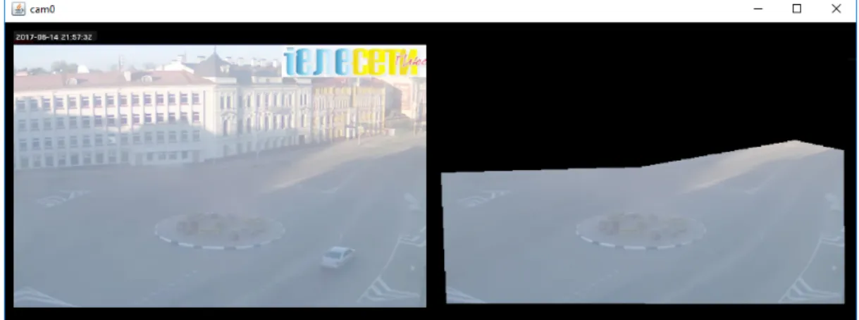
Figure 3.2: Background Subtraction - Background Model

In Figure 3.2we can see the original frame on the left and the calculated background model of the scene on the right. To achieve this result, the first step is to mask the obtained frame in order to prevent uninteresting regions of the image from being processed by the Background Subtracter. The masking process consists in placing a binary image, called a mask, over the original image and removing all the information where the mask has false values.

The application of the mask solves an issue where moving or changing regions of the image outside our area of interest would create unwanted artefacts, for example moving trees due to the wind blowing, or the issue that occurred in this scene, where a car passing would be reflected in the windows of the building.

(44)

The next step of the Segmentation process is to feed the masked frames into a Background Subtraction algorithm that will use them to update its internal representation of the scene. This project uses the OpenCV implementation of the Mixture of Gaussians algorithm that allows the user to tune:

• The number of past frames considered on the background calculation

• The threshold value from which a pixel is considered to be foreground, compared to the difference between its current value and the one from the background model

• The learning rate of the algorithm, how much each new frame influences the model

After updating the background model we can retrieve from the Background Subtracter its foreground mask, a rough representation that is calculated by subtracting the background model from the current image and thresholding it, thus returning only the pixels where the difference is significant enough.

Figure 3.3: Background Subtraction - Foreground Mask

As we can see in the middle image of Figure3.3the foreground mask from the Background Subtracter can have a lot of noise due to lighting conditions. To solve this issue two morphology filters are applied to the image: a squared erosion filter to remove the small speckles that appear in the mask; followed by a larger circular dilation filter to consolidate the positive regions of the mask, as the wind shield and windows of the vehicles are usually detected as background due to their dark colour and/or reflection of the environment.

3.2.2 Object Detection

This section describes how the information about the objects’ size and position are retrieved from the binary mask returned from the segmentation process.

OpenCV provides BlobDetector [Ope17b], a family of functions that retrieve information of blobs in an image. It works by thresholding the input into multiple binary images using a range of threshold values, grouping the connected white pixels at each one of these images in binary blobs and then merging those that are close enough to each other into larger blobs. This method allows users to filter returned blobs based on 3 properties:

(45)

• Area - The area of the region

• Circularity - Ratio between the area of the smallest involving circle and the area of the region • Convexity - Ratio between the are of the convex hull of the region and its area

• Inertia - Elongation of the region (0 for lines, 1 for circles)

This however does not work as intended for our input, an already binarized image where we just need to group the connected pixels. For this the project uses the OpenCV function connected-ComponentsWithStats, that retrieves the groups of connected pixels in a binary image along with their area, width, height and both the leftmost and topmost coordinate of the group’s bounding box. From this data we can create an ImageObject instance that will represent a moving object in the scene, using the regions with a size above a given threshold, in order to prevent detection of small objects or noise that got through the filtering process.

3.2.3 Object Tracking

In order for the solution to correctly analyse the objects of the scene it needs to track them during their lifetime, in other words, establish a relation between the objects identified on a frame with the objects identified in the next one. This is done by iterating through each one of the new objects and finding which existing object is closer to him. If the distance between them is smaller than the size of the existing object then they are matched.

Figure 3.4: Object Life Cycle State Machine

To enhance this mechanism a sub-set of the state machine presented by Jodoin et. al [JBS14] which allows us to model the life cycle of an object. As seen in Figure 3.4an object starts as an Hypothesis, and cannot be used for analytics while in this state. After being tracked for 5 frames it then changes its state to Normal, where it stays until no match can be found, either from leaving the scene or due to problems with the input frame. An object in this state remains for a maximum of 5 frames, after which it is deleted or until a new object is found in the vicinities of it’s last known position.

This technique relies on objects appearing close to their previous position in the next scene, and because the project was designed to run in high-way scenarios, where vehicles travel at high speeds, there was the need to improve it. The chosen solution was to follow a method used by Chris Dahms in his vehicle counting software [Dah17] that predicts an object next position by

(46)

calculating an weighted average of the previous inter-position deltas and summing it to its current position as shown in 3.1. NextPos= CurrentPos + 5

∑

i=1 (PosHist(i) − PosHist(i − 1)) ∗ (5 − i) (3.1)

In figure 3.5 we can see the result of the tracking process on the right most image. Each detected object is circled in a colour representing its current state in the state machine, blue for normal and red for lost, and shows the trail represents its path across the scene.

Figure 3.5: Object Tracking

3.2.4 Object Counting

This section will provide an overview of the environment created to support the development of the project, a flexible multi feed visualizer as seen in Figure 3.6. The top-left image shows the tracking process with the green zones indicating the virtual counting sensors. When a vehicle enters the sensor it is counted and classified. The middle top image shows the background model as calculated via the background subtracter explained in Section 3.2.1. The top right image and the bottom left one show the foreground mask before and after being processed by the morphological operators to remove the noise.

3.2.5 Object Classification

In order to classify the objects present in the scene into light or heavy vehicles a fuzzy set is used. This set is calculated at run time based on a mask drawn by the user via the web interface that roughly approximates the size of a light vehicle. The area of that mask (ALight) is used as a base

value to create the fuzzy set shown in figure3.7. This set has 2 series, one for light vehicles, drawn in blue, and one for heavy vehicles, drawn in red.

The blue series peaks at ALight, where we have 100% certainty that a matched object is a light

vehicle. The point immediate points are at 2/3*ALight, where the trust is 80% and at 4/3*ALight

where it drops to 60%. Any object with area below 1/2*ALightor above 2*ALightare considered to

have 0% chance to be light vehicles.

(47)

Figure 3.6: Multi-Feed Visualizer

The red series peaks at 2*ALight, and any object whose area is larger than this value is

consid-ered to be an heavy vehicle with 100% confidence. At the same time, any object whose area is smaller than 4/3*ALightis never considered to be an heavy vehicle, from where the certainty rises

to 80% at 5/3*ALight.

When an object is counted in one of the virtual sensors its area is passed to this classifier where an interpolation is calculated for each series, returning the certainty with which it belongs to each one of the classes. Using these values the process can distinguish classifications with certainty below and above a user specified threshold to be treated separately.

3.2.6 Feature Point Tracking

The need to track feature points stems from the fact that without them we rely wholly on the background subtraction to process the image. Using feature points we can extract and track details of the vehicles that would otherwise be lost due to the process only working with a binary mask.

We can use these points to distinguish vehicles grouped in a single binary region, as they are characterized by these features. This way, even if a vehicle stops for a long time and starts to be considered background we can use its tracked points to maintain the position of these stopped vehicles as they regain motion.

3.3 Summary

Although dealing with a framework with no proper documentation was a difficult challenge to overcome, the performance obtained from the native code was essential for the final result, as the software is now able to track objects in a busy scene faster than the camera’s capture rate, allowing us to process a video file in a shorter period of time than it’s length.

(48)

Figure 3.7: Object Classifier

(49)

Chapter 4

Implementation and Results

This section describes the architecture of the implemented solution as well as the results obtained during the testing phase of the project.

4.1 Architecture

Figure 4.1: Manager Architecture

The Analytics module was designed to comply both with the specifications imposed by our partner and with the characteristics of the modules already developed. The requirements are the following:

• Run uninterruptedly waiting for requests to be made; • Allow for video analysis with no significant delay;

(50)

Implementation and Results

• Process a large number of video inputs at the same time; • Receive input from streams or files;

• Specify which analysis are to be run on a specific video; • Use free-to-use or open-source tools;

• Allow for deployment scalability.

The application main thread runs an instance of the AnalyticsManager class that implements the Java Runnable interface. This thread will launch one CameraAnalyticsManager instance for each video to be analysed, be it from stream or from file, and keep track of each worker status. When a camera is disconnected from the server the corresponding thread is terminated. Likewise, when dealing with video from files, the thread is terminated when the all the analytics processors linked to that video are finished. The AnalyticsManager then enters a loop, pooling the database at a fixed interval, querying for cameras added to the system. When one is found, a new CameraAn-alyticsManager is launched, linked to that camera. The process can be seen in detail in Algorithm

4.1.

1 s t r i n g q u e r y = "SELECT ∗ FROM c a m e r a WHERE d o _ a l a r m s OR d o _ v i r t u a l _ s e n s o r s " ; 2 l i s t <Camera > c a m e r a s W i t h A n a l y t i c s = d a t a b a s e . q u e r y ( q u e r y ) ; 3 4 f o r e a c h c a m e r a i n c a m e r a s W i t h A n a l y t i c s 5 s t a r t N e w C a m e r a A n a l y t i c s M a n a g e r ( c a m e r a ) ; 6 end 7 8 w h i l e ( ! s t o p T h r e a d ) 9 n e w C a m e r a s W i t h A n a l y t i c s = d a t a b a s e . q u e r y ( q u e r y ) ; 10 f o r e a c h c a m e r a i n c a m e r a s W i t h A n a l y t i c s 11 i f ( ! c a m e r a . b e i n g A n a l y z e d ) 12 s t a r t N e w C a m e r a A n a l y t i c s M a n a g e r ( c a m e r a ) ; 13 end 14 end 15 w a i t ( 5 0 0 0 ) ; 16 end Algorithm 4.1: AnalyticsManager

The CameraAnalyticsManager is then responsible to query the database in order to find out what are the analytics the user wants to retrieve from the video through information that is stored in the camera table of the database. As of now there are three types of analytics that can be run over each input: Vehicle Tracking, Wrong-Way Travelling Detection and Suspicious Camera Approximation. Depending on the result of the query, a new thread is launched to perform each of the required analytics.

This process then starts a frame grabber that will convert each frame of the video into its representation in OpenCV and feed it to each Analyser through a queue. This enables each one

(51)

of these workers to run at his own pace and if one of them runs slower than the pace at which the frame grabber reads the images, it will simply queue them up and not slow down the remaining workers. The drawback of this solution is that it is theoretically possible to run out of memory to keep these frames, although this limit was not reached during the testing phase. The process can be perceived in more detail through the analysis of Algorithm 4.2.

1 2 c a m e r a A n a l y t i c s = g e t A n a l y t i c s F r o m D b ( c a m e r a ) ; 3 4 i f ( c a m e r a A n a l y t i c s . A l a r m A n a l y t i c s ) 5 i f ( c a m e r a A n a l y t i c s . WrongWay ) 6 launchWrongWayThread ( c a m e r a ) 7 end 8 i f ( c a m e r a A n a l y t i c s . C a m e r a A p r o x i m a t i o n ) 9 l a u n c h C a m e r a A p r o x i m a t i o n T h r e a d ( c a m e r a ) 10 end 11 end 12 13 i f ( c a m e r a A n a l y t i c s . V e h i c l e C o u n t i n g ) 14 l a u n c h O b j e c t T r a c k e r T h r e a d ( c a m e r a ) 15 end 16 17 w h i l e ( ! T h r e a d . i n t e r r u p t e d && ( c u r r e n t F r a m e = f r a m e G r a b b e r . g r a b I m a g e ( ) ) ! = n u l l ) 18 f o r e a c h c r e a t e d T h r e a d 19 c r e a t e d T h r e a d . f r a m e Q u e u e . p u t ( c u r r e n t F r a m e ) 20 end 21 end Algorithm 4.2: CameraAnalyticsManager

4.2 Image Processors

In order to streamline the use of some of the OpenCV functionalities a series of helper classes were created to help adjust the parameters of the algorithms during the development phase. These processors were implemented as subclasses of ImageProcessor, a superclass described in Listing

4.3.

The most relevant method of the described class is process(Mat original), the one that will be called in the code to use the processor. Each implementation of this abstract class will then contain an unique imageProcessorType that will allow us to distinguish the objects from each of them.

The ImageProcessor subclasses are listed in Table 4.1, along with their purpose and the pa-rameters that can be tweaked.

An addition to this functionality was made by introducing the concept of Image Processing Pipelines. This is a structure that groups multiple Image Processors into a single object, enabling us to run an image over all of the processors in a single call. The pipeline is created as an empty list and then the previously created processors are queued in the order they will be run.

(52)

1

2 public abstract class ImageProcessor {

3 protected final String imageProcessorType;

4

5 protected ImageProcessor(String imageProcessorType) {

6 this.imageProcessorType = imageProcessorType;

7 }

8

9 public abstract void process(Mat original);

10

11 public String getImageProcessorType() {

12 return imageProcessorType;

13 }

14 }

Listing 4.3: ImageProcessor class

Table 4.1: Image Processors

ImageProcessor Purpose Parameters

BackgroundSubtractor Perform background subtrac-tion over a sequence of frames

Learning rate of the background model, number of frames that are considered in the calculation, threshold for fore-ground consideration

ColorChanger Change colour scheme from black and white to colour and vice-versa

Direction of conversion

EdgeDetector Detect edges in an image First and Second threshold necessary for the Canny Operator

ImageResize Change the size of an image New size for the image ImageSmoother Perform a gaussian blurring

of the image

Size of the Gaussian filter

MaskProcessor Mask the input image Binary image containing the mask Morphology Apply a morphological

oper-ator to the input binary image

Which of the morphological operators to be run, the shape and size of the ker-nel

ShapePlacer Draw a rectangle, circle or convex polygon in an image

Which shape to draw, color and where to draw it

TextWriter Write text in an image Text to be written, font, size, color and lower-left coordinate

Thresholder Perform a thresholding oper-ation over the image

Value for the threshold operation

4.3 Multi-Feed Visualizer - Video Wall

The need for a multi feed visualizer arose during the development phase, as having the program open a new window for each feed that needed to be visualized was slowing down the development environment. The implemented solution overcomes this issue as it only needs a single window

(53)

Figure 4.2: Multi-Feed Visualizer 2x3 Example

and consequently, a single draw call.

The Multi-Feed Visualizer is implemented in the VideoWall class, shown in Listing 4.4. It takes as input the desired individual feed width and height output, the margin to be placed between the various feeds and the number of rows of columns that compose the feed visualization matrix. An example of the resulting structure can be seen in Figure 4.2. As for the implementation of the class, it can be seen in Listing 4.4and will now be detailed.

The VideoWall class relies heavily on the OpenCV concept of Region of Interest, a feature that allows for the selection of a rectangular area of an image and to display another image inside said rectangle. When an object of the VideoWall class is created, an empty image is created with the dimensions calculated as shown in Equation 4.1and 4.2.

Width= nCols ∗ videoWidth + (nCols + 1) ∗ margin (4.1)

Height= nRows + videoHeight + (nRows + 1) ∗ margin (4.2)

On this image we then calculate the regions of interest equal to the number of cells in the matrix at the specified positions. The show method then iterates through these regions and places a resized version of the input feed in each of the rectangles. These images also need to be converted to RGB colour space, as this is the one used by the output image.

Computer-Vision-based surveillance of Intelligent Transportation Systems

F

E

U

P

Computer-Vision-based surveillance of

Intelligent Transportation Systems

João Neto

Computer-Vision-based surveillance of Intelligent

Transportation Systems

João Neto

Abstract

Acknowledgements

Contents

List of Figures

List of Tables

Abbreviations

Chapter 1

Introduction

1.1

Context

1.2

Project

1.3

Aim and Goals

1.4

Dissertation Structure

Chapter 2

Computer Vision and Traffic Analysis

-A literature review

2.1

History of Computer Vision

2.2

Image Treatment

2.3

Foreground Segmentation

2.4

Object Detection

2.5

Object Classification

2.6

Fuzzy Sets

2.7

Traffic Analysis

2.8

Summary

Chapter 3

Methodological Approach

3.1

Chosen Technology

3.2

Techniques

∑

3.3

Summary

Chapter 4

Implementation and Results

4.1

Architecture

4.2

Image Processors

4.3

Multi-Feed Visualizer - Video Wall