Computer Sound Transformations Guided by Perceptually Motivated Features

(1)

Faculdade de Engenharia da Universidade do Porto

Computer Sound Transformations

Guided by Perceptually Motivated

Features

Nuno Figueiredo Pires

Master in Electrical and Computers Engineering

Supervisor: Professor Rui Luis Nogueira Penha

Second Supervisor: Dr. Gilberto Bernardes de Almeida

(2)

(3)

Resumo

Nesta disserta¸cão, apresentamos uma revalida¸cão de estudos feitos sobre descritores de som quente. A partir de um modelo existente, implementamos um algoritmo que define o warmth de um som harmónico monofónico. O algoritmo permite a produtores e a músicos, manipular o warmth de um áudio musical em tempo real (ou seja, performance ao vivo). O termo warmth cai numa categoria de conceitos de atributos musicais, tais como ”brilho”, ”aborrecido”, ”monótono”, os quais músicos e produtores musicais adoptam quando se referem a atributos t´ımbricos do som. Esta léxico musical é bastante relevante para a comunidade de peritos musicais. Porém, devido à sua natureza subjetiva, é dific´ıl definir um modelo matemático que nos permita manipular sons usando técnicas de processamento de sinal digital. Portanto, ao estarmos cientes da importância desta ferramenta de proces-samento, procuramos compreender os timbres que afetam tal atributo sónico informal e em segundo, codificá-la como um modelo matemático que possa ser utilizado para manipular o warmth the áudio musical em tempo real.

O descritor proposto manipula uma área de warmth calculada, que é baseada no tra-balho de D. Williams [1], onde o warmth é uma rela¸cão entre a energia dos três primeiros harmónicos e a energia do resto do espectro do sinal. Para este fim, nós regulamos as am-plitudes das componentes espectrais do áudio musical para moldá-los de acordo n´ıvel rel-ativo de warmth controlado pelo utilizador. Por outras palavras, permitimos ao utilizador reduzir ou aumentar a percentagem de warmthness dinamicamente do áudio musical de entrada mantendo a relativas varia¸cões, em tempo real.

Para primeiro tentarmos perceber de que forma é que o warmth num som instrumental é percepcionado, realizamos uma avalia¸cão perceptual que foi enviada para 128 pessoas com diferentes n´ıveis de proficiência musical.

Por forma a validar e avaliar a eficácia da nossa aplica¸cão, realizamos um segundo teste de escuta que contou com a participa¸cão de 51 indiv´ıduos.

Concluimos que, apesar de termos conseguido correlacionar o warmth com a centroid espectral, o algoritmo tem de ser melhorado pois a diminua¸cão do n´ıvel de warmth não é percet´ıvel.

(4)

(5)

Abstract

We present a revalidation of previous research done on description of warm sound. With an existing model, we elaborate an algorithm that defines the “warmth” of a monophonic harmonic sound. A twofold approach to the algorithm allows producers and musicians to not only measure this sound attribute but also manipulate it in real-time (i.e. a live performance).

The term warmth falls in a category of music audio attributes, such as bright, dull, flat, which expert musicians and music producers widely adopt to address timbral attributes of sound. This (semantic) musical jargon is highly relevant to the community of musical experts. Yet, due to its subjective nature, it’s hard to define mathematically, which would enable us to manipulate sounds using digital signal processing techniques. By being aware of the importance of such a processing tool, we strive here to first understand the timbral attributes which impact such an informal sonic attribute and second encode it as a mathematical model which can be used to manipulate the warmth of musical audio in real-time.

Based on the work of D. William and T. Brookes [1], the proposed warmth descriptor manipulates a certain ”Warmth Region”, where this ”warmth” is a relation between the energy of the first three harmonics and the energy of the remainder magnitude of the spectrum. To this end, we regulate the amplitudes of the spectral components of a musical audio, to shape them according to a relative user-controlled level of warmth. In other words, we allow the user to dynamically reduce or increase the percentage of warmthness in the musical audio input, while retaining the relative variability over time.

To first understand how warmth in instrumental sounds is perceived, we performed a perceptual evaluation, that was submitted to over 128 people of different levels of musical proficiency.

To validate and evaluate the effectiveness of the application we designed a second listening test that counted with the participation of 51 individuals.

We conclude that despite having a correlation between the warmth and the spectral centroid, the algorithm has to be improved as the decrease of warmth was not perceived.

(6)

(7)

Acknowledgment

I start by thanking my supervisor Professor Rui Penha for giving me the opportunity to work on this dissertation. I thank you for all the support and feedback given throughout this work. Ever since I discovered the class of Advanced Synthesis of Sound I decided that I would like to do my thesis with Professor Rui Penha, where I could join electrical an computer engineering and audio. I’d also like to thank my INESC-TEC supervisor Gilberto Bernardes for his tireless support, for always being available to teach me and correct my wrong doings and whose orientation was crucial for the completion of this thesis.

I thank all the elements of the Sound and Music Computing group for the meetings where we shared knowledge and brainstormed.

I’d also like to thank all my colleagues who accompanied me in this long journey, in particular to: Diogo “Souma” Sebe for his companionship and for all the delicacies you cooked at @Cisco’s; to the “owners” of the @Cisco’s Francisco “Cisco” Alpoim for all the moments during this endeavor and for helping reviewing this document; Diogo “Paquet´on” Dias for his friendship and support; Joni “7kratos” Gona¸calves for keeping us in check whenever we got together at @Cisco’s and for making me realize that FEUP really affects a person :). I’d also like to thank Alexandre “Russo” Pires, Joaquim “Quim” Ribeiro, Pedro “kun” Dinis and F´abio “Beer Guy” Vasconcelos for this final years and all laughable moments.

I’d like to give a special thanks to all my family that supported me all this years, specially to my godmother.

A very special and heartfelt thank you to my sister Ana for putting up with me all these years and for being my partner and friend. To my dear parents for always going further and beyond and doing the impossible for my well being and personal growth. Thank you mother for being my guardian angel and, despite the difficult moments,being there to guide me and help me overcome incoming obstacles. Thank you father for being my Superman and for supporting me and helping me all my life and for being my strength and guiding me during this past few months. Thank you both for allowing and helping me close this important chapter of my life and I hope to count on your advice and support from now on too.

Once again, thank you all!

Nuno Figueiredo Pires

(8)

(9)

“Failures, repeated failures, are finger posts on the road to achievement. One fails forward toward success.”

C. S. Lewis

(10)

(11)

List of Figures

2.1 Digital Audio Processing [9] . . . 4

2.2 Analog-to-Digital Conversion [10] . . . 5

2.3 Layers of audio analysis based on[16] . . . 7

2.4 Table of descriptor by G. Peeters [25] . . . 9

2.5 Architecture of Williams and Brookes’ sound warmth descriptor . . . 13

2.6 Definition of the Warmth Region . . . 13

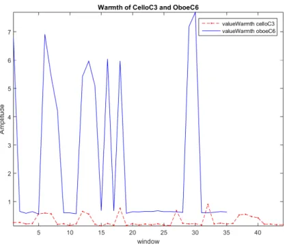
3.1 Responses of the first listening test with a graphical color code representation 17 3.2 Values of the spectral centroid of the violoncello C3 and oboe C6 sounds . . 20

3.3 Values of warmth of the violoncello C3 and oboe C6 sounds . . . 20

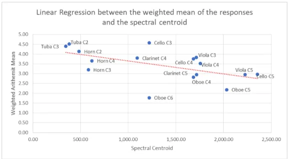
3.4 Linear regression between the weighted arithmetic mean evaluation and the spectral centroid of all instrumental sounds . . . 21

3.5 Linear regression between the weighted arithmetic mean evaluation and the warmth of all instrumental sounds . . . 21

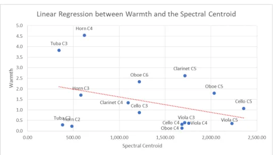
3.6 Linear regression between the warmth and the spectral centroid of all in-strumental sounds . . . 23

4.1 System Architecture . . . 26

4.2 First three harmonics of a Viola C4 sound . . . 27

4.3 Example of a window with overlap of four blocks . . . 27

4.4 Band-pass filter where only the values within the warmth region are allowed, and the rest is attenuated . . . 28

4.5 Reject-band filter where the amplitudes within the warmth region are at-tenuated . . . 28

5.1 Responses of the second listening test with a graphical color code represen-tation . . . 30

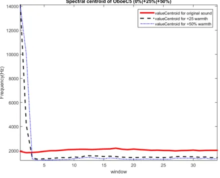
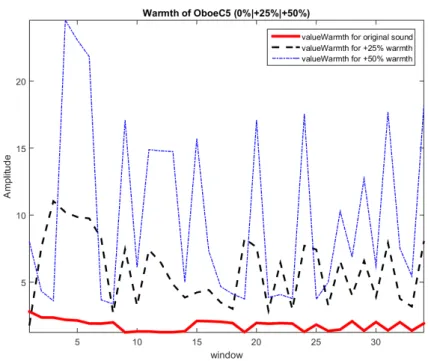
5.2 Values of the Spectral Centroid of the oboe C5 with 0%,+25% and +50% warmth . . . 34

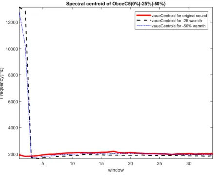
5.3 Values of the Spectral Centroid of the oboe C5 with 0%, -25% and -50% warmth . . . 35

5.4 Values of the Spectral Centroid of the oboe C5 with 0%,+25% and +50% warmth . . . 36

5.5 Values of the Spectral Centroid of the oboe C5 with 0%, -25% and -50% warmth . . . 36 A.1 Pure Data patch that receives the values of the Warmth Region and Spectral

Centroid of all frames and calculates the mean, media, and standard deviation 39 A.2 Pure Data patch that calculates the Warmth Region and the Spectral Centroid 40

(14)

A.3 Pure Data patch relative to the manipulation of the Warmth Region in

real-time . . . 41

A.4 Pure Data patch that performs the FFT of the signal, applies a band-pass filter and reject-band filter in order to get part of the signal related to the Warmth Region and the Remainder Magnitude, respectively, and allow the manipulation of the Warmth Region . . . 42

A.5 Pure Data patch that performs the manipulation of the warmth region based on a user input . . . 43

A.6 Pure Data patch relative to the creation of an array with the first three harmonics of the signal . . . 43

A.7 Listening Test 1 - instructions, in portuguese, of how to answer the first listening . . . 44

A.8 Listening Test 1 - instructions, in English, of how to answer the first listening 45 A.9 Listening Test 1 - characterization of the participant . . . 46

A.10 Listening Test 1 - example of question where the participant has to evaluate the sound according to the categories. This same type of question was done for all the sample chosen in Table 3.1. . . 47

A.11 Response chart for all three tuba examples . . . 47

A.12 Response chart for all three horn examples . . . 48

A.13 Response chart for all three clarinet examples . . . 48

A.14 Response chart for all three oboe examples . . . 49

A.15 Response chart for all three viola examples . . . 49

A.16 Response chart for all three violoncello examples . . . 50

A.17 Variation of the value of warmth in each audio file . . . 51

A.18 Mean median and standard deviation of warmth in the three tuba sound examples. The leftmost (at ’0’) values belong to the sound of tuba C2. The values at ’1’ belongs to the sound of tuba C3 and the rightmost (at ’2’) values belong to the sound of tuba C4 . . . 52

A.19 Variation of the value of the spectral centroid in each audio file . . . 52

A.20 Mean median and standard deviation of the spectral centroid in the three tuba sound examples. The leftmost (at ’0’) values belong to the of sound tuba C2. The values at ’1’ belongs to the sound of tuba C3 and the rightmost (at ’2’) values belong to the sound of tuba C4 . . . 53

A.22 Mean median and standard deviation of warmth in the three horn sound examples. The leftmost (at ’0’) values belong to the sound of horn C2. The values at ’1’ belongs to the sound of horn C3 and the rightmost (at ’2’) values belong to the sound of horn C4 . . . 54

A.23 Variation of the value of the spectral centroid in each audio file. . . 54

A.24 Mean median and standard deviation of the spectral centroid in the three horn sound examples. The leftmost (at ’0’) values belong to the of sound horn C2. The values at ’1’ belongs to the sound of horn C3 and the right-most (at ’2’) values belong to the of sound horn C4 . . . 55

A.26 Mean median and standard deviation of warmth in the three clarinet sound examples. The leftmost (at ’0’) values belong to the sound of clarinet C4. The values at ’1’ belongs to the sound of clarinet C5 and the rightmost (at ’2’) values belong to the sound of clarinet C6 . . . 56

(15)

LIST OF FIGURES xiii

A.28 Mean median and standard deviation of the spectral centroid in the three clarinet sound examples. The leftmost (at ’0’) values belong to the sound of clarinet C4. The values at ’1’ belongs to the sound of clarinet C5 and the rightmost (at ’2’) values belong to the sound of clarinet C6 . . . 57

A.30 Mean median and standard deviation of warmth in the three oboe sound examples. The leftmost (at ’0’) values belong to the sound of oboe C4. The values at ’1’ belongs to the sound of oboe C5 and the rightmost (at ’2’) values belong to the sound of oboe C6 . . . 58

A.32 Mean median and standard deviation of the spectral centroid in the three oboe sound examples. The leftmost (at ’0’) values belong to the sound of oboe C4. The values at ’1’ belongs to the sound of oboe C5 and the rightmost (at ’2’) values belong to the sound of oboe C6 . . . 59

A.34 Mean median and standard deviation of warmth in the three viola sound examples. The leftmost (at ’0’) values belong to the sound of viola C3. The values at ’1’ belongs to the sound of viola C4 and the rightmost (at ’2’) values belong to the sound of viola C5 . . . 60

A.36 Mean median and standard deviation of the spectral centroid in the three viola sound examples. The leftmost (at ’0’) values belong to the sound of viola C3. The values at ’1’ belongs to the sound of viola C4 and the rightmost (at ’2’) values belong to the sound of viola C5 . . . 61

A.38 Mean median and standard deviation of warmth in the three violoncello sound examples. The leftmost (at ’0’) values belong to the sound of violon-cello C3. The values at ’1’ belongs to the sound of violonviolon-cello C4 and the rightmost (at ’2’) values belong to the sound of violoncello C5 . . . 62

A.40 Mean median and standard deviation of the spectral centroid in the three violoncello sound examples. The leftmost (at ’0’) values belong to the sound of violoncello C3. The values at ’1’ belongs to the sound of violoncello C4 and the rightmost (at ’2’) values belong to the sound of violoncello C5 . . . 63

A.41 Listening Test 2 - instructions, in portuguese, of how to answer the first listening . . . 64

A.42 Listening Test 2 - instructions, in english, of how to answer the first listening 65 A.43 Listening Test 2 - characterization of the individual . . . 66

A.44 Listening Test 2 - example of question where the individual has to evaluate the modified sound taking into account the original audio file. Each modified sound could be equal to the original audio file, or with +-25% or +-50% warmth. This same type of question was done for all the audio file explained in Section5.1. . . 67

A.45 Chart of the responses for all four transformation of horn C4 . . . 68

A.46 Chart of the responses for all four transformation of clarinet C5 . . . 68

A.47 Chart of the responses for all four transformation of oboe C5 . . . 69

(16)

A.49 Chart of the responses for all four transformation of violoncello C5 . . . 70 A.50 Variation of the value of the spectral centroid of horn C4, when increased

the level of warmth by 25% and 50%, in each analysis audio file . . . 71 A.51 Variation of the value of the spectral centroid of horn C4, when decreased

the level of warmth by 25% and 50%, in each analysis audio file . . . 72 A.52 Mean, median and standard deviation of the spectral centroid of horn C4,

when increased the level of warmth by 25% and 50%, in each analysis audio file. The leftmost (at ’0’) values belong to the sound of horn C4 with no transformation. The values at ’1’ belongs to the sound of horn C4 with +25% warmth and the rightmost (at ’2’) values belong to the sound of horn C4 with +50% warmth . . . 73 A.53 Mean, median and standard deviation of horn C4 when decreased the level

of warmth by 25% and 50%. The leftmost (at ’0’) values belong to the sound of horn C4 with no transformation. The values at ’1’ belongs to the sound of horn C4 with -25% warmth and the rightmost (at ’2’) values belong to the sound of horn C4 with -50% warmth . . . 74 A.54 Variation of the value of warmth of horn C4, when increased the level of

warmth by 25% and 50%, in each analysis audio file . . . 75 A.55 Variation of the value of warmth of horn C4, when decreased the level of

warmth by 25% and 50%, in each analysis audio file . . . 75 A.56 Mean, median and standard deviation of the warmth of horn C4 when

increased the level of warmth by 25% and 50%. The leftmost (at ’0’) values belong to the sound of horn C4 with no transformation. The values at ’1’ belongs to the sound of horn C4 with +25% warmth and the rightmost (at ’2’) values belong to the sound of horn C4 with +50% warmth . . . 76 A.57 Mean, median and standard deviation of horn C4 when decreased the level

of warmth by 25% and 50%. The leftmost (at ’0’) values belong to the sound of horn C4 with no transformation. The values at ’1’ belongs to the sound of horn C4 with -25% warmth and the rightmost (at ’2’) values belong to the sound of horn C4 with -50% warmth . . . 77 A.58 Variation of the value of the spectral centroid of clarinet C5, when increased

the level of warmth by 25% and 50%, in each analysis audio file . . . 78 A.59 Variation of the value of the spectral centroid of clarinet C5, when decreased

the level of warmth by 25% and 50%, in each analysis audio file . . . 78 A.60 Mean, median and standard deviation of the spectral centroid of clarinet

C5, when increased the level of warmth by 25% and 50%, in each analysis audio file. The leftmost (at ’0’) values belong to the sound of clarinet C5 with no transformation. The values at ’1’ belongs to the sound of clarinet C5 with +25% warmth and the rightmost (at ’2’) values belong to the sound of clarinet C5 with +50% warmth . . . 79 A.61 Mean, median and standard deviation of clarinet C5 when decreased the

level of warmth by 25% and 50%. The leftmost (at ’0’) values belong to the sound of clarinet C5 with no transformation. The values at ’1’ belongs to the sound of clarinet C5 with -25% warmth and the rightmost (at ’2’) values belong to the sound of clarinet C5 with -50% warmth . . . 80 A.62 Variation of the value of warmth of clarinet C5, when increased the level of

(17)

LIST OF FIGURES xv

A.63 Variation of the value of warmth of clarinet C5, when decreased the level of warmth by 25% and 50%, in each analysis audio file . . . 81 A.64 Mean, median and standard deviation of the warmth of clarinet C5 when

increased the level of warmth by 25% and 50%. The leftmost (at ’0’) values belong to the sound of clarinet C5 with no transformation. The values at ’1’ belongs to the sound of clarinet C5 with +25% warmth and the rightmost (at ’2’) values belong to the sound of clarinet C5 with +50% warmth . . . . 82 A.65 Mean, median and standard deviation of clarinet C5 when decreased the

level of warmth by 25% and 50%. The leftmost (at ’0’) values belong to the sound of clarinet C5 with no transformation. The values at ’1’ belongs to the sound of clarinet C5 with -25% warmth and the rightmost (at ’2’) values belong to the sound of clarinet C5 with -50% warmth . . . 83 A.66 Variation of the value of the spectral centroid of oboe C5, when increased

the level of warmth by 25% and 50%, in each analysis audio file . . . 84 A.67 Variation of the value of the spectral centroid of oboe C5, when decreased

the level of warmth by 25% and 50%, in each analysis audio file . . . 84 A.68 Mean, median and standard deviation of the spectral centroid of oboe C5,

when increased the level of warmth by 25% and 50%, in each analysis audio file. The leftmost (at ’0’) values belong to the sound of oboe C5 with no transformation. The values at ’1’ belongs to the sound of oboe C5 with +25% warmth and the rightmost (at ’2’) values belong to the sound of oboe C5 with +50% warmth . . . 85 A.69 Mean, median and standard deviation of oboe C5 when decreased the level

of warmth by 25% and 50%. The leftmost (at ’0’) values belong to the sound of oboe C5 with no transformation. The values at ’1’ belongs to the sound of oboe C5 with -25% warmth and the rightmost (at ’2’) values belong to the sound of oboe C5 with -50% warmth . . . 86 A.70 Variation of the value of warmth of oboe C5, when increased the level of

warmth by 25% and 50%, in each analysis audio file . . . 87 A.71 Variation of the value of warmth of oboe C5, when decreased the level of

warmth by 25% and 50%, in each analysis audio file . . . 87 A.72 Mean, median and standard deviation of the warmth of oboe C5 when

increased the level of warmth by 25% and 50%. The leftmost (at ’0’) values belong to the sound of oboe C5 with no transformation. The values at ’1’ belongs to the sound of oboe C5 with +25% warmth and the rightmost (at ’2’) values belong to the sound of oboe C5 with +50% warmth . . . 88 A.73 Mean, median and standard deviation of oboe C5 when decreased the level

of warmth by 25% and 50%. The leftmost (at ’0’) values belong to the sound of oboe C5 with no transformation. The values at ’1’ belongs to the sound of oboe C5 with -25% warmth and the rightmost (at ’2’) values belong to the sound of oboe C5 with -50% warmth . . . 89 A.74 Variation of the value of the spectral centroid of viola C5, when increased

the level of warmth by 25% and 50%, in each analysis audio file . . . 90 A.75 Variation of the value of the spectral centroid of viola C5, when decreased

(18)

A.76 Mean, median and standard deviation of the spectral centroid of viola C5, when increased the level of warmth by 25% and 50%, in each analysis audio file. The leftmost (at ’0’) values belong to the sound of viola C5 with no transformation. The values at ’1’ belongs to the sound of viola C5 with +25% warmth and the rightmost (at ’2’) values belong to the sound of viola C5 with +50% warmth . . . 91 A.77 Mean, median and standard deviation of viola C5 when decreased the level

of warmth by 25% and 50%. The leftmost (at ’0’) values belong to the sound of viola C5 with no transformation. The values at ’1’ belongs to the sound of viola C5 with -25% warmth and the rightmost (at ’2’) values belong to the sound of viola C5 with -50% warmth . . . 92 A.78 Variation of the value of warmth of viola C5, when increased the level of

warmth by 25% and 50%, in each analysis audio file . . . 93 A.79 Variation of the value of warmth of viola C5, when decreased the level of

warmth by 25% and 50%, in each analysis audio file . . . 93 A.80 Mean, median and standard deviation of the warmth of viola C5 when

increased the level of warmth by 25% and 50%. The leftmost (at ’0’) values belong to the sound of viola C5 with no transformation. The values at ’1’ belongs to the sound of viola C5 with +25% warmth and the rightmost (at ’2’) values belong to the sound of viola C5 with +50% warmth . . . 94 A.81 Mean, median and standard deviation of viola C5 when decreased the level

of warmth by 25% and 50%. The leftmost (at ’0’) values belong to the sound of viola C5 with no transformation. The values at ’1’ belongs to the sound of viola C5 with -25% warmth and the rightmost (at ’2’) values belong to the sound of viola C5 with -50% warmth . . . 95 A.82 Variation of the value of the spectral centroid of violoncello C5, when

in-creased the level of warmth by 25% and 50%, in each analysis audio file . . 96 A.83 Variation of the value of the spectral centroid of violoncello C5, when

de-creased the level of warmth by 25% and 50%, in each analysis audio file . . 96 A.84 Mean, median and standard deviation of the spectral centroid of violoncello

C5, when increased the level of warmth by 25% and 50%, in each analysis audio file. The leftmost (at ’0’) values belong to the sound of violoncello C5 with no transformation. The values at ’1’ belongs to the sound of violoncello C5 with +25% warmth and the rightmost (at ’2’) values belong to the sound of violoncello C5 with +50% warmth . . . 97 A.85 Mean, median and standard deviation of violoncello C5 when decreased the

level of warmth by 25% and 50%. The leftmost (at ’0’) values belong to the sound of violoncello C5 with no transformation. The values at ’1’ belongs to the sound of violoncello C5 with -25% warmth and the rightmost (at ’2’) values belong to the sound of violoncello C5 with -50% warmth . . . 98 A.86 Variation of the value of warmth of violoncello C5, when increased the level

of warmth by 25% and 50%, in each analysis audio file . . . 99 A.87 Variation of the value of warmth of violoncello C5, when decreased the level

(19)

LIST OF FIGURES xvii

A.88 Mean, median and standard deviation of the warmth of violoncello C5 when increased the level of warmth by 25% and 50%. The leftmost (at ’0’) values belong to the sound of violoncello C5 with no transformation. The values at ’1’ belongs to the sound of violoncello C5 with +25% warmth and the rightmost (at ’2’) values belong to the sound of violoncello C5 with +50% warmth . . . 100 A.89 Mean, median and standard deviation of violoncello C5 when decreased the

level of warmth by 25% and 50%. The leftmost (at ’0’) values belong to the sound of violoncello C5 with no transformation. The values at ’1’ belongs to the sound of violoncello C5 with -25% warmth and the rightmost (at ’2’) values belong to the sound of violoncello C5 with -50% warmth . . . 101 A.90 Linear regression between the weighted arithmetic mean evaluation and the

spectral centroid of the sounds with increased level of warmth . . . 101 A.91 Linear regression between the weighted arithmetic mean evaluation and the

spectral centroid of the sounds with decreased level of warmth . . . 102 A.92 Linear regression between the weighted arithmetic mean evaluation and the

warmth of the sounds with increased level of warmth . . . 102 A.93 Linear regression between the weighted arithmetic mean evaluation and the

warmth of the sounds with decreased level of warmth . . . 103 A.94 Linear regression between the warmth and the spectral centroid of all

(20)

(21)

List of Tables

3.1 Chosen octaves for each instruments for the first listening test . . . 16 3.2 Results of the first listening test that aimed to evaluate how warmth in the

different instrumental sounds is perceived . . . 18 3.3 Weighted arithmetic mean, variance and standard deviation of the results

of the first listening test. The present Pearson correlation values result from a correlation between the values of warmth and the weighted mean values and also from a correlation between the values of the spectral centroid and the weighted mean values. . . 19 3.4 Values of warmth and spectral centroid of each instrumental sound. A

ratio between the warmth and the spectral centroid is also calculated. The present Pearson correlation value result of correlation between the values of warmth and the values of the spectral centroid . . . 22 4.1 Lowest Detectable Frequency according to the FFT window size,

consider-ing 44100Hz the samplconsider-ing rate . . . 26 5.1 Responses of the second listening test that aimed to evaluate the system . . 31 5.2 Weighted arithmetic mean, variance and standard deviation of the results of

the second listening test. The present Pearson correlation values result from a correlation between the values of warmth and the weighted mean values and also from a correlation between the values of the spectral centroid and the weighted mean values. . . 32 5.3 Calculation of the Warmth and Spectral Centroid of each instrumental

sounds that were modified according to a certain degree of warmth. It was also calculated the ratio between warmth and the centroid. The present Pearson correlation value result of the correlation between the values of warmth and the values of the spectral centroid. . . 33

(22)

(23)

Abbreviations and symbols

ADC Analog-to-Digital-Conversion DAC Digital-to-Analog-Conversion DSP Digital Signal Processing FFT Fast Fourier Transform

Hz Hertz - The unit of frequency of the International System MIR Music Information Retrieval

PCM Pulse-Code Modulation RM Remainder Magnitude

STFT Short-time Fourier Transform WR Warmth Region

(24)

(25)

Chapter 1

Introduction

1.1 Context

Today, audio processing enables composers and musicians to freely manipulate the char-acteristics of sound.

Traditionally, music experts refer to sound warmth according to two levels of granular-ity. The first one is rather broad and categorizes the timbre of different musical instruments from ‘cold’ to ‘warm’. For example, the low register of the clarinet tends to have a much warmer sound than the piccolo. Similarly, the horn has a much warmer sound than the trumpet. The second exists at a smaller scale and consists on the manipulations that expert musicians perform, shaping their instrument timbre according to different shades of warmth (e.g. in manipulating the point at which the bow hits the strings, a violinist can change drastically the sound warmth of the instrument - these techniques are referred to as sul tasto and sul ponticello). Music performers, composers and audio engineers have been wanting to manipulate qualities of timbre[2]. However, the last two decades marked a new scientific era in sound processing, having developed descriptors to extract attribute from the sound spectrum[3].

Music information retrieval(MIR)[4] is a growing field of research concerned with the extraction and inference of meaningful features from music (from the audio signal, symbolic representation), indexing of music using these features, and the development of different search and retrieval systems (for instance, content-based search, music recommendation systems, or user interfaces for browsing large music collections), as explained by Downie[5].

1.2 Motivation

Up to this day, the term warmth falls in a category of music audio attributes, such as bright, dull, flat, which expert musicians and music producers widely adopted to address timbral attributes of sound. This musical jargon is highly relevant to the community of musical experts.

(26)

Being still hard to define mathematically, creates an opportunity to further investi-gate and try to define an algorithm, a system, which would enable us to manipulate this subjective attribute of sound using digital signal processing techniques.

To a lesser extent, this dissertation aims to contribute to music perception by answering questions such as “Is this sound warm? How is warmth perceived? What is warmth?”. By the end of the dissertation it is hoped to get some clarifications on the matter.

1.3 Goals

The purpose of this dissertation is to expand upon previously published results and create a software to manipulate the warmth of sound that could be used worldwide in music production, in audio effects, music composition in general.

Towards this goal, we will start by reviewing the existing proposal of Williams et.al[1] and Antoine[6] and understand how the concept of warmth is perceived.

After this study, we design a listening test where the participants evaluate the level of warmth in several monophonic instrumental sounds.

Then, we develop, in a controlled environment, a descriptor based on additive synthesis. Accordingly, the definition of the descriptor will be redefined mainly regarding the output.

Ultimately, we generate a second listening test in order to evaluate the descriptor.

1.4 Document Structure

In Chapter 2 we review the state of the art of digital audio processing, introducing an overview of digital audio processing, music information and content-based description of musical audio signals. Later we review the existing work on warmth description in musical audio.

In Chapter3we present a perceptual evaluation of sound warmth , and results, which aims to evaluate how people perceive sound warmth.

In Chapter 4 we propose a system for manipulating the warmth in an audio file. We start by presenting an overview of our system, followed by a detailed explanation of its implementation.

In Chapter5we present the evaluation of our system. We detail and analyze the results of the listening test designed to evaluate the sounds that were transformed according to different levels of warmth.

(27)

Chapter 2

Overview of Digital Audio

Processing

In this chapter, we start with an overview of techniques and applications of Digital Signal Processing (DSP). After, we introduce the field of Music Information Retrieval, and its relevant techniques used to extract features from audio signals. Next, we present and detail the different levels of abstraction of audio description. The chapter concludes with the taxonomy of low-level layer of audio descriptors.

2.1 Digital Signal Processing

Digital Signal Processing[7] is the process of analysis and manipulation - applying mathe-matical and computational algorithms - of data from analog signals (such as sound, light or heat) that have been digitized or digitally generated signals. This includes a wide va-riety of technical tools such as: filtering; speech recognition; image enhancement; data compression; neural networks and more.

The use of DSP started around the ’70s, when digital computers first appeared and became one of the most powerful technologies that would shape science and engineering in the XXth century, across a large range of applications[8]:

• Communication Systems - modulation/demodulation, channel equalization, echo cancellation;

• Consumer electronics - perceptual coding of audio and video on DVDs, speech syn-thesis, speech recognition;

• Music - synthesized instruments, audio effects, noise cancellation;

• Medical Diagnostics - magnetic resonance and ultrasonic, imaging, computed to-mography, electroencephalography (EEG), electrocardiography (ECG), magnetoen-cephalography (MEG), automatic external defibrillator (AED), audiology;

(28)

• Geophysics - seismology, oil exploration;

• Astronomy - Very-long-baseline interferometry (VLBI), speckle interferometry;

• Experimental Physics - sensor-data evaluation;

• Aviation - radar, radio navigation;

• Security - steganography, digital watermarking, biometric identification, surveillance systems, signals intelligence, electronic warfare;

Sound and light are good examples of analog signals, which machines cannot compute. Therefore, a system is needed to convert analog signals to digital signals - a microphone regarding sound, and a digital camera if the signal is light.

In Figure2.1we show an example of analog and digital processing of sound. In analog processing the ear captures the sound waves and send them to the brain to process. In digital processing, the sound is captured by the microphone which is then converted from analog to digital and sent to an electronic device to be processed.

The Analog-to-Digital conversion system (ADC) performs the sampling of the signal’s amplitude at a sampling rate, Fs, followed by a quantization process, which converts to a Pulse-Code modulation (PCM). In Figure 2.2 we can see the process of converting an analog signal to digital format represented in a sequence of of 0’s and 1’s that machines can understand . When the signal is in digital format we are able to analyze, process and manipulate the signal.

To reconvert the signal from digital to analog it is used an Digital-to-Analog conversion (DAC) system that can convert the digital output signal to an analog output signal.

(29)

2.2 Music Information Retrieval 5

Figure 2.2: Analog-to-Digital Conversion [10]

2.2 Music Information Retrieval

At a time where technology tends towards ubiquitous computing, music is mainly accessed in digital format. We used to listen to music using the Walkman, Discman or even in a stereo system at home. Today music streaming is the trend, and there are a number of known services like Spotify1, Pandora2 and Deezer3 that have an enormous database from where the user can choose what to listen.

But this vast amount of digital audio available requires a deeper understanding of how to process audio signals, in particular how retrieving algorithms are formulated, to be able to extract information from the audio file to enhance user centered retrieval methods from these large archives.

1_{https://www.spotify.com/} 2_{https://www.pandora.com/} 3_{https://www.deezer.com/}

(30)

The field of research in MIR[11] gathers people with background on computer science and information retrieval, musicology and music theory, audio engineering and digital sig-nal processing, machine learning and psychology, working together to create and enhance toolboxes to better describe and extract relevant information from audio data[12].

MIR has several application domains[4] such as music retrieval, music recommendation, music playlist generation and music browsing interfaces. All these applications demand methods for retrieving information, for example audio identification or fingerprinting, where the goal is to retrieve or identify the same fragment of a given music recording with some robustness requirements. Another is query by humming and query by tapping, where the goal is to retrieve music from a given melodic or rhythmic input (in audio or symbolic format) which is described in terms of features and is compared to the documents in a music collection (i.e Shazam4)[13].

2.3 Content-based audio description

A lot of MIR research is based on human perception since the top-level ground-truth data mostly consists of human annotations[14]. The description of audio can be presented in an hierarchical structure, as shown by Herrera[15], from low-level to perceptual features (mid-level) and finally to a semantic description (high-level).

Descriptors are resources of digital audio processing that, from the temporal and spec-tral variation of the frequencies, represent the characteristics of the signal, which are useful for the creation of a taxonomy of the properties of the signal content.

2.3.1 Low-Level Descriptors

The literature in signal processing and speech processing documents a large amount of low-level audio features, either in the time domain (e.g. amplitude, zero-crossing rate, and autocorrelation coefficients) or in the frequency domain (e.g. spectral centroid, spectral skewness, and spectral flatness)[17]. They are computed from the digitized audio data by simple means and with very little computational effort in a straight or derivative fashion. Most low-level descriptors make little sense to humans, especially if one does not mas-ter statistical analysis and signal processing techniques, because the mas-terminology used to designate them denotes the mathematical operations on the signal representation.

2.3.2 Mid-Level Descriptors

As stated by Guti´errez[18], mid-level descriptors are used when it is necessary to carry-out operations which allow, after an analysis of the audio signal, to perform some generaliza-tion. This generalization can be a description of the data according to music theory, such as pitch, keys, meter, onsets, beats, harmonic complexity.

(31)

2.3 Content-based audio description 7

Figure 2.3: Layers of audio analysis based on[16]

A downside of this descriptor group is the time-consuming learning phase that most of the algorithms require[19].

2.3.3 High-Level Descriptors

High-level descriptors, also referred to as user-centered descriptors, express some categor-ical, subjective, or semantic attributes of the sound, such as mood and genre[20].

The computation of high-level descriptors involves some level of learning that is com-monly carried from user data (as is the case of mid-level descriptors). As an example, let us imagine a simplistic “mood” descriptor consisting of labels “happy” and “sad.” In order to automatically annotate unknown audio sources with such labels, it is necessary to initially create a computational model that distinguishes the two classes - happy and sad - by commonly relying on human annotations of audio tracks and machine learning algorithms; and then, one would be ready to compare a new track against the created model to infer its mood[19].

2.3.4 From Low-Level to Mid-Level to High-Level Descriptors

The jump from low- or mid-level descriptors to high-level descriptors requires bridging a semantic gap[15].

(32)

Audio descriptors are used in audio processing, to identify and manipulate sound char-acteristics that are perceived and qualified by the human ear. They are an essential instrument in MIR research that seek to systematize and model the qualitative sounds perception. The low-level audio descriptors are the basic components to analyze the sound as described in Figure2.4, created by Geoffrey Peeters.

For a better understanding, lets use gastronomy as an analogy where the sound is represented by the dish. We can say that low-level descriptors are proteins, lipids, carbo-hydrates. Mid-level descriptors represent the ingredients that make up the dish, like fish or meat, vegetable or spices. High-level descriptors correspond to the attributes used to identify the dish - if it is indian, mexican, chinese, japanese or italian - or if the dish is spicy, sour, bitter or blend.

Up next, we can see an approach to “recipes” of the attributes of the timber related to subjective perception of sound, such as:

Brightness is related to the spectral centroid[21]. The higher the spectral centroid, the brighter the sound.

Dullness is also related to the spectral centroid[22]. A low spectral centroid value indicates that the sound is dull.

Roughness is related to the iteration between partials within the critical bandwidth and also the energy above the 6th harmonic[23].

Breathiness It has been defined that breathiness is described comparing the funda-mental amplitude against noise content and the spectral slope[24]. The bigger the ratio between fundamental amplitude and the noise content, the breathier the sound.

2.4 Taxonomy of low-level audio descriptors

A system for the extraction of audio descriptors is usually organized according to the taxon-omy of the descriptors. We can distinguish three main properties of an audio descriptor[25]: temporal energy envelope, spectrum shape and sinusoidal harmonic partials, or just har-monic. The temporal energy envelope can be defined as a global descriptor and the autocorrelation coefficients, zero-crossing rate, spectrum shape and the harmonic defined as time-varying descriptors.

2.4.1 Temporal Energy Envelope

The temporal energy envelope can be illustrated by several descriptors, such as: attack, decay, sustain, log-attack time, temporal centroid, frequency and amplitude. This are used to know the sound’s characteristics and behavior along the domain of time.

(33)

2.4 Taxonomy of low-level audio descriptors 9

Figure 2.4: Table of descriptor by G. Peeters [25]

• Temporal Centroid (TC) - is the temporal center of gravity of the energy envelope. It is used to analyze percussive sounds.[25]

TC= n2 ∑ n=n1 tn· en ∑ n en (2.1)

Where: n1 and n2 are the first and last values of n, respectively, so that en is above

15% of its maximum value.

2.4.2 Spectral Features

The spectrum shape can be described by several descriptors, such as: autocorrelation, zero crossing rate, spectral centroid, spectral kurtosis, spectral skewness, spectral spread and frame energy. The spectral descriptors extracted are the following [26] [25]:

(34)

• Spectral Centroid corresponds to the spectral center of gravity of the spectrum and is known to be connected to the perceptual feature brightness:

SC= K ∑ k=1 fk· ak K ∑ k=1 ak fk= i · samplerate FFTwindowSize (2.2) Where:

K, is half of the FFT window size;

k, is the bin index;

ak, is the magnitude of the bin k

fk, is the frequency of the bin k, in Hertz.

• Spectral Spread (SS), also known as spectral standard-deviation, measures the variance of the spectral centroid:

SS= s K

∑

k=1 ( fk− SC)2· pk pk= ak K ∑ k=1 ak (2.3)

Where pkrepresents the normalized value of the magnitude of the Short-time Fourier

Transform (STFT).

• Spectral Skewness gives a measure of the asymmetry of the spectrum around its center of gravity: SSk= K ∑ k=1 ( fk− SC)3· pk SS3 (2.4)

• Spectral Kurtosis (SK) allows a measure of spectrum flatness around its centroid:

SK= K ∑ k=1 ( fk− SC)4· pk SS4 (2.5)

(35)

2.4 Taxonomy of low-level audio descriptors 11 • Spectral Slope slope= n K ∑ k=1 fk· ak− ( K ∑ k=1 fk· K ∑ k=1 ak) K ∑ k=1 ak· (K K ∑ k=1 f_k2− (∑K k=1 fk)2) (2.6)

• Spectral Decrease (SD) represents the magnitude decrease of the spectrum. It was proposed by Krimphoff[27] in his perceptual studies:

SD= K ∑ k=2 ak− a1 k− 1 K ∑ k=2 ak (2.7)

• Spectral Roll-off (SR) is defined as the frequency fc below which 95% of the

signal energy is contained. This feature was proposed by Sheirer et.al[28], where x represents the roll-off point:

SR= fc

∑

f=0 a2_f = x · Fn

∑

f=0 a2_f (2.8)

Where Fn is the Nyquist frequency.

2.4.3 Sinusoidal Harmonic Partials

The harmonic can be described by a group of descriptors, such as: harmonic energy, noise energy, noisiness, fundamental frequency, tristimulus and harmonic spectral deviation[25]. • Harmonic energy is the energy of the signal corresponding to the harmonic partial:

EH= H

∑

h=1

a2_h (2.9)

• Noise energy is the energy of signal not containing the harmonic partials:

EN= ET− EH

ET=

∑

i

a2_i (2.10)

• Noisiness is the ratio of the noise energy to the total energy:

noisiness=EN ET

(36)

• Tristimulus was first introduced by Pollard et.al[29] as a timbral equivalent to color attribute in vision. It consists of three different energy ratios, allowing a good description of the first harmonics of the spectrum:

T1 = a1 H ∑ h=1 ah T2 =a2+ a3+ a4 H ∑ h=1 ah T3 = H ∑ h=5 ah H ∑ h=1 ah (2.12)

Both the spectrum shape and the sinusoidal harmonic partial are used to analyze the audio along the frequency domain.

2.5 Description of Sound Warmth

2.5.1 Williams and Brookes’ Metric

The study of the warmth of a sound came following their previous studies on brightness and softness[30][31][1]. In their research, they selected warmth as the third timbral at-tribute because it has a certain degree of acoustic overlap with the perceptual feature brightness[32]. It has been shown that warmth has a correlation with spectral slope, spectral centroid and a relation between the energy of the first three harmonics and the remainder of the signal[33].

During the development of the hybrid timbre morpher[1], Williams and Brookes first extracts and interpolates the warmth, followed by a compensation of the acoustic overlap between all three perceptual features (brightness, softness and warmth). In Figure2.5we show a block diagram as an overview of their study.

2.5.1.1 Warmth Region

The warmth region is the area contemplating the energy between the signal’s fundamental up to 3.5 times this frequency. When in the presence of a harmonic signal this area would encompass the first three harmonics. In the case of a signal containing inharmonic partials and/or noise component, the energy in this area is intended to perform a similar timbral role to that of the first three harmonics.

WarmthRegion=W R

(37)

2.5 Description of Sound Warmth 13

Figure 2.5: Architecture of Williams and Brookes’ sound warmth descriptor

W R= 3.5

∑

f=1 af (2.14) RM= FM −W R =

_∑

f af ,where f ∈ R+0 \ [1 3.5] (2.15)

Figure 2.6: Definition of the Warmth Region

2.5.2 Aur´elian’s Metric

Aur´elian followed the study of William and Brookes[1] by adding a listening test us-ing samples of several instruments in terms of timbral characteristics such as brightness, breathiness, roughness, dullness and warmth[6].

(38)

The results for the first four perceptual features showed strong correlation between the participant’s responses and the classification system ratings[6]. However, the same cannot be said for warmth, as the results felt short and inconclusive.

Given the lack of results and more in-depth information regarding his approach for the analysis of warmth in sound, we designed an experiment which aims at evaluating the perceptual basis of the attributes considered in both metrics, which we detail at length in the following Chapter.

(39)

Chapter 3

Accessing the perceptual

manifestation of sound warmth

Previously, we reviewed the metrics that have been proposed in related literature to gauge the warmth of a sound. Given the limitations, we compare the perception of warmth in sound with the existing metrics, we conducted an online listening experiment of a set of instrumental sounds.

This chapter details an experiment design followed by exposure of the results and ends with the analysis of the instrumental sounds. In other words, we present and comment on the values of warmth and spectral centroid of the instrumental sounds used on the listening test.

3.1 Perceptual Evaluation

3.1.1 Listening Test

In order to design this listening test1, we used the IRCAM’s SOL database of acoustic instruments. In this database we can find audio samples from almost all families of in-struments (with the exception of percussion) which cover a wide spectral range, roughly from the lowest octave (e.g A123) to the highest octave (e.g A8).

Due to the vast number of samples, with their unique timbral richness, and taking into account the extension of the listening test[34], we created a data set consisting of 18 acoustic instrumental sounds - two instruments for each family of instruments and three octaves for each instrument - with variable duration, ranging from 2 to 8 seconds. The criteria for selecting these samples was that all instruments had to have the central C (Do)

1_{The listening test is available at}_{http://npires91.polldaddy.com/s/listening-test-1} 2_{Music notation using the alphabet to represent musical notes, from A (La) to G(Sol)}

3_{Music notation, using numbers, to represent the octave of the musical note (commonly present in a} piano keyboard), where 1 represents 1st (lowest) octave and 8 represents the 8th (highest) octave

(40)

sound as a common audio sample, which can be seen in Table 3.1. The test can be found in AppendixA.2.

Participants were asked to rate on a 7-point Likert scale (1-7) the level of warmth of the instrumental sounds, where 1 corresponds to not warm at all and 7 to completely warm. They were asked to listen - using high quality headphones - to the entire duration of the sound before rating it. To prevent response bias introduced by order effects, the musical examples were presented in a random order. To submit their ratings and complete the listening test, the participants were asked to rate all sound examples.

``_`` ``_`` ``_`` `` Instruments Octaves C1 C2 C3 C4 C5 C6 C7 Tuba X X X Horn X X X Clarinet X X X Oboe X X X Viola X X X Violoncello X X X

Table 3.1: Chosen octaves for each instruments for the first listening test

3.1.2 Results

The size of the perceptual study sample was of 128 individuals, with the following profiles:

• Age - from 17 to 45 years old

• Gender - 67% male and 33% female

• Musical proficiency - 13% with high expertise in music production, creation and performance; 45% with some expertise and 42% with no expertise;

To examine the results of the listening test we show the number of responses per musical example for each level of warmth.

Figure3.1shows the results using color system, in column “Octave” the gradient from turquoise to dark orange, where the first represents a higher and colder pitch and the latter represents a lower and warmer pitch. We also highlight the responses, for each audio sample, where dark brown represents the level of warmth with most responses and light brown with level of warmth with second most responses. The same results can be seen in Table 3.2.

Taking a closer look at the results for the tuba and horn, we can see that the responses concentrated in the same level of warmth, as the majority answered “Moderately warm” for the distinct sounds.

(41)

3.2 Analysis of the instrumental sounds 17

Figure 3.1: Responses of the first listening test with a graphical color code representation

On the other hand, the string family instruments (viola and violoncello) were evaluated as expected as we can see a step-like distribution in their responses. For lower octaves, they were evaluated with a higher level of warmth.

In the responses for the clarinet we can see a step-like distribution, similar to the strings family responses. For the oboe, the results of the sounds example C5 and C6 were evaluated as expected, but for the C4 participants were divided which resulted in evaluation both slightly, very slightly and moderately warm.

In order to know which sound was evaluated as the warmest, and least warm, we calculated the weighted arithmetic mean of the results, where each evaluation had a weight from 1 to 7 (the same as the Likert scale). After examining Table 3.3 we conclude that the sound of the violoncello C3 was the warmest sound and, on the other hand, the sound of the oboe C6 was the least warm of the data set.

3.2 Analysis of the instrumental sounds

For the purpose of knowing if there is a correlation between the warmth and spectral centroid of the musical examples and the results from the listening test, we created a pure data patch (Figure A.2an A.1) that calculates the warmth and spectral centroid of each analysis window for each instrumental sound. It also calculates the mean and standard deviation of the values of warmth and spectral centroid and also a ratio between warmth and the centroid, which are presented in Table 3.4. All the results were gathered and analyzed using a Matlab script.

(42)

Range 1 2 3 4 5 6 7

Instruments Octave Not warm Very slightly warm Slightly warm Moderately warm Very warm Extremely warm Completely warm Tuba C2 4 13 17 30 24 23 17 C3 6 12 12 33 34 22 9 C4 7 12 25 44 19 16 5 Horn C2 0 10 16 28 25 21 14 C3 7 11 28 35 20 7 2 C4 3 15 16 28 21 19 8 Clarinet C4 4 19 31 38 19 15 2 C5 15 42 27 29 11 2 2 C6 66 34 13 7 5 2 1 Oboe C4 17 37 35 31 7 1 0 C5 38 52 21 12 4 1 0 C6 74 32 9 7 4 0 2 Viola C3 6 16 26 41 26 11 2 C4 9 21 40 39 21 2 1 C5 18 39 26 28 12 4 1 Cello C3 3 7 16 31 42 16 13 C4 4 20 32 37 21 10 4 C5 13 48 24 25 13 2 3

Table 3.2: Results of the first listening test that aimed to evaluate how warmth in the different instrumental sounds is perceived

Since the sound of violoncello C3 and oboe C6 were evaluated as the most and least warm sounds, respectively, in Figure 3.2and 3.3we compare the variation of the spectral centroid and warmth, in each analysis window, for both instruments. We can see that oboe C6 has a much higher spectral centroid than violoncello C3. The amplitude of the signal on the warmth region is much lower on violoncello C3 than the oboe C6 which resulted in violoncello C3 being evaluated as the warmest sound and oboe C6 as the least warm sound of the data set.

Despite the differences on the variation of the spectral centroid, due to the physical but also timbral characteristics of each instrument, the values vary in the same way, that is, the spectral centroid varies proportionally to the musical note. In other words, the higher the note higher the centroid. This can be seen in AppendixA.3.

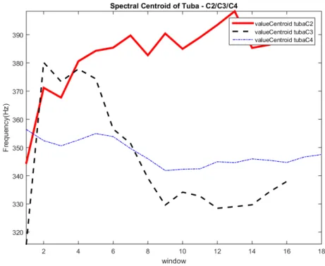
There is only one instrument that is an exception, which corresponds to the tuba. When analyzing the sounds of the tuba, we detected an unexpected variation of the spec-tral centroid and warmth. The variations of the specspec-tral centroid don’t follow what was mentioned earlier, since the tuba’s centroid is not varying proportionally to the pitch. We expected, between the three tuba sounds, that the values of the spectral centroid of tuba C2 were the lowest and the values of the spectral centroid of C4 would be the highest, however this does not happen as the values of the spectral centroid of tuba C2 are

(43)

high-3.2 Analysis of the instrumental sounds 19

Instruments Octave Weighted Arithmetic

Mean Variance Std Tuba C2 4.52 2.66 1.63 C3 4.4 2.32 1.52 C4 3.97 2.06 1.44 Horn C2 4.13 2.14 1.46 C3 3.2 1.74 1.32 C4 3.66 2.38 1.54 Clarinet C4 3.8 1.83 1.35 C5 2.95 1.75 1.32 C6 1.91 1.63 1.27 Oboe C4 2.82 1.32 1.15 C5 2.18 1.21 1.1 C6 1.77 1.49 1.22 Viola C3 3.83 1.78 1.34 C4 3.52 1.53 1.24 C5 2.95 1.86 1.37 Cello C3 4.58 1.96 1.4 C4 3.76 1.86 1.36 C5 2.96 1.9 1.38

Warmth Pearson correlation (rs)

0.022 p-value = 0.933457

Spectral Centroid Pearson correlation (rs)

-0.598 p-values = 0.009955

Table 3.3: Weighted arithmetic mean, variance and standard deviation of the results of the first listening test. The present Pearson correlation values result from a correlation between the values of warmth and the weighted mean values and also from a correlation between the values of the spectral centroid and the weighted mean values.

est. This can see see in FigureA.19. This might be due to a corruption in the audio files, which was only detect when performing a spectral analysis but didn’t affect the perceptual evaluation. For this reason, all sounds of the tuba won’t be, in the future, submitted to transformation by our system.

As we can observe from the values in Table3.3, the spectral centroid and the weighted mean of the evaluation present a high Pearson correlation of -0.59, albeit the warmth shows a not so satisfying Pearson correlation of 0.022. Furthermore, by looking at Figure 3.4we can verify that the spectral centroid correlates with the listeners responses because as said earlier, the spectral centroid varies proportionally with the weighted mean values. The sounds evaluated as warmer have a lower centroid, and the sounds evaluated as colder (less warm) have a higher centroid. Taking a look at Figure 3.5 we can’t correlate the warmth with the listeners’ evaluation.

In Figure3.6we have a linear regression between the sounds’ warmth and their spectral centroid. Most of the results are dispersed, leading us to the conclusion that there is no clear correlation between warmth and the spectral centroid. This conclusion is supported

(44)

Figure 3.2: Values of the spectral centroid of the violoncello C3 and oboe C6 sounds

(45)

Figure 3.4: Linear regression between the weighted arithmetic mean evaluation and the spectral centroid of all instrumental sounds

Figure 3.5: Linear regression between the weighted arithmetic mean evaluation and the warmth of all instrumental sounds

(46)

Instruments Octave Warmth Spectral Centroid Ratio between warmth and the spectral centroid

Tuba C2 0.29 382.23 0.075% C3 3.83 345.29 1.108% C4 66.95 347.95 19.241% Horn C2 0.22 484.42 0.045% C3 1.70 582.37 0.292% C4 4.54 619.72 0.733% Clarinet C4 1.34 1,095.70 0.122% C5 2.62 1,717.00 0.153% C6 23.00 1,981.50 1.161% Oboe C4 0.13 1,682.70 0.008% C5 1.79 2,034.00 0.088% C6 2.34 1,219.50 0.192% Viola C3 0.39 1,712.90 0.023% C4 0.37 1,757.70 0.021% C5 0.35 2,226.30 0.016% Cello C3 0.87 1,219.50 0.071% C4 0.31 1,684.00 0.019% C5 1.07 2,354.80 0.046% Pearson correlation (rs) -0.279 p-value = 0.262218

Table 3.4: Values of warmth and spectral centroid of each instrumental sound. A ratio between the warmth and the spectral centroid is also calculated. The present Pearson correlation value result of correlation between the values of warmth and the values of the spectral centroid

by the correlation value present in Table3.4where the the values of warmth and the values of the spectral centroid have a poor Pearson correlation of -0.279.

(47)

Figure 3.6: Linear regression between the warmth and the spectral centroid of all instru-mental sounds

(48)

(49)

Chapter 4

Development of the system

In this chapter we describe, in detail, the development of the system, created in Pure Data[35], that allows producers and musicians to manipulate the warmth of monophonic harmonic audio in real-time (e.g., of a live performance).

4.1 System Overview

Based on the new linear combination resulting from our listening test, we developed a (one-knob) audio effect which allows users to transform the warmth of a sound in real-time. To this end, we regulate the amplitudes of the spectral components of a musical audio, to shape them according to a relative user-controlled level of warmth. In other words, we allow user to dynamically reduce or increase the percentage of warmness in the musical audio input while retaining the relative variability over time.

Yet, due to its subjective nature, it’s hard to define it with a mathematical model, which would enable us to manipulate sounds using digital signal processing techniques. Therefore, by being aware of the importance of such a processing tool, we strive here to first understand the timbral attributes which impact such an informal sonic attribute and secondly encode it as a mathematical model which can be used to manipulate the warmth of musical audio in real-time.

The architecture of our system is shown in Figure4.1. After receiving the input audio file, the system first calculates the warmth region (WR) and the remainder magnitude (RM) as outputs. These outputs are then processed by a resynthesis algorithm. This algorithm takes the user input, which will control the level of warmth that he wants in the output audio file.

4.2 Definition of the Warmth Region

In order to define the warmth region, we use Williams and Brookes’ metric, explained in Section2.5.1.1. They defend that the warmth region is the area encompassing the energy

(50)

Figure 4.1: System Architecture

of the first three harmonics.

Following [1], we define the warmth region as a ratio between the energy of the first three harmonics (WR) - using Equation2.14- and the remainder magnitude (RM) of the spectrum - using Equation 2.15.

For this we developed a routine using Pure Data programming environment [35], that can be seen in Figure A.2. In the core of the patch is the use of Sigmund, a sinusoidal analysis and pitch tracking pure data object, developed by Puckette, that allows us to acquire information regarding the envelope, the peaks and pitch from the audio file. Since we are analyzing audio files, with a sampling rate of 441kHz, we use an analysis windows of 8192 samples which gives us an adequate frequency resolution for spectral analysis, as seen in Table 4.1using Equation4.1. The hop (number of points between analysis) is one fourth of the analysis windows (2048).

Number of bins of the FFT (N) 128 256 512 1024 2048 4096 8192 Lowest Detectable

Frequency (Hz) 344.53 172.27 86.13 43.07 21.53 10.77 5.38 Table 4.1: Lowest Detectable Frequency according to the FFT window size, considering 44100Hz the sampling rate

d f = fs

N (4.1)

Where:

df is the Lowest Detectable Frequency (frequency resolution); fs is the sampling rate;

N is the number of sample acquired.

After analyzing the spectrum in the warmth region, we create a table which contains the information of the first three harmonics. This table is then sent to the resynthesis

(51)

4.3 Resynthesis 27

module, which is explained in the following section (Section 4.3). Figure 4.2 shows the first three harmonics of thf viola C4 sound.

Figure 4.2: First three harmonics of a Viola C4 sound

4.3 Resynthesis

The resynthesis module is responsible for filtering the audio signal and then modify its amplitude based on a user input, in order to sound warmer or colder.

The algorithm starts by multiplying the audio with an Hann window, with half the size of the Fast Fourier Transform (FFT) window, in order to reduce the amplitude of the discontinuities at the boundaries of each block sequence. Then, it performs an FFT with a window size of 8192 Hz (Table4.1), with an overlap of four sequence blocks. In Figure 4.3 we see an example where the window size is n and the hop size is one fourth of the window size.

Figure 4.3: Example of a window with overlap of four blocks

Then, we perform a convolution of the audio and the received WR table. This table works as a band-pass filter and also as a reject-band filter.

(52)

As a band-pass filter (Figure4.4), it only allows the parts of the signal that are within the warmth region, in other word, between the central frequency and 3.5 times the central frequency, and all others frequencies are attenuated.

As a reject-band filter (Figure4.5) it does the opposite, allowing only the parts of the signal that are outside the warmth region.

Figure 4.4: Band-pass filter where only the values within the warmth region are allowed, and the rest is attenuated

Figure 4.5: Reject-band filter where the amplitudes within the warmth region are attenuated

At last, both signals are normalized and reconstructed to time domain using the In-verted Fast Fourier Transform (IFFT) and multiplied, once again, by the Hann window in order to correct the zero-crossing.Then, they go through a cross fade operation before outputting the audio file.

4.3.1 Crossfade

This module performs a crossfade between the signal corresponding to the warmth region and the signal corresponding to everything else, except the warmth region. This operation consists in the manipulation of the the warmth region according to a variation of a user input value.

cross f ade= A + X ˙B (4.2)

Where:

A corresponds to the signal after passing through the band-pass filter; B corresponds to the signal after passing through the reject-band filter; X corresponds to a value controlled by a user input.

(53)

Chapter 5

Evaluation of the system

This chapter starts by explaining the listening experiment used to evaluate the effectiveness of the system. Then we present and comment on the results from the listening test.

Lastly, we analyze the new values of warmth and spectral centroid of the transformed sounds and compare them to their original sound.

5.1 Listening Test

In order to evaluate the performance of our system, we conducted a second online listening experiment1 of a set of instrumental sounds.

Based on the responses of the first listening test, the violoncello was the instrument with a warmer evaluation overall. In this regard, we selected the highest octave (C5) in order to evaluate if the variation of its warmth would be perceived. This same octave was selected for all the others instruments, except for the horn where we used the octave C4, which is the highest octave available.

To perform an objective evaluation of the system, we modified each instrument ac-cording to different degrees of warmth. Specifically, we increased the warmth by 25% and 50% and decreased the warmth by 25% and 50%. The test can be found in AppendixA.4. In the survey, participants were asked to rate on a 5-point Likert scale (1-5) the dif-ference in warmth between the two available audio, where 1 corresponds to the modified sound being much warmer than the original sound, 3 corresponds to no prominent differ-ence between the two sounds, and 5 corresponds to evaluating the modified sound as much colder than the original sound.

Before rating, the participants were asked to find a quiet place and listen to the full extent of both audio examples using high quality headphones.

In order to submit their ratings and complete the listening test, the participants were obliged to rate all sound examples. To prevent responses bias introduced by order effects, the musical examples were presented in a random order at each experiment trial.

1_{The listening test is available at}_{http://npires91.polldaddy.com/s/listening-test-2}

Computer Sound Transformations Guided by Perceptually Motivated Features

Faculdade de Engenharia da Universidade do Porto