Robotic-assisted approaches for image-controlled ultrasound procedures

(1)

2019

UNIVERSIDADE DE LISBOA

FACULDADE DE CIÊNCIAS

DEPARTAMENTO DE FÍSICA

Robotic-Assisted Approaches for Image-Controlled

Ultrasound Procedures

Guilherme Alexandre da Costa Correia

Mestrado Integrado em Engenharia Biomédica e Biofísica

Perfil em Engenharia Clínica e Instrumentação Médica

Dissertação orientada por:

Professor Rui Pedro Duarte Cortesão

Professora Guiomar Gaspar de Andrade Evans

(2)

(3)

ii

ACKNOWLEDGEMENTS

I would like to start by thanking Prof. Rui Cortesão for giving me the opportunity to join his research group at the Institute of Systems and Robotics of the University of Coimbra, and by all his support and guidance throughout the year. I would also like to thank Prof. Guiomar Evans for the patience, the orientation and for all the scientific advice.

I would like to thank my parents and my brother, for the unconditional support and motivation. A special thanks goes also to all my aunts and uncles, cousins, grandmother and grandfathers for all the fun moments, all the hugs, and all the encouragement. Thank you all for being always there for me.

My friends are a second family for me. To all of them: Cláudia, Beatriz, Nuno, Maria, Rita, João and Raquel, my heartfelt thanks for all the companionship, patience and support over these last five years.

(4)

iii

ABSTRACT

Ultrasound (US) systems are very popular in the medical field for several reasons. Compared to other imaging techniques such as CT or MRI, the combination of low-priced and portable hardware with real-time image acquisition enables great flexibility regarding medical applications, from simple diagnostics tasks to high precision ones, including those with robotic assistance. Unlike other techniques, the image quality and procedure accuracy are highly dependent on user skills for spatial ultrasound probe positioning and orientation around a region of interest (ROI) for inspection. To make diagnostics less prone to error and guided procedures more precise, and consequently safer, the US approach can be coupled to a robotic system. The probe acts as a camera to the patient body and relevant imaging information can be used to control a robotic arm, enabling the creation of semi-autonomous, cooperative and possibly fully autonomous diagnostics and therapeutics.

In this project our aim is to develop a semi-autonomous tool for tracking defined structures of interest within US images, that outputs meaningful spatial information of a target structure (location of the centre of mass [CM], main orientation and elongation). Such tool must accomplish real-time requirements for future use in autonomous image-guided robotic systems. To this end, the concepts of moment-based visual servoing and active contours are fundamental. Active contours possess an underlying physical model allowing deformation according to image information, such as edges, image regions and specific image features. Additionally, the mathematical framework of vision-based control enables us to establish the types of necessary information for controlling a future autonomous system and how such information can be transformed to specify a desired task.

Once implemented in MATLAB the tracking and temporal performance of this approach is tested in built agar-agar phantoms embedded with water-filled balloons, for stability demonstration, probe motion robustness in translational and rotational movements, as well as promising capability in responding to target structure deformations. The developed framework is also inside the expected levels, being compatible with a 25 frames per second image acquisition setup. The framework also has a standalone tool capable of dealing with 50 fps. Thus, this work lays the foundation for US guided procedures compatible with real-time approaches in moving and deforming targets.

Keywords:

(5)

iv

RESUMO

A aquisição de imagens de ultrassons (US) é atualmente uma das modalidades de aquisição de imagem mais implementadas no meio médico por diversas razões. Quando comparada a outras modalidades como a tomografia computorizada (CT) e ressonância magnética (MRI), a combinação da sua portabilidade e baixo custo com a possibilidade de adquirir imagens em tempo real resulta numa enorme flexibilidade no que diz respeito às suas aplicações em medicina. Estas aplicações estendem-se desde o simples diagnóstico em ginecologia e obstetrícia, até tarefas que requerem alta precisão como cirurgia guiada por imagem ou mesmo em oncologia na área da braquiterapia. No entanto ao contrário das suas contrapartes devido à natureza do princípio físico da qual decorrem as imagens, a sua qualidade de imagem é altamente dependente da destreza do utilizador para colocar e orientar a sonda de US na região de interesse (ROI) correta, bem como, na sua capacidade de interpretar as imagens obtidas e localizar espacialmente as estruturas no corpo do paciente.

De modo para tornar os procedimentos de diagnóstico menos propensos a erros, bem como os procedimentos guiados por imagem mais precisos, o acoplamento desta modalidade de imagem com uma abordagem robótica com controlo baseado na imagem adquirida é cada vez mais comum. Isto permite criar sistemas de diagnóstico e terapia semiautónomos, completamente autónomos ou cooperativos com o seu utilizador. Esta é uma tarefa que requer conhecimento e recursos de múltiplas áreas de conhecimento, incluindo de visão por computador, processamento de imagem e teoria de controlo.

Em abordagens deste tipo a sonda de US vai agir como câmara para o interior do corpo do paciente e o processo de controlo vai basear-se em parâmetros tais como, as informações espaciais de uma certa estrutura-alvo presente na imagem adquirida. Estas informações que são extraídos através de vários estágios de processamento de imagem são utilizadas como realimentação no ciclo de controlo do sistema robótico em questão. A extração de informação espacial e controlo devem ser o mais autónomos e céleres possível, de modo a conseguir produzir-se um sistema com a capacidade de atuar em situações que requerem resposta em tempo real.

Assim, o objetivo deste projeto foi desenvolver, implementar e validar, em MATLAB, as bases de uma abordagem para o controlo semiautónomo baseado em imagens de um sistema robótico de US e que possibilite o rastreio de estruturas-alvo e a automação de procedimentos de diagnóstico gerais com esta modalidade de imagem. De modo a atingir este objetivo foi assim implementada nesta plataforma, um programa semiautónomo com a capacidade de rastrear contornos em imagens US e capaz de produzir informação relativamente à sua posição e orientação na imagem. Este programa foi desenhado para ser compatível com uma abordagem em tempo real utilizando um sistema de aquisição SONOSITE TITAN, cuja velocidade de aquisição de imagem é de 25 fps. Este programa depende de fortemente de conceitos integrados na área de visão por computador, como computação de momentos e contornos ativos, sendo este último o motor principal da ferramenta de rastreamento.

De um modo geral este programa pode ser descrito como uma implementação para rastreamento de contornos baseada em contornos ativos. Este tipo de contornos beneficia de um modelo físico subjacente que o permite ser atraído e convergir para determinadas características da imagem, como linhas, fronteiras, cantos ou regiões específicas, decorrente da minimização de um funcional de energia definido para a sua fronteira. De modo a simplificar e tornar mais célere a sua implementação este modelo dinâmico recorreu à parametrização dos contornos com funções harmónicas, pelo que as suas variáveis de sistema são descritoras de Fourier. Ao basear-se no princípio de menor energia o sistema pode ser encaixado na formulação da mecânica de Euler-Lagrange para sistemas físicos e a partir desta podem

(6)

v

extrair-se sistemas de equações diferenciais que descrevem a evolução de um contorno ao longo do tempo. Esta evolução dependente não só da energia interna do contorno em sim, devido às forças de tensão e coesão entre pontos, mas também de forças externas que o vão guiar na imagem. Estas forças externas são determinadas de acordo com a finalidade do contorno e são geralmente derivadas de informação presente na imagem, como intensidades, gradientes e derivadas de ordem superior. Por fim, este sistema é implementado utilizando um método explicito de Euler que nos permite obter uma discretização do sistema em questão e nos proporciona uma expressão iterativa para a evolução do sistema de um estado prévio para um estado futuro que tem em conta os efeitos externos da imagem.

Depois de ser implementado o desempenho do programa semiautomático de rastreamento foi validado. Esta validação concentrou-se em duas vertentes: na vertente da robustez do rastreio de contornos quando acoplado a uma sonda de US e na vertente da eficiência temporal do programa e da sua compatibilidade com sistemas de aquisição de imagem em tempo real. Antes de se proceder com a validação este sistema de aquisição foi primeiro calibrado espacialmente de forma simples, utilizando um fantoma de cabos em N contruído em acrílico capaz de produzir padrões reconhecíveis na imagem de ultrassons. Foram utilizados padrões verticais, horizontais e diagonais para calibrar a imagem, para os quais se consegue concluir que os dois primeiros produzem melhores valores para os espaçamentos reais entre pixéis da imagem de US.

Finalmente a robustez do programa foi testada utilizando fantomas de 5%(m/m) de agar-agar incrustados com estruturas hipoecogénicas, simuladas por balões de água, construídos especialmente para este propósito. Para este tipo de montagem o programa consegue demonstrar uma estabilidade e robustez satisfatórias para diversos movimentos de translação e rotação da sonda US dentro do plano da imagem e mostrando também resultados promissores de resposta ao alongamento de estruturas, decorrentes de movimentos da sonda de US fora do plano da imagem.

A validação da performance temporal do programa foi feita com este a funcionar a solo utilizando vídeos adquiridos na fase anterior para modelos de contornos ativos com diferentes níveis de detalhe. O tempo de computação do algoritmo em cada imagem do vídeo foi medido e a sua média foi calculada. Este valor encontra-se dentro dos níveis previstos, sendo facilmente compatível com a montagem da atual da sonda, cuja taxa de aquisição é 25 fps, atingindo a solo valores na gama entre 40 e 50 fps.

Apesar demonstrar uma performance temporal e robustez promissoras esta abordagem possui ainda alguns limites para os quais a ainda não possui solução. Estes limites incluem: o suporte para um sistema rastreamento de contornos múltiplos e em simultâneo para estruturas-alvo mais complexas; a deteção e resolução de eventos topológicos dos contornos, como a fusão, separação e auto-interseção de contornos; a adaptabilidade automática dos parâmetros do sistema de equações para diferentes níveis de ruido da imagem e finalmente a especificidade dos potenciais da imagem para a convergência da abordagem em regiões da imagem que codifiquem tipo de tecidos específicos.

Mesmo podendo beneficiar de algumas melhorias este projeto conseguiu atingir o objetivo a que se propôs, proporcionando uma implementação eficiente e robusta para um programa de rastreamento de contornos, permitindo lançar as bases nas quais vai ser futuramente possível trabalhar para finalmente atingir um sistema autónomo de diagnóstico em US. Além disso também demonstrou a utilidade de uma abordagem de contornos ativos para a construção de algoritmos de rastreamento robustos aos movimentos de estruturas-alvo no a imagem e com compatibilidade para abordagens em tempo-real.

Palavras-Chave:

Ultrassonografia, procedimentos guiados por imagem, controlo visual, contornos ativos, momentos da imagem

(7)

vi

LIST OF FIGURES

Figure 1-1: Representation of the master-slave relationship between medical and robot workstations.

... 2

Figure 1-2: Depiction of the robot architecture of the TER system: (a) - CAD model of the 4DOF actuator frame; (b) - relaxed state of aMcKibben pneumatic muscle; (c) - Contracted state of a McKibben pneumatic muscle. [1] ... 3

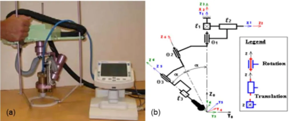
Figure 1-3: Depiction of the robot architecture of the OTELO system: (a) - Prototype of the light-weight 6DOF robot frame; (b) - Kinematic description of the robot frame motion in each DOF. [3] ... 3

Figure 1-4: Early developments of the ROSE robotic system implemented for a routine ovarian ultrasound diagnostic procedure. ... 4

Figure 1-5: Implementation of visual servoing techniques based on both image moments (a) and image quality (b) for US probe guidance and image optimization in a humanoid phantom. [13] ... 5

Figure 2-1: Representation of different image potentials: (a) - Line potential; (b) - Edge potential; (c) - Termination potential. ... 13

Figure 3-1: Scheme representing the experimental setup coupled with the tracking algorithm ... 25

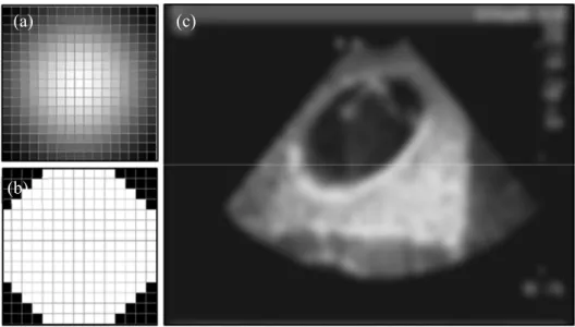
Figure 3-2: Image processing kernels: Gaussian kernel (a) and Circular kernel (b), along with their result on a sample image (c). ... 26

Figure 3-3: Scheme representing the overall organization of the tracking program. ... 27

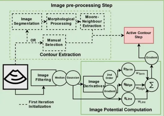
Figure 3-4: Scheme representing the organization of the image pre-processing step. ... 28

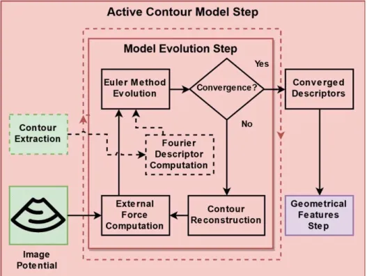
Figure 3-5: Scheme representing the organization of the active contour model step. ... 29

Figure 3-6: Scheme representing the organization of the geometrical features step. ... 30

Figure 4-1: Representation of the N-Wire phantom used in calibration: (a) - CAD model; (b) - the phantom weaved in a cross shaped pattern; (c) - the experimental setup for the calibration procedure. ... 32

Figure 4-2: Patterns implemented on the N-Wire phantom for calibration: (a) - Horizontal; (b)-Vertical; (c)- Diagonal... 33

Figure 4-3: Acquired images for a vertical (a), horizontal (b) and a diagonal pattern (c) on the calibration phantom. ... 33

Figure 4-4: The experimental setup used in the program performance testing routine. ... 36

Figure 4-5: Unwanted behaviour for contour evolution: (a) – Over sensitivity to image potentials; (b) – Convergence to a false image potential minimum; (c) – Unstable contour evolution. ... 37

Figure 4-6: Representation of the initial position in the performance testing routine , as shown in a CAD model (a) and in the real experimental setup (b)... 37

Figure 4-7: Representation of the in-plane motions induced in the performance routine, the vertical translation (a), the horizontal translation (b) and the in-plane tilting (c). ... 38

Figure 4-8:Representation of the out-of-plane motions induced in the performance routine, rotation on the probe axis resulting in contour deformation (a), out-of-plane translation resulting in contour contraction (b). ... 38

Figure 4-9: Visual representation of the tracking algorithm's GUI. ... 39

Figure 4-10: Acquired images for the tracking algorithm demonstrating translations in the horizontal direction (a)-(c), translations in the vertical direction(d)-(f) and in-plane tilting (g)-(i) for contour models with 3,6 and 9 harmonics. ... 39

Figure 4-11: Acquired images for the tracking algorithm demonstrating deformation via out-of-plane rotation (a)-(c) and contraction via out-of-plane translation (d)-(f) for contour models with 3,6 and 9 harmonics. ... 40

(10)

ix

LIST OF TABLES

Table 5-1: Results for the image calibration routine in mm/px. ... 34 Table 5-2: Set of parameters that define the desired behaviour for the contour model. ... 36 Table 5-3: Set of parameters for the base active contour model. ... 36 Table 5-4: Results of the measurement of the computation time of the tracking algorithms in ms. 40 Table 5-5: Results of the temporal performance testing of the algorithm as the mean frame rate. .. 40

(11)

x

LIST OF ABBREVIATIONS

CM – Centre of Mass

CT – Computed Tomography DOF – Degrees of Freedom fps – frames per second

MRI – Magnetic Resonance Imaging ROI – Region of Interest

(12)

1

CHAPTER 1 - INTRODUCTION TO ROBOTIC-ASSISTED

MEDICAL ULTRASOUND PROCEDURES

Due to the high-quality and often critical requirements of US tasks, the introduction of robotic systems in medicine is a growing practice in the development of medical applications, either in diagnostics or therapeutics. Since in many cases medical procedures require high precision and accuracy, it seems logical to introduce robotic systems for US tasks in order to be able to deliver expert-grade medical care to all citizens. Contrary to common belief, the main objective of robotic systems in medicine is not to replace the physician, but to provide better tools and information to enhance medical procedures, improving accurate diagnosis and promoting medical safety. Most of these systems work with a close relationship with the physician, where shared control strategies compensate for any unexpected and external disturbances. Additionally, in Globe regions where the availability of medical experts is reduced, such as in under-developed countries, the difference between life and death can many times be the introduction of robotic systems, that are autonomous, tele-operated or even cooperative, allowing remote experts to accurately treat or diagnose a patient at a distance and in real-time. One of the approaches that allows the creation such systems is the coupling of robotic technologies with image acquisition devices, allowing physicians to look and inspect inside the patient, for treatment or diagnosis. Due to mobility constraints and flexibility, ultrasound (US) imaging ends up being the most used technique where the acquired image integrates control of a medical procedures mediated by a robotic platform. With the objective of creating a future robotic system capable of delivering semi-automated medical diagnosis through ultrasound imaging, this M.Sc. thesis aims to develop a semi-autonomous tool for tracking defined structures of interest in US images, outputting meaningful spatial information of target structures in real-time. For this purpose, this dissertation is focused on the definition, implementation and validation of the base framework for image-controlled procedures.

1.1 Thesis Organization

The thesis is organized as follows. This first chapter covers different approaches for the inclusion robots that are tele-manipulated and image-controlled in the medical field, presenting several solutions and exposing their desirable features in terms of diagnostics and therapeutics. The second chapter lays the theoretical foundations for the creation of image-controlled systems, beginning with how a robot can respond to image features and how it can conciliate visual control with physician cooperation, and furthering into the underlying physical model that makes this possible. The third chapter addresses the schematic description on how a tracking algorithm is designed and implemented for the MATLAB platform and the fourth chapter covers the experimental setup to validate algorithm tracking properties. Finally, the last chapter discusses usability, pointing out current shortcomings and how they can be compensated.

(13)

2

1.2 State-Of-The-Art on Robotic-Assisted Ultrasound Procedures

In the rest of this chapter a description of the robotic systems that are nowadays being implemented in the medical medium, spanning from tele-operation to image guidance.

1.2.1 Tele-Operated Robotic Systems

Tele-operated robotic systems have the purpose of enabling expert-grade medical care to be available over large distances through interfacing medical experts with a purposely built robotic system. Such systems usually rely on two mechanical units: an end-effector and an actuator, meaning a tool through which the expert issues commands to the system and a robot architecture that will carry out the instruction, where, typically the communication between components is based on master-slave relationships. The communication between components, as described in Figure 1-1, is normally done through wireless network mediums, as Wi-Fi, 3G, 4G, through which important information needs to be sent bilaterally. This information includes actuator commands from master to slave as well as video stream and force feedback information, from slave to master, in order to guarantee accuracy and precision in the execution of diagnostics tasks.

Figure 1-1: Representation of the master-slave relationship between medical and robot workstations.

In the actuator department, early solutions, involve reduced DOF robots such as TER1_{with 4 DOF,} that dates back to 2002, as described in [1], which employs a soft approach of a robotic system. This robot employs a set of cables coupled to two parallel systems of antagonistic pressure-controlled artificial muscles, as depicted in Figure 1-2(a) . The first system allows the translation of a coupled probe along the patient’s surface and the second controls the orientation of the probe, thus enabling a total 3D control of the probe in the task space. Each of these systems are connected by artificial muscles, which are cylindrical rubber tube braided with a textile structure, with an air entry at an end and a plugged fixture at the other. Being a pneumatic system, when the pressure is raised each muscle contracts through conversion of the axial pressure forces into contraction forces by the textile shell, shortening the muscle length, as shown in Figure 1-2(b)-(c). Also, the muscle can act as a spring, whose stiffness is controlled through the pressure inside its cylinder, given the muscles are in an equilibrium position. This double compliance property allied with closed-loop position control, allow the system to adapt its contact force with the patients’ body for a force feedback approach.

(14)

3

Figure 1-2: Depiction of the robot architecture of the TER system: (a) - CAD model of the 4DOF actuator frame; (b) - relaxed state of aMcKibben pneumatic muscle; (c) - Contracted state of a McKibben pneumatic muscle. [1]

Another method is the OTELO2_{tele-echography system, described in [2], which has a different} approach, it uses a lightweight 6 DOF robot frame, enabling quick deployment of the system in isolated areas and for ER procedures in ambulatory voyages. The slave side consists of a mechanical structure coupled to a holding frame, shown in Figure 1-3(a), that is meant to be put on an area in the patient’s body, establishing a region of interest, that needs to be manually positioned by the acting physician on site. The system is underactuated, which means that not every degree of freedom is used for robot position control, in fact only five are used, three for orientation and two for translation in the directions perpendicular to the probes’ axis, as shown in Figure 1-3(b). The remaining degree of freedom, along the probe axis is designed to always maintain contact with the patient’s skin, allowing the expert to control the contact force between the probe and the skin, allowing force control feedback.

Figure 1-3: Depiction of the robot architecture of the OTELO system: (a) - Prototype of the light-weight 6DOF robot frame; (b) - Kinematic description of the robot frame motion in each DOF. [3]

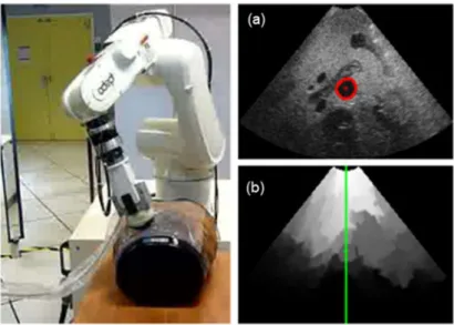
The construction and design of custom robotic frames can be costly and time consuming, both for design and licensing, as such other approaches rely on using readily available robot architectures well established in the industrial sector, such as in the ROSE project [4]. In the early settings of this system, an anthropomorphic 7-DOF WAM robotic arm has been used, as shown in Figure 1-4, with an integrated force sensor-driven adaptive control strategy adaptive compliant motion control based on online stiffness estimation. The system can respond either for compliant environments as in abdominal US or in rigid environments as in thoracic US. The system is also able to behave while in free space motion and switch to admittance control when it detects the probe is in contact with a surface. The ROSE project is currently using two lightweight robots from Haption that were customized for tele-ultrasound diagnosis.

(15)

4

As various diagnostic tasks require different applied forces, involving body areas with different rigidities (e.g., thoracic and abdominal ultrasound), the robotic system must adapt to conditions in order to provide the operator with the sense of tele-presence. As such, different control architectures have been deployed, as the ones described in [5] and [6], where the robot arm is ready to work in different rigidity regions, acting more or less compliant accordingly. Other approaches include motion compensation for robotic-assisted open tele-surgery of the heart [7] to provide a better working environment to the surgeon and enabling interventions without having to stop the organ itself, being less invasive to patient’s condition.

Figure 1-4: Early developments of the ROSE robotic system implemented for a routine ovarian ultrasound diagnostic procedure.

The common denominator in these approaches is the concern with accuracy of the procedures, which is an issue to be tackled both in the effector and human side of the equation. In the human side, the accuracy of the procedure is largely affected with the ability for the system to give haptic feedback to the operator. For this purpose, most master stations are equipped with haptic devices such as PHANTOM Omni. These devices have a defined workspace and can issue actuation commands with a resolution of 0.023 mm of resolution in the x, y and z directions, however, they are themselves joint actuated. Sets of motors in the joints enables a 3D sense of force resolution which allows the physician to experience the force feedback from the patient’s skin, enable to transduce stiffness information with a resolution of 1.90 N/mm, so that the operator can sense the features of the area in analysis.

1.2.2 Image-Controlled Robotic Systems

Even when the conditions for tele-operating ultrasound systems are favourable there can be unexpected situations or system-bound limitations that can diminish the accuracy of the diagnostic. Communications failure and lag are one of the main reasons for accuracy loss, but robot movement limitation, due to effector workspace limits, and image quality loss over distance can also impact the performance of the procedure. These and other numerable limitations push to the conclusion that a simple master-slave relationship architecture although necessary, can benefit from shared control between commands issued by the medical expert and automatic behaviour based on the in-situ acquired image. The control strategies which revolve around image acquisition, processing and therefore behaviour planning on the robot are grouped in as Visual Servoing strategies. One of the most prominent groups dedicated to investigation and implementation of these kinds of strategies is Alexandre Krupa’s Lagadic Group from IRISA (Institut de Recherche en Informatique et Systèmes Aléatoires) of the University of Rennes, having developed approaches that range from ultrasound guided needle insertion [8]–[10] to 3D ultrasound guidance using image speckle noise correlation to estimate out-of-plane motions of the probe [11], [12].

(16)

5

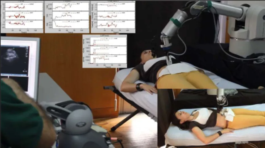
Figure 1-5: Implementation of visual servoing techniques based on both image moments (a) and image quality (b) for US probe guidance and image optimization in a humanoid phantom. [13]

Regarding visual servoing strategies it can be found that many approaches to the information present in an image can be taken to accomplish a panoply of behaviours: from tracking, to organ section search and probe adjustment. For instance, in [14] image moments of interest structures are used to prompt the robot to centre the probe in a specified organ section, as shown in Figure 1-5(a), allowing the robot to make both an automatic search in an area of interest for the pose of the probe that delivers the desired section and maintaining that pose over time. Other features, simpler or more complex, can be used to achieve the same behaviour, as described in [15], [16], where only through matching the pixel intensities between a desired and current image is enough to give reliable tracking results, while at the same time sparing time in image processing for systems with higher frame rates. Other applications use ultrasound image speckle and visual control for the automatic calibration of the robotized ultrasound probe system calibration [17], enabling the spatial reconstruction of a set of 2D US images along a line, in order to produce accurate probe localization in 3D space.

Lastly, another interesting application of visual servoing is described in [18]. In this case we have a tele-operated system that shares the control with an architecture that optimizes image quality. Using a model of propagation of ultrasounds along a scanning direction in tissue, an image quality map can be computed, defining which areas of the image are free from rigid tissue obstruction. The system can then compute which probe position maximizes the image quality in the central propagation line, shown in Figure 1-5(c), providing the medical expert with the best examination window possible with the least effort and time consumed.

Despite all the applications described earlier it can be pointed out that in a medical context the combination of the expertise of the acting physician with the accuracy of an automated system is yet to be completely achieved. This dissertation takes the path of visual servoing largely described by Krupa’s group and further develops this path for the purpose of semi-automatic diagnosis supported by ultrasound features and robotic technologies.

(17)

6

CHAPTER 2 - THEORETICAL FRAMEWORK

This chapter covers the theoretical aspects that comprise the implementation of a visual servoing based approach. The definition of a visual servoing framework is presented and the image processing tools necessary for tracking structures on US image are also defined.

2.1 Visual Servoing Framework

Visual servoing control is defined in [19] as a group of control strategies that use computer vision data to control the motion of a robotic system. This data can be acquired either from an imaging device (camera, US probe) coupled directly onto a robotic manipulator, in which the image motion is induced by the movement of the robot itself, eye-in-hand approach (EiH), or with a set of fixed imaging devices observing the workspace motion of the robot from a stationary position, eye-to-hand approach. These approaches rely on techniques from image processing, computer vision and control theory, and as such are based on the aim of minimizing an error, e(t), which is typically defined by:

𝑒(𝑡) = 𝑠(𝑚(𝑡), 𝑝) − 𝑠∗ _(3.1)

In general, the objective is to minimize the error vector, which can be defined as the difference of a measured feature vector 𝑠 and a desired feature vector 𝑠∗_{. In turn, the measured features vector can be} defined as a function of a set, 𝑚(𝑡), image feature measurements (i.e., coordinates of interest, object centroids, Etc.) and 𝑝, a set of parameters with additional information on the geometrical model of the acquisition system.

As a very general formulation, this expression encompasses an immense variety of approaches, as different sets of feature vectors can be defined for different applications or tasks. The size of the feature vector is also not fixed and is also dependent on the application. For instance, we have the many approaches taken by Krupa’s group. In [15], the proposed task is structure tracking and the feature vector is taken as the pixel intensity of an acquired image, which is compared to a reference image section to which the robot must navigate. In [20] the task is to position the robot on a desired section of a target organ, in such way that the only necessary information is given by the contour of the target itself, as such the feature vector is defined as a reduced set of information. As demonstrated the control schemes mainly differ in the definition of the feature vector, but once it is selected the design of the control law is simpler, being a velocity controller the most straightforward approach.

To establish a velocity controller, it is required to define a relationship between the temporal variations of the feature vector and the velocity of the moving imaging device. Defining the instantaneous velocity vector for the probe as 𝑉 𝑣 , 𝜔 , separating 𝑣 as the translational velocity and 𝜔 as the rational velocity, this relationship can be expressed as follows:

(18)

7

In which 𝐿 ∈ ℝ × _{is called the interaction matrix related to 𝑠, also called a feature Jacobian, that} can possibly consider both feature vector information and the acquisition system’s geometrical information. If we take (1) and (2) into account the variation of the feature error 𝑒(𝑡), can be expressed by a similar relationship:

𝑒̇ = 𝐿 𝑉 (3.3)

Usually the next step is to force an exponentially decreasing behaviour for the feature error, meaning that 𝑒̇ = −𝜆𝑒. If now we consider 𝑉 as a commanded velocity, we reach the basic control law for visual servoing:

𝑉 = −𝜆𝐿 𝑒 (3.4)

In which 𝐿 ∈ ℝ × _{is the Moore-Penrose pseudo-inverse matrix associated to the system´s} definition of interaction matrix. As in real-time approaches is nearly impossible to determine an exact value for the interaction matrix, an estimation operator must be defined. Usually the estimation taken is one as identifying the error interaction matrix with the feature interaction matrix, as such as that 𝐿 = 𝐿 , arriving at a final basic law:

𝑉 = −𝜆𝐿 (𝑠 − 𝑠∗₎ _(3.5)

Which dictates the probe velocities needed to apply to reach convergence to a desired feature vector. As the previous approach is a rough approximation it inserts uncertainty into the control law, revealing some initialization problems and non-exponential behaviour at start, which is why some authors prefer to define a more robust operator, such as:

𝐿 =1

2(𝐿 + 𝐿 ∗) (3.6)

Involving the interaction matrices computed both at a current feature vector position and on the desired position, which can guarantee a better overall behaviour and smooth trajectories both in the image space and in the robot’s task space.

As we aim to apply visual servoing to diagnostics scenarios, other control issues beyond image must be considered. Additionally, as the shape of target-structures in ultrasound imaging are highly dependent on the contact forces between the probe and the patient’s body, force control also needs to be addressed implicitly or explicitly, together with visual servoing. For instance, using switched control, in which one kind of control is turned on while the other one is turned off is always an option. More advanced approaches are however described in [21] enabling joint force and visual control and hierarchic control.

The principle of the first approach is to divide the various components of the commanded velocities in appropriate way. This means the definition of a partitioned control law and a partitioned interaction matrix, as in:

(19)

8

In this case we have separation of translational and rotational components. But in many cases even these components can be divided in order to better decouple the different degrees of freedom for 3D motion. If we have an underactuated system, it is possible to make an optimal approach in fusing two types of control using what is called the redundancy framework. The approach is based on the hierarchization of tasks, defining a primary and a secondary, where the constraints of the second are projected into the null space of the vision-based task. This means that the secondary task will not affect the regulation of the primary task error to zero. Defining the global error as:

𝑒 = 𝐿 𝑒 + 𝑃 𝑒 (3.8)

In which, 𝑒 is the newly defined global error and 𝑃 = 𝐼 − 𝐿 𝐿 , the null space projection matrix. This approach enables using unconstrained degrees of freedom to complete the secondary task, be it vision-based or force feedback related, for which in this case the set of features may be a constant set of contact forces.

2.2 Fourier Active Contour Model

Keeping close to the approach detailed in [22] after defining how the robot should be controlled, the focus must shift to image processing tools necessary to drive the implementation forward. We plan to follow a similar approach for tracking target structures in the framework of an active contours.

Defined first by Terzopoulos in [23], an active contour, also known as a snake, is an energy-minimizing curve that can be guided by external constraint forces and can be influenced by image bound forces to converge into specific image features, such as lines and edges. These contour models lock on to nearby features enabling their accurate localization and providing a unified solution to several computer vision problems, such as edge, line and subjective contour detection, motion tracking and even matching in stereo images. Unlike other detection techniques these models are active, which means they are always minimizing the functional that defines their global energy, which is the motor for their dynamic behaviour. Formally these models encompass a global energy defining functional to which two types of constraint forces contribute, internal and external forces. If we defined a curve parametrically by 𝐶(𝑢) = 𝑥(𝑢), 𝑦(𝑢) , then we can define the total snake energy as:

𝐸 = ∫ 𝐸 𝐶(𝑢) 𝑑𝑢 = ∫ 𝐸 𝐶(𝑢) + 𝐸 𝐶(𝑢) 𝑑𝑢 (3.9)

The internal energy term derives from the internal forces of the contour, associated with bending and the external derives from image constraint forces specifically defined to make the contour converge on the desired features.

Early implementations of active contours operated on non-parametrized contour, using greedy algorithms that compute forces applied on each point of the defined contour, which implies considering every point a variable, meaning an implementation time that grows with 𝒪 𝑁 , the number of ordered points that defines it, which for a detailed approach can become incompatible with real-time implementation.

(20)

9

2.2.1 General Parametric Formulation for Active Contours

One way to formulate this concept in a way that reduces the number of variables that are needed is to re-parametrize the contour. The general form for a curve parametrization is defined as follows:

𝐶 (𝑢) = 𝑥 + ∑ 𝑞 Φ (𝑢) (3.10)

In this expression 𝐶 is linearly defined and depends on parameter vector 𝑞 of dimension 𝑛, 𝑥 is a point belonging to the contour and Φ is a two-dimensional matrix belonging to a set of orthogonal or descriptor base functions. These descriptor functions can appear in many forms, such as in [24] where a polar function framework is used to drive an active contour approach, that although solving the algorithm runtime problem cannot support non-convex curves. In [25] the contour curve is defined in the B-Spline framework assuring smoothness constraints and, through reduced description with a parameter vector of curve nodes and weights, also reduces the run time making it compatible with real-time and robust to image noise.

Following the definition in [24], [26], [27] for the dynamic behaviour, we consider the system will converge to minimize its energy functional according to the Euler-Lagrange equation. Considering 𝑞, the vector of contour descriptors, as a vector of system variables, the kinetic energy, 𝑇, and the potential energy, 𝑈, of the contour must follow and are defined by the expressions:

− = 𝑄 (3.11)

𝑇 = ∫ 𝜇 ‖𝐶 ‖ 𝑑𝑢 (3.12)

𝑈 = ∫ (𝑘 ‖𝐶 ‖ + 𝑘 ‖𝐶 ‖ )𝑑𝑢 (3.13)

In this formulation Equation (3.11) is the embodiment of the energy minimization principle in the form of Euler-Lagrange equation, where:

𝑄 = ∫ 𝑓 (𝑢) ( )𝑑𝑢 (3.14)

and 𝑄 is the generalized external force applied to the contour relative to the variable component 𝑞 . Equation (3.12) is the definition of kinetic energy, in which:

𝐶 = = ∑ 𝑞̇ Φ (3.15)

and 𝜇 represents the linear mass density of the contour. Finally, Equation (3.13) is the definition of a contour’s potential energy according to Tikhonov’s regularization problem, where:

(21)

10

𝐶 = = ∑ 𝑞 Φ (3.17)

and 𝑘 represents the extension component and 𝑘 the curvature component of the potential energy term. Combining Equations (3.11) -(3.13) with (3.14) -(3.16), keeping in mind that ‖Φ‖ = Φ Φ, we arrive at:

= ∫ 𝜇 ∑ 𝑞̈ Φ Φ 𝑑𝑢

= ∫ 𝑘 ∑ 𝑞 Φ Φ + 𝑘 ∑ 𝑞 Φ Φ 𝑑𝑢 (3.18)

From the definition of generalized external force, we can divide 𝑓, the applied external force to each contour point, in two components: a viscous and the image bound (𝑓 = 𝑓 + 𝑓 ). Then we can define a viscous force distribution due to the medium in the form: 𝑓 = −𝛾𝐶 , as a regular viscous force would and the image bound forces as a conservative force, deriving from a potential, in the form: 𝑓 = −∇𝐸. As such we would reach the results:

∫ 𝑓 (𝑢) ( )𝑑𝑢= − ∫ 𝛾 ∑ 𝑞̇ Φ Φ 𝑑𝑢

Q (𝑞 ) = − ∫ 𝐸 (𝑢) ( )𝑑𝑢

(3.19)

Going back to Equation (3.11) and inputting all the previous results the system of differential equations that regulates the dynamic behaviour of a general parametric active contour:

𝑀𝑞̈ + 𝐶𝑞̇ + 𝐾𝑞 = 𝑄 (𝑞) (3.20)

The model vaguely represents a flat two-dimensional medium in which the contour floats, evolving though a force balance, where 𝑀 represents the inertia of the curve, 𝐶 represents the effect of the medium’s viscosity and 𝐾 represents the joined effect of the elasticity and bending forces of the contour, being normally decompose as 𝐾 = 𝐾 + 𝐾 . The definitions for these matrices derive from the previous model, and are defined as follows:

⎩ ⎪ ⎨ ⎪ ⎧ 𝑀 = [𝑀 ] = 𝜇 ∫ Φ Φ 𝑑𝑢 𝐶 = [𝐶 ] = 𝛾 ∫ Φ Φ 𝑑𝑢 𝐾 = 𝐾 = 𝑘 ∫ Φ Φ 𝑑𝑢 𝐾 = 𝐾 = 𝑘 ∫ Φ Φ 𝑑𝑢 (3.21)

(22)

11

2.2.2 Fourier Formulation for Active Contour

Following closely the approach introduced by Li, Krupa and Collewet in [26], [27], a contour can be re-parametrized by taking the Fourier series of its components. Starting from the following definition:

𝐶 (𝑢) = 𝑥(𝑢) 𝑦(𝑢) = 𝑎 𝑐 + 𝑎 𝑏 𝑐 𝑑 cos(𝑙𝑢) sin(𝑙𝑢) (3.22)

With 𝑢 ∈ [0,2𝜋] and 𝑎 , 𝑏 , 𝑐 , 𝑑 being the coefficients of the Fourier series decomposition. The information on the shape of a contour will be condensed in the form of coefficients representing the weights of different ellipses that are drawn in harmonic proportion. Developing (3.22) into the standard formulation, by expanding the Fourier series:

𝐶 (𝑢) = 𝑎_𝑐 + (𝑎 cos(𝑙𝑢) 0 + 𝑏 sin(𝑙𝑢) 0 + 𝑐 0 cos(𝑙𝑢) + 𝑑 0 sin(𝑙𝑢) ) (3.23)

A variable vector 𝑞 with size (4ℎ + 2 × 1) , can be defined as 𝑞 = (𝑎 , 𝑎 … 𝑎 , 𝑏 … 𝑏 , 𝑐 , 𝑐 … 𝑐 , 𝑑 … 𝑑 ), where ℎ represents the number of preserved harmonics, that encodes the contour shape information and from which a curve can be reconstructed. And the basis set of functions, Φ , becomes apparent in (3.23). As is recurrent from Fourier analysis the more harmonic coefficients preserved the more accurate the representation of a contour will be and for which Nyquist’s sampling theorem stands true. Meaning that for a contour of 𝑁 sample points the maximum number harmonics for accurate reconstruction of a contour from descriptors is 𝑁 2⁄ , after which aliasing effects corrupt the description.

This parametrization with elliptic Fourier descriptors holds the advantage over polar description in the sense that it is compatible with non-convex curves and that its description base is a fully orthogonal set of 2𝜋-periodic function, meaning that while determining the dynamics matrices only same index base functions will deal non-zero integral values, meaning these matrices can be defined only through their diagonal, shown as follows:

⎩ ⎪ ⎪ ⎪ ⎨ ⎪ ⎪ ⎪ ⎧ 𝑀 = 𝜇 diag (2𝜋, 𝜋 … 𝜋, 𝜋 … 𝜋,_{2𝜋, 𝜋 … 𝜋, 𝜋 … 𝜋)} 𝐶 = 𝛾 diag (2𝜋, 𝜋 … 𝜋, 𝜋 … 𝜋, 2𝜋, 𝜋 … 𝜋, 𝜋 … 𝜋) 𝐾 = 𝑘 diag (0, 𝜋𝑙 … 𝜋ℎ , 𝜋𝑙 … 𝜋ℎ , 0, 𝜋𝑙 … 𝜋ℎ , 𝜋𝑙 … 𝜋ℎ ) 𝐾 = 𝑘 diag (0, 𝜋𝑙 … 𝜋ℎ , 𝜋𝑙 … 𝜋ℎ , 0, 𝜋𝑙 … 𝜋ℎ , 𝜋𝑙 … 𝜋ℎ ) (3.24)

In order to simplify the system of equations, and according to [28], the mass of each contour point is defined as zero, meaning that 𝜇 = 0 and 𝑀 = [0], assuming a system where all inertial effects are neglected and/or undesired, the system of ODE’s is reduced to:

(23)

12

𝑞(𝑡)̇ = −C 𝐾𝑞(𝑡) + 𝐶 𝑄 (𝑞(𝑡)) (3.25)

For the system to be able to be implemented on a computer it needs to be discretized, which can be done identifying as 𝑞̇ = (𝑞 − 𝑞 )∆𝑡 and 𝑞 = 𝑞 , employing an explicit Euler’s method, we reach the iterative formula for the evolution of the contour in descriptor space:

𝑞 = (𝐼 − ∆𝑡𝐶 𝐾)𝑞 + ∆𝑡𝐶 𝑄(𝑞 ) (3.26)

This is a useful formulation because it resembles the definition of a discrete state-space defined system, like as follows:

𝑞[𝑛 + 1] = 𝐴 ∗ 𝑞[𝑛] + 𝐵 ∗ 𝑄 [𝑛]

𝑦[𝑛] = 𝐶 ∗ 𝑞[𝑛] (3.27)

Where 𝐴 = [𝐼 − ∆𝑡𝐶 𝐾] , 𝐵 = [∆𝑡𝐶 ] , 𝐶 = 𝐼 are the state matrices, 𝑞 is the state vector and 𝑄 acts as the input vector for the system.

2.2.3 Definition of External Image Forces

The premise of this model is its ability to converge into desired features that can appear in an US image for which it relies in the action of external forces specifically modelled to repel or attract the contour. As initially approached by Terzopoulos in [23], these forces may derive from definition of a global image energy functional, that can be defined by the linear combination of specific image functionals, as such:

𝐸 = 𝑤 𝐸 _(3.28)

In practice the specific energy functionals used here are the line, edge and termination functionals, as they are defined in [23].The simplest one, the line functional, can be expressed as the image intensity itself, then if we define it as 𝐼(𝑥, 𝑦), then the functional yields:

𝐸 = −𝐼(𝑥, 𝑦) (3.29)

Depending on the sign of its corresponding weight, 𝑤 , it will make the contour be attracted either to bright lines or dark ones.

The edge functional is defined based on the image gradient, meaning that changes in gradient is what defines an edge of the image. This term works well, in the sense that it can make the contour converge into an edge, however it has a limited range of operation, meaning that if the contour is defined very far away from it, it won’t converge in useful time. Other undesired result particular to the specific contour model implemented is that for very steep potentials, instead of converging, the contour simply oscillates about the desired edge, producing an erroneous result as well as consuming more time due to the algorithm never reaching a proper settling time. To compensate this behaviour, to smoothen and add capture range to the edge functional, before computing the gradients, the image is filtered with a gaussian smoothing kernel, 𝐺(𝜎), meaning the edge functional can be defined as:

(24)

13

𝐸 = −‖∇[G(σ) ∗ 𝐼(𝑥, 𝑦)]‖ (3.30)

The last functional used in this approach is the termination functional, it provides the contour with the ability to be attracted to line segment terminations, corners and sensitive to subjective contours. Using the previously defined smoothed image identifying 𝐶(𝑥, 𝑦) = G(σ) ∗ 𝐼(𝑥, 𝑦) , the functional is defined as the of the gradient angle 𝜃 in the perpendicular direction, introducing a measure of curvature:

𝐸 = 𝜕𝜃

𝜕𝑛 =

𝐶 𝐶 − 2𝐶 𝐶 𝐶 + 𝐶 𝐶

𝐶 + 𝐶 ⁄ (3.31)

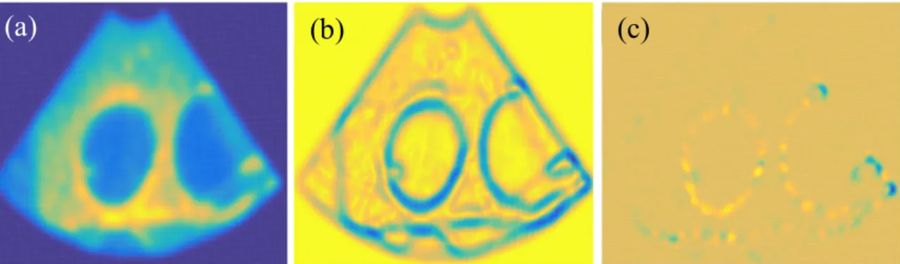
Where 𝐶 are the first and second order partial derivatives of the smoothed image. The combination of different functional weights can produce different but useful behaviours in the contour evolution. As an example, combining 𝐸 and 𝐸 , shown in Figure 2-1(b)-(c), with similar weights enables the contour to effectively converge into subjective edges. And combining 𝐸 , shown in Figure 2-1(a), and 𝐸 , enables an improved edge convergence depending on whether the region inside the contour is lighter or darker.

Figure 2-1: Representation of different image potentials: (a) - Line potential; (b) - Edge potential; (c) - Termination potential.

Due to the imaging principle of US, usually the image is corrupted with speckle noise, which is prejudicial to the convergence of active contours in the sense that it blurs edges and masks interest structures and the usual step is to preform speckle filtering, with bilateral or median filters. However, the image noise characteristics (mean and variance) can also be used in a statistical approach to an active contour algorithm. As described in [29], the external forces can be modelled recurring to the definition of a statistical image potential, derived from the measurement of the image mean, variance or even the introduction of a multivariate vector for region identification through convolution with texture kernels. This delivers an approach that can deal with image noise in a more robust way. Due to simplicity and time constraints our first iteration of implementing active contours will be based on image noise filtering.

2.3 Model Stability and Dimensioning

Along with the definition of the model for Fourier active contours, come a set of control parameters that ultimately define the dynamic behaviour of the model itself, which effects interact with one another to create the bigger picture. The set of parameters that directly affect the contour behaviour are 𝛾, 𝑘 and 𝑘 , due to altering the control matrices defined in (3.24), however, the parameter 𝑁 , the number of points in a contour and ℎ, the number of harmonics, also have effect, due to them changing the intrinsic

(25)

14

properties of the parametrization. Lastly, it is important to define the time step, ∆𝑡, for the algorithm, that defines how fast the contour algorithm will evolve.

2.3.1 Definition and Effects of Internal Force Parameters

Since the model is defined by a linear differential equation, thus translatable into a space-state system, these interactions between the effects of parameters are established by the eigenvectors of the state space matrix, which from (3.25) is identifiable as 𝐴 = −𝐶 (𝐾 + 𝐾 ). Since these are all diagonal matrices, their eigenvalues are their diagonal values, meaning, that each eigenvalue associated with each harmonic can be defined, as:

𝜆 = −𝑘 𝑙 + 𝑘 𝑙

𝛾 , 0 ≤ 𝑙 ≤ ℎ (3.32)

Since 𝑘 and 𝑘 are always positive the equation system is always stable since for every harmonic value the corresponding pole is on the left side of the complex plane. It is also useful to recognize that (3.32) is in fact a balance of forces between the internal forces of the contour and the viscous forces of the medium, since it can be used as a base definition tailor the behaviour of the system. For the parameters to be non-arbitrary we define another balance of forces, between the components of the internal force, elasticity and curvature. For a weak conditioning, these force balances can then be translated into the expressions:

0 ≤𝑘 ℎ + 𝑘 ℎ

𝛾 ≤ 𝛼, 𝛼 ∈ ℝ

0 ≤𝑘 ℎ

𝑘 ℎ ≤ 𝛽, 𝛽 ∈ ℝ

(3.33)

These balances are defined according to the harmonic of highest order, since they represent the eigenvalue with the highest value for fixed values of 𝛾, 𝑘 and 𝑘 . As such from the defined balances, with given choices of balance ratios, the conditions for the choice of parameters 𝑘 and 𝑘 become:

⎩ ⎪ ⎨ ⎪ ⎧ 0 < 𝑘 ≤ 𝛼𝛽𝛾 (𝛽 + 1)ℎ 𝑘 𝛽ℎ < 𝑘 ≤ 𝛼𝛾 − ℎ 𝑘 ℎ (3.34)

The definition of these ratios is also important to understand the physical behaviour of the system. As such, after analysing the ratio expressions and by experimental observation, for 𝛼 we can state that:

 If 0 < 𝛼 ≤ 1: We obtain contours mainly ruled by the viscous force from the medium, meaning that, it will sensitive to external forces, however producing a non-smooth evolution, since regularization terms are undervalued;

 If 𝑎 > 1: We obtain contours mainly ruled by internal forces, dealing low sensitivity to external forces but a smooth contour evolution.

(26)

15

For the case of ratio 𝛽, the balance for the components of internal force, we can state that:

 For 0 < 𝛽 ≤ 1: We obtain contours whose evolution is mainly conditioned by elastic forces. Meaning that the contour will contract rapidly, however since the curvature regularization term is undervalued, it might evolve forming sharp edges;

 For 𝛽 > 1: We obtain contours whose evolution is mainly conditioned by contour regularization forces. Meaning a slow contracting contour, whose curvature more rapidly evolves into unit at every point.

For a strong conditioning of the system, meaning a set of parameters with fixed ratios we have the expressions: ⎩ ⎨ ⎧𝑘 = 𝛼𝛽𝛾 (𝛽 + 1)ℎ 𝑘 = 𝛼𝛾 (𝛽 + 1)ℎ (3.35)

However useful a strong conditioning might look, it becomes limiting to the characteristics of the system, in the sense that one needs to know the exact value of the ratios for a given system configuration.

2.3.2 Viscous Force and Sensibility to External Forces

In order to define a measure of the contours’ sensibility to the action of external forces, the approach taken is like before, through force balances. As such, considering a system where the internal forces are null, we have 𝑞(𝑡)̇ _{= 𝐶} _{𝑄 (t), meaning the evolution is conditioned by the balance between viscous} force and the external force. In this case we can think of 𝑆 = ‖𝑑𝑞 𝑑𝑡⁄ ‖ = ‖𝐶 𝑄 ‖ as a global measurement for the action of external forces on the contour and as such if we can establish a global balance of forces as:

𝑆(𝑡) = ‖𝑄 (𝑡)‖

𝑠𝑞𝑟𝑡 𝜆 (𝐶) =

‖𝑄 (𝑡)‖

𝜋𝛾 (3.36)

To achieve a measure that is not time-dependent we have to define a mean sensitivity. This means defining an approach to define the mean 2-norm of the image acting force. For this we define a random force vector in which the applied force components (𝑥, 𝑦) to each point in the contour is a random variable with a standard Gaussian distribution [ 𝐹 ~ 𝑁(0,1) and 𝐹 ~ 𝑁(0,1) ]. Following transformation (11), the applied force is translated into the descriptor space, and since it defines a linear combination of the original force components with the components of 𝜕𝐶/𝜕𝑞, its own components are normally distributed [𝑄 ~𝑁(𝜇 , 𝜎 )] and since the mean for each cartesian component is zero we assume a priori that 𝜇 = 0. The next step is to take the 2-norm of the 𝑄 , this means the creation of yet another random variable, ‖𝑄 ‖ where:

‖𝑄 ‖ = 𝑄

(27)

16

To overcome the issue of having to estimate a mean vector and then its norm, the variance for each component is estimated and a general estimated variance is used to normalize the image force vector: 𝜎 = 𝑚𝑒𝑎𝑛(𝜎 , … 𝜎 ). As such we normalize and assume homoscedasticity such that:

‖𝑄 ‖

𝜎 =

1

𝜎 𝑄 ~ 𝜒 (𝑣) (3.38)

In this case 𝑣, should be 4ℎ + 2, however since we take assumptions, we can only aim to be significantly close. Through an iterative Monte-Carlo based process is possible to generate samples of random image forces, compute the estimators for the mean squared 2-norm and fit the chi-square distribution with 𝑣 degrees of freedom, allowing the definition of confidence intervals for that parameter. Since 𝐸 𝜒 (𝑣) = ‖𝑄 ‖ = 𝑣, then we can also estimate de confidence intervals for the values of the 2-norm of the force vector as:

‖𝑄 ‖ = 𝜎 𝑣 (3.39)

However, there must be acknowledgement that, since we make the assumption that all the means from the image force components are null, which is not always true, this estimation method for a high number of samples can overestimate the intervals for ‖𝑄 ‖. In order to compensate this effect, we must turn to the true distribution of ‖𝑄 ‖ , when 𝜇 ≠ 0, 𝑖 = 0, … ,4ℎ + 2, which is a non-central chi-square distribution:

‖𝑄 ‖

𝜎 =

1

𝜎 𝑄 ~ 𝜒 (𝑣 , 𝜆 ) (3.40)

Where the non-centrality parameter is 𝜆 = ∑ 𝜇 . This means that estimating the non-central distribution that fits the image force sample, yields:

‖𝑄 ‖ = 𝜎 (𝑣 + 𝜆 ) (3.41)

With this definition, the overestimation is somewhat compensated in the sense that the mean of the non-normalized 2-norm vector, falls within the confidence intervals for ‖𝑄 ‖ , that are derived from the intervals of the non-central distribution parameters. This estimation needs to be made each time we decide to use a different number of harmonics, since the higher the number of harmonics, the more sensible the contour. Finally, this yields our self-defined mean sensibility:

𝑆 =

𝜎 (𝑣 + 𝜆 )

(28)

17

2.3.3 Model Compensation with Balloon Force for Far Initialization

One of the main issues with the use of parametric active contours is their necessity to be initialized with a contour that lays in the neighbourhood of the desired features to be tracked. To deal with far contour initializations we could introduce pressure forces, as done in [25] that depend on the normal direction of the contour at each point, however that is time consuming so, as done in [24], yet another contour energy potential term is added to the internal forces, defined as 𝐸 = 𝑘 𝑆 . When 𝑘 > 0, we will have a fast-contracting contour, meaning better faraway initializations for features already inside the contour. When 𝑘 < 0, we can have expanding contours, enabling initialization of contours inside the features to be tracked. The force deriving from this potential proportional to the area enclosed by the contour is defined by means of the Green theorem as such as that:

𝑆 = ∫ 𝑥(𝑢) ( ) 𝑑𝑢 − 𝑦(𝑡) ( ) 𝑑𝑢

= 𝜋(∑ 𝑙(𝑎 𝑑 − 𝑏 𝑐 )) (3.43)

If we define the force as derivative of the potential for each harmonic, then 𝐾 = 𝜕𝐸 𝜕𝑞⁄ = 𝑘 𝑃𝑆𝑞, where:

𝑆 = diag (0, 𝜋𝑙 … 𝜋ℎ, 𝜋𝑙 … 𝜋ℎ, 0, 𝜋𝑙 … 𝜋ℎ, 𝜋𝑙 … 𝜋ℎ) And P is a permutation matrix defined as:

𝑃( ; ) = 𝑃( ; )= 0

𝑃( ; )= 𝑃( ; )= 1

𝑃( ; )= 𝑃( ; )= −1

𝑙 = 1, … , ℎ

(3.44)

This alternative representation of the 𝐾 matrix as linear operation mediated by a permutation matrix allows faster computation times because it avoids computing a permutation of vector 𝑞 at each iteration of the contour evolution and allows an analysis of the effect of this matrix in the general eigenvalues of the differential equation, meaning it can be used to better design the value of the scalar 𝑘 , that mediates this surface force. As such, with the balloon force effect the eigenvalues become:

𝜆 = −𝑘 𝑙 + 𝑘 𝑙 ∓ 𝑘 𝑙

𝛾 , 0 ≤ 𝑙 ≤ ℎ (3.45)

For previously fixed values of 𝑘 and 𝑘 , the positive eigenvalues introduced by this force do not affect the overall stability of the system, for 𝑘 > 0 and the same for negative eigenvalues, for 𝑘 < 0. However , this duality means that for 𝑘 > 0, 𝑘 𝑙 + 𝑘 𝑙 − 𝑘 𝑙 > 0 and that for 𝑘 < 0, 𝑘 𝑙 + 𝑘 𝑙 + 𝑘 𝑙 > 0, which allows to establish the global stability condition for each harmonic as:

𝑘

(29)

18

From this condition it can be established that if we desire a totally stable system, then the balloon force will always be significantly less important than the internal forces, which defeats the purpose of introducing this force as means of compensating the dynamics of the original system in order to make it converge faster, which however can be achieved by splitting condition (3.43) into two conditions. The rationale behind this separation is that the harmonic with the role of defining the global surface enclosed by the contour is the first one, ℎ = 1 , while the others deal with local areas related to contour deformation, for ℎ > 2. As such to control inflation or deflation of the contour, mediated by balloon force, we have: 𝑘 𝑘 + 𝑘 = 𝜌 𝑘 2𝑘 + 8𝑘 < 1 (3.47)

While the first condition establishes the force balance between internal forces and balloon force in the first harmonic of the contour the second guarantees that for higher harmonics the dynamic behaviour of the system remains stable. These conditions yield the definition of 𝑘 and bounds for 𝜌 as:

|𝑘 | = 𝜌(𝑘 + 𝑘 ) 0 < 𝜌 <2𝑘 + 8𝑘

𝑘 + 𝑘

(3.48)

In terms of contour the effects of the value of 𝜌 are as follows:

 For 𝑘 > 0: The contour always behaves in a contracting fashion regardless of the value of 𝜌. For values of ρ between zero and one, the additional contraction force is relatively less intense than the internal regularization forces, meaning that the contour evolves rapidly into an ellipse. For values bigger than one the contraction forces are predominant and the contour contracts in a less regulated fashion, allowing the formation of edges in the contour;

 For 𝑘 < 0: The contour presents two distinct behaviours, dependant on the value of 𝜌. For values between zero and one, the regularization forces are predominant over the expansion forces, meaning the contour will still contract, however at a lower rate and in with very smooth contour features. For 𝜌 = 1, the rate of contraction equals the rate of expansion and as such the global area remains the same, however since higher order harmonics are still at play the contour will regularize regardless, tending to an ellipse. For values between one and its maximal bound, the contour will acquire an expanding behaviour, which will enable initialization from the inside of structures of interest. An important note is that, since higher order harmonics are stable the contour will expand in the way best suited to the local shape of an interest structure, showing good sensibility to external and viscous force action.

(30)

19

2.3.4 Discrete System and Stability in Evolution

Since the model of the Fourier active contour defined is continuous, in order to be useful and implemented it needs to be in its discretized from, which was already defined in expressions (3.26) and (3.27), arriving at the discrete space-state model for the evolution of the contour. The discretization implies adding a final parameter to the model, ∆𝑡, the time step between iterations. Among other effects, this parameter will definitively command the speed of evolution of a contour and their overall stability in all harmonics over time of evolutions, meaning that the proper time step will either maintain the contour characteristics designed previously, slightly deviate from them, or turn the contour completely unstable. In order to makes this selection, we take from (3.27) the state-space matrix of the system, which in this case has eigenvalues defined as:

𝜆 = 1 −∆𝑡(𝑘 𝑙 + 𝑘 𝑙 ∓ 𝑘 𝑙)

𝛾 , 0 ≤ 𝑙 ≤ ℎ (3.49)

Since were in the discrete domain, in order for the contour model to be stable, then the modulus of all its eigenvalues must be contained in the unitary complex circle. Since all eigenvalues are dependent on the harmonics in a crescent manner, we need only to constraint the highest one to be sure all others are stable as well, which leads to the stability condition:

1 −∆𝑡(𝑘 ℎ + 𝑘 ℎ + 𝑘 ℎ)

𝛾 < 1 (3.50)

Considering that all other parameters are already fixed then, the time step can be bounded by:

0 < ∆𝑡 < 2𝛾

𝑘 ℎ + 𝑘 ℎ + 𝑘 ℎ (3.51)

With this condition we can choose the proper time step, however it should be used cautiously, for it does not distinguish oscillating stability with regular exponential stability. Again, since we are on the discrete domain, any eigenvalue with modulus less than one is considered stable however if its value is negative, we will have oscillating behaviour, which is ill advised due to reduced convergence of the active contour in these states. Splitting condition (3.52) in half we will have harmonics with all correspondent eigenvalues positive, which means overall smooth and contour evolution and convergence.

0 < ∆𝑡 < 𝛾

𝑘 ℎ + 𝑘 ℎ + 𝑘 ℎ (3.52)

If it is in our interest to be able to better control the smoothness, stability and evolution speed of the contour we can use (3.52) to place the poles in a determined interval. Using a parameter 𝑝 with value between zero and one, representing the minimum location of the last pole of the system, then fitting (3.52) between 𝑝 and one, then:

(31)

20 (𝑝 − 1)𝛾 𝑘 ℎ + 𝑘 ℎ + 𝑘 ℎ< ∆𝑡 < 𝛾 𝑘 ℎ + 𝑘 ℎ + 𝑘 ℎ (3.53)

The relationship between contour evolution speed and its smoothness and stability is inverse. Meaning that to achieve higher speeds of evolution we must compromise smoothness and stability.

2.4 Re-dimensioning of the Model

From the previous sections to determine the behaviour of an active contours model we have to define the set of control parameters. If there is the need to have a model with a similar behaviour that is based on a different number of harmonics or number of contour points then we need to define the re-dimensioning relations that allow the control parameters to be change while keeping the force balances that define behaviour constant.

2.4.1 Re-dimensioning for Different Number of Contour Points

The system’s behaviour will change with the number of points in a contour derived from changes in the internal forces potential energy, which is undesirable, since it forces us to define a different set of parameters for each value. This can be tackled by taking a reparameterization of the contour.

If as in [29] we admit the contour to be computationally defined by 𝐶(𝑢), where 𝑢 the index of its position in an array of 𝑁 points with 𝑢 = 1,2, … 𝑁 + 1, then applying and affine transformation as such as we get a contour defined by 𝐶∗_{(𝜇) = 𝐶}∗_{(𝑚𝑢 + 𝑏) , defined by 𝑁}∗_{points we can conclude that:}

𝜕 𝜕𝜇= 1 𝑚 𝜕 𝜕𝑢 𝑑𝜇 = 𝑚𝑑𝑢 (3.54)

Where 𝑚 = 𝑁∗_{/𝑁 . Inserting (52) into the internal potential energy definition (14) and forcing the} balance to be the same in each case, we get that the relationship between reparametrized parameters (𝑘∗,𝑘∗_{) and a set of base parameters (𝑘 ,𝑘 ) has to be:}

𝑘∗_{= 𝑁}∗_⁄_𝑁 _𝑘

𝑘∗= 𝑁∗⁄𝑁 𝑘 (3.55)

This possibility to reparametrize the models for different numbers of points opens the possibility to choose when to add or remove points from the contour for tracking of bigger or smaller structures, in which having a reduced and increased points is an advantage for capturing detail and for model stability.

2.4.2 Re-dimensioning for Different Number of Harmonics

As different levels of detail in the contour of an interest structure prompt higher number of harmonics in order to be described accurately, the active contour model needs to be able to preserve relationships between parameters in order to be fully useful. This means we need to establish transformations between parameters of from a model using ℎ harmonics and another using ℎ∗_{, while preserving the ratios derived} from the balance between forces.