EUROPEAN ORGANIZATION FOR NUCLEAR RESEARCH (CERN)
CERN-EP/2016-050 2016/10/10
CMS-HIG-13-032
Search for two Higgs bosons in final states containing two
photons and two bottom quarks in proton-proton collisions
at 8 TeV
The CMS Collaboration
∗Abstract
A search is presented for the production of two Higgs bosons in final states containing two photons and two bottom quarks. Both resonant and nonresonant hypotheses are
investigated. The analyzed data correspond to an integrated luminosity of 19.7 fb−1of
proton-proton collisions at√s =8 TeV collected with the CMS detector. Good
agree-ment is observed between data and predictions of the standard model (SM). Upper limits are set at 95% confidence level on the production cross section of new parti-cles and compared to the prediction for the existence of a warped extra dimension. When the decay to two Higgs bosons is kinematically allowed, assuming a mass scale
ΛR =1 TeV for the model, the data exclude a radion scalar at masses below 980 GeV.
The first Kaluza–Klein excitation mode of the graviton in the RS1 Randall–Sundrum model is excluded for masses between 325 and 450 GeV. An upper limit of 0.71 pb is set on the nonresonant two-Higgs boson cross section in the SM-like hypothesis. Limits are also derived on nonresonant production assuming anomalous Higgs bo-son couplings.
Published in Physical Review D as doi:10.1103/PhysRevD.94.052012.
c
2016 CERN for the benefit of the CMS Collaboration. CC-BY-3.0 license ∗See Appendix A for the list of collaboration members
1
1
Introduction
The discovery of a boson with a mass of approximately 125 GeV, with properties close to those expected for the Higgs boson (H) of the standard model (SM) [1, 2], has stimulated interest in the exploration of the Higgs potential. The production of a pair of Higgs bosons (HH) is a rare process that is sensitive to the structure of this potential through the self-coupling mechanism of the Higgs boson. In the SM, the cross section for the production of two Higgs bosons in pp
collisions at 8 TeV is 10.0±1.4 fb for the gluon-gluon fusion process [3–5], which lies beyond
the reach of analyses based on the first run of the CERN LHC.
Many theories beyond the SM (BSM) suggest the existence of heavy particles that can couple to a pair of Higgs bosons. These particles could appear as a resonant contribution in the invariant mass of the HH system. If the new particles are too heavy to be observed through a direct search, they may be sensed in the HH production through their virtual contributions (as shown, e.g., in Refs. [6, 7]); also, the fundamental couplings of the model can be modified relative to their SM values (as shown, e.g., in Refs. [8, 9]); in both cases, a nonresonant enhancement of the HH production could be observed.
Models with a warped extra dimension (WED), as proposed by Randall and Sundrum [10], postulate the existence of one spatial extra dimension compactified between two fixed points, commonly called branes. The region between the branes is referred to as bulk, and controlled through an exponential metric. The gap between the two fundamental scales of nature, such as
the Planck scale (MPl), and the electroweak scale, is controlled by a warp factor (k) in the metric,
which corresponds to one of the fundamental parameters of the model. The brane where the density of the extra dimensional metric is localized is called “Planck brane”, while the other, where the Higgs field is localized, is called “TeV brane”. This class of models predicts the existence of new particles that can decay to Higgs boson pair, such as the spin-0 radion [11–13], and the spin-2 first Kaluza–Klein (KK) excitation of the graviton [14–16].
There are two possible ways of describing a KK graviton in WED that depend on the choice of localization for the SM matter fields. In the RS1 model, only gravity is allowed to propagate in the extra-dimensional bulk. In this model the couplings of the KK-graviton to matter fields
are controlled by k/MPl[10], with the reduced Planck mass MPldefined by MPl/√8π. For the
possibility of SM particles to propagate in the bulk (the so-called bulk-RS model), the coupling of the KK graviton to matter depends on the choice for the localization of the SM bulk fields. This paper uses the phenomenology of Ref. [17], where SM particles are allowed to propagate in the bulk, and follows the characteristics of the SM gauge group, with the right-handed top quark localized on the TeV brane (so called elementary top hypothesis).
The radion (R) is an additional element of WED models that is needed to stabilize the size of the extra dimension l. It is usual to express the benchmark points of the model in terms of
the dimensionless quantity k/MPl, and the mass scaleΛR =
√
6 exp[−kl]MPl, with the latter interpreted as the ultraviolet cutoff of the model [18]. The addition of a scalar-curvature term can induce a mixing between the scalar radion and the Higgs boson [18, 19]. This possibility is discussed, for example, in Ref. [20]. Precision electroweak studies suggest that this mixing is expected to be small [21]. In our interpretations of the constraints we neglect the possibility of Higgs–radion mixing.
On one hand, the choice of localization of the SM matter fields for the KK-graviton resonance impacts the kinematics of the signal and drastically modifies the production and decay prop-erties [22]. The physics of the radion, on the other hand, does not depend much on the choice of the model [18], which obviates the need to distinguish the RS1 and bulk-RS possibilities.
Models with an extended Higgs sector also predict one spin-0 resonance that, when sufficiently massive, decays to a pair of SM Higgs bosons, and would correspond to an additional Higgs boson. Examples of such models are the singlet extension [23], the two Higgs doublet mod-els [24] (in particular the minimal supersymmetric model [25, 26]), and the Georgi-Machacek model [27]. The majority of these models predict that heavy scalar production occurs predomi-nantly through the gluon-gluon fusion process. The Lorentz structure of the coupling between the scalar and the gluon is the same for a radion or a heavy Higgs boson. Therefore the models for the production of a radion or an additional Higgs boson are essentially the same, provided the interpretations are performed in a parameter space region where the spin-0 resonance is narrow. The results of this paper can therefore be easily applied to constrain this class of mod-els.
Phenomenological explorations of the two-Higgs-boson channel were studied prior to the ob-servation of the Higgs boson [28], and, since then, other studies have become available [29–35]. Most of these indicate that in BSM physics an enhancement of the HH production cross sec-tion is expected, together with modified signal kinematics for the HH final state. This paper describes a search for the production of pairs of Higgs bosons in the γγbb final state in proton-proton (pp) collisions at the LHC, using data corresponding to an integrated luminosity of
19.7 fb−1 collected by the CMS experiment at √s = 8 TeV. Both nonresonant and resonant
production are explored, with the search for a narrow resonance X conducted at masses mX
between 260 and 1100 GeV.
The fully-reconstructed γγbb final state discussed in this paper, combines the large SM
branch-ing fraction (B) of the H→bb decay with the comparatively low background and good mass
resolution of the H → γγchannel, yielding a totalB(HH → γγbb)of 0.26% [36]. The search
exploits the mass spectra of the diphoton (mγγ), dijet (mjj), and the four-body systems (mγγjj), as
well as the direction of Higgs bosons in the Collins–Soper frame [37], to provide discrimination between production of two Higgs bosons and SM background.
A search in the same final state was performed by the ATLAS collaboration [38].
Complemen-tary final states such as HH →bbbb, HH→ττbb, and HH to multileptons and multiphotons
were also explored by the ATLAS [39, 40] and CMS [41–44] collaborations.
This paper is organized as follows: Section 2 contains a brief description of the CMS detector. In Section 3 we describe the simulated signal and background event samples used in the analysis. Section 4 is dedicated to the discussion of event selection and Higgs boson reconstruction. The signal extraction procedure is discussed in Section 5. In Section 6 we present the systematic uncertainties impacting each analysis method. Section 7 contains the results of resonant and nonresonant searches, and Section 8 provides a summary.
2
The CMS detector
The CMS detector, its coordinate system, and main kinematic variables used in the analysis are described in detail in Ref. [45]. The detector is a multipurpose apparatus designed to study
physics processes at large transverse momentum pT in pp and heavy-ion collisions. The
cen-tral feature of the apparatus is a superconducting solenoid, of 6 m internal diameter, providing a magnetic field of 3.8 T. A silicon pixel and strip tracker covering the pseudorapidity range
|η| < 2.5, a crystal electromagnetic calorimeter (ECAL), and a brass and scintillator hadron calorimeter (HCAL) reside within the field volume. The ECAL is made of lead tungstate crys-tals, while the HCAL has layers of plates of brass and plastic scintillator. These calorimeters
3
An iron and quartz-fibre Cherenkov hadron calorimeter covers larger values of 3.0< |η| <5.0.
Muons are measured in the|η| <2.4 range, using detection planes based on three technologies:
drift tubes, cathode strip chambers, and resistive-plate chambers.
The first level of the CMS trigger system, composed of special hardware processors, uses in-formation from the calorimeters and muon detectors to select the most interesting events in a time interval of less than 4 µs. The high-level trigger (HLT) processor farm further decreases the event rate from around 100 kHz to less than 1 kHz, before data storage.
3
Simulated events
The MADGRAPHversion 5.1.4.5 [46] Monte Carlo (MC) program generates parton-level signal
events based on matrix element calculations at leading order (LO) in quantum
chromodynam-ics (QCD), using LO PYTHIA version 6.426 [47] for showering and hadronization of partons.
The models provide a description of production through gluon-gluon fusion of particles with
narrow width (width set to 1 MeV) that decay to two Higgs bosons, with mass mH =125 GeV,
in agreement with Ref. [48]. Events are generated either for spin-0 radion production, or spin-2 KK-graviton production predicted by the bulk-RS model.
The samples for nonresonant production are generated considering the cross section
depen-dence on three parameters: the Higgs boson trilinear coupling λ, parametrized as κλ ≡λ/λSM,
where λSM≡m2H/(2v2) =0.129, with v= 246 GeV being the vacuum expectation value of the
Higgs boson; the top Yukawa coupling yt, parametrized as κt ≡ yt/ySMt , where ySMt = mt/v is
the SM value of the top Yukawa coupling, and mtthe top quark mass; and the coefficient c2of
a possible coupling of two Higgs bosons to two top quarks. The first two parameters reflect changes relative to SM values, while the third corresponds purely to a BSM operator. In this
parametrisation the SM production corresponds to the point κλ = 1, κt = 1 and c2 = 0. The
parameters κλ and c2 cannot be directly constrained by alternative measurements at the LHC.
Therefore we vary these parameters in a wide range: −20 ≤ κλ ≤ 20 and−3 ≤ c2 ≤ 3. The
range 0.75 ≤ κt ≤ 1.25 is compatible with constraints from the single Higgs boson
measure-ments provided in Ref. [49].
The part of the Higgs potential∆Lrelevant to two-Higgs boson production and their
interac-tions with the top quark can be expressed as in Ref. [50]:
∆L =κλλ
SMv H3−mt
v (v+κtH+ c2
vHH) (tLtR+h.c.), (1)
where tLand tRare the top quark fields with left and right chiralities, respectively, and H is the
physical Higgs boson field.
Besides being used to predict SM single-Higgs boson production, the MC predictions for the background processes are used also in comparisons with data, to optimize the selection crite-ria, and for checking background-estimation methods based on control samples in data. The dominant background, originating from events with two prompt photons and two jets in the
final state, is generated at next-to-leading-order (NLO) in QCD usingSHERPAversion 1.4.2 [51].
Multijet production with or without a single-prompt photon represents a subdominant
back-ground, and is generated with the PYTHIA 6 package. Other minor backgrounds, including
Drell–Yan (pp → Z/γ∗ → e+e−), SM Higgs boson production with jets, as well as vector
bo-son and top quark production in association with photons, are generated using MADGRAPH
and PYTHIA 6, or the generatorPOWHEG version 1.0 [52–54] at NLO in QCD. The generated
4
Event reconstruction
The events are selected using two complementary HLT paths requiring two photons. The first trigger requires an identification based on the energy distribution of the electromagnetic shower and loose isolation requirements on photon candidates. The second trigger applies tighter constraints on the shower shape, but a looser kinematic selection. The trigger
thresh-olds on the pT range between 26 and 36 GeV, and between 18 and 22 GeV, respectively, for
photons with highest (leading) and next-to-highest (subleading) pT, with specific choices that
depend on the instantaneous LHC luminosity. The HLT paths are more than 99% efficient for the selection criteria used in this analysis [57].
4.1 The H
→
γγ candidatePhoton candidates are constructed from clusters of energy in the ECAL [58, 59]. They are subsequently calibrated [60] and identified through a cutoff-based approach (referred to as
“cut-based analysis” in Ref. [57]). The identification criteria include requirements on pT of the
electromagnetic shower, its longitudinal leakage into the HCAL, its isolation from jet activity in the event, as well as a veto on the presence of a track matching the ECAL cluster. These criteria provide efficient rejection of objects that arise from jets or electrons but are reconstructed as
photons. Both photons are required to be within the ECAL fiducial volume of |ηγ| < 2.5.
Small transition regions between the ECAL barrel and the ECAL endcaps are excluded in this analysis, because the reconstruction of a photon object in this region is not optimal.
The directions of the photons are reconstructed assuming that they arise from the primary
ver-tex of the hard interaction. However on average≈20 additional pp interactions (pileup) occur
in the same or neighboring pp bunch crossings as the main interaction. Many additional ver-texes are therefore usually reconstructed in an event using charged particle tracks. We assume
that the primary interaction vertex corresponds to the one that maximizes the sum in p2
T of the associated charged particle tracks. For the simulated signal, it is shown that this choice of vertex lies within 1 cm of the true hard-interaction vertex in 99% of the events. With this choice for energy reconstruction and vertex identification, the diphoton mass resolution remains close to 1 GeV independent of the signal hypothesis.
Diphoton candidates are preselected by requiring 100< mγγ <180 GeV. The two photons are
further required to satisfy the asymmetric selection criteria pγ1
T /mγγ > 1/3 and p γ2 T /mγγ > 1/4, where pγ1 T and p γ2
T are the transverse momenta of the leading and subleading photons.
The use of different pT thresholds scaled by the diphoton invariant mass, minimizes turn-on
effects that can distort the distribution at the low-mass end of the mγγ spectrum. If there is
more than one diphoton candidate selected through the above requirements, the pair with the
largest scalar sum in the pTof the two photons is chosen for analysis.
4.2 The H
→
bb candidateThe Higgs boson candidate decaying into two b quarks is reconstructed following a procedure similar to that used in CMS searches for SM Higgs bosons that decay to b quarks [61].
The particle-flow event algorithm reconstructs and identifies each individual particle (referred to as candidates) with an optimized combination of information from the various elements of
the CMS detector [62, 63]. Then, the anti-kTalgorithm [64] clusters particle-flow candidates into
jets using a distance parameter D = 0.5. Jets are required to be within the tracker acceptance
(|ηj| < 2.4), and separated from both photons through a condition on the angular distance
in η×φ space of ∆Rγj ≡
√
4.3 The two-Higgs-boson system 5
The jet energy is corrected for extra depositions from pileup interactions, using the jet-area
technique [65] implemented in the FASTJET package [66]. Jet energy corrections are applied
as a function of ηj and pjT [67, 68]. Identification criteria are applied to reject detector noise
misidentified as jets, and the procedure is verified using simulated signal.
The identification of jets likely to have originated from hadronization of b quarks exploits the combined secondary vertex (CSV) b quark tagger [69]. This algorithm combines the informa-tion from track impact parameters and secondary vertexes within a given jet into a continuous output discriminant. Jets with CSV tagger values above some fixed threshold are considered as b tagged. The working point chosen in this analysis corresponds to an efficiency, estimated
from simulated multijet events, of≈70% and a mistag rate for light quarks and gluons of 1–2%,
depending on jet pT. This efficiency and the mistag rate are measured in data samples enriched
in b jets (e.g., in tt events). Correction factors of≈0.95 are determined from data-to-simulation
comparisons and applied as weights to all simulated events.
Events are kept if at least two jets are selected and at least one of them is b tagged. To improve signal sensitivity, events are subsequently classified in two categories: events with exactly one b-tagged jet (medium purity) and events with more than one b-tagged jet (high purity). In the
former category, the H → bb decay is reconstructed by pairing the b-tagged jet with a non
b-tagged jet, while in the latter category a pair of b-tagged jets is used. In both cases, when multiple pairing possibilities exist for the Higgs boson candidate, the dijet system with largest
pT is retained for further study. For medium- and high-purity simulated signal events, this
procedure selects the correct jets in more than 80% and more than 95%, respectively.
The resolution in mjj improves from 20 GeV for mX = 300 GeV to 15 GeV for mX = 1 TeV in
the high-purity category, and from 25 GeV for mX = 300 GeV to 15 GeV for mX = 1 TeV in the
medium-purity category. In the search for a low-mass resonance, the dijet mass resolution is improved using a multivariate regression technique [61] that uses the global information from the events as well as the particular properties of each jet, in an attempt to identify the semi-leptonic decays of B mesons and correct for the energy carried away by undetected neutrinos. The relative improvement in resolution is typically 15%. For the high mass analysis and
non-resonant analysis the mjj resolution is better than for low mass analysis. The improvement
provided by the regression technique was found to be very limited. Therefore in those cases no regression was used.
Independent of whether a search involves the usage of jet energy regression, all jets are required to have pjT >25 GeV. Finally, we require that 60<mjj<180 GeV.
4.3 The two-Higgs-boson system
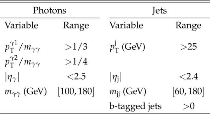
The object selections discussed thus far are summarized in Table 1.
In each category, two Higgs bosons are obtained by combining the diphoton and the dijet boson
candidates. To improve the resolution in mγγjj, an additional constraint is imposed requiring mjj
to be consistent with mH. This is achieved by modifying the jet 4-momenta using
multiplica-tive factors. The value of each factor is obtained event-by-event through a χ2 minimization
procedure where the size of the denominator is defined by the estimated resolution for each jet [70]. The procedure, similar to the one used in Ref. [70], is referred to as a kinematic fit and the resulting four-body mass is termed mkinγγjj.
The scattering angle, θHHCS, is defined in the Collins–Soper frame of the four-body system state,
Table 1: Summary of the analysis preselections.
Photons Jets
Variable Range Variable Range
pγ1 T /mγγ >1/3 p j T(GeV) >25 pTγ2/mγγ >1/4 |ηγ| <2.5 |ηj| <2.4 mγγ(GeV) [100, 180] mjj(GeV) [60, 180] b-tagged jets >0
line that bisects the acute angle between the colliding protons. In the Collins–Soper frame, the two Higgs boson candidates are collinear, and the choice of the one decaying to photons as
reference is therefore arbitrary. Using the absolute value of the cosine of this angle, cos θCS
HH , obviates this arbitrariness.
4.4 Backgrounds
The SM background in mγγcan be classified into two categories: the nonresonant background,
from multijet and electroweak processes, and a peaking background corresponding to events from single-Higgs bosons decaying to two photons.
After the baseline selections of Table 1, the dominant nonresonant background with two prompt
photons and more than two extra jets, referred to as γγ+ ≥2 jets, represents≈75% of the total
background. The nonresonant background with one prompt photon and a jet misidentified as
a photon as well as more than two extra jets, referred to as γ jet+ ≥ 2 jets, represents in turn
≈25%. The background from two jets misidentified as photons is negligible.
The remaining nonresonant and resonant backgrounds contribute much less than 1% to the total. They represent associated production of photons with top quarks or single electroweak bosons decaying to quarks, and Drell–Yan events with their decay electrons misidentified as photons. The resonant backgrounds correspond to different SM processes contributing to single-Higgs boson production.
All nonresonant backgrounds are estimated from data, and the resonant background from SM single-Higgs boson production in different channels is taken from the MC simulation normal-ized to NLO or next-to-NLO (NNLO) production cross sections, whichever are available [36].
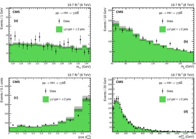
The comparison between data and MC predictions is provided in Fig. 1. The γγ/γ jet+ ≥2 jets
background is normalized to the total integral of data in the signal free region, defined by the condition mγγ >130 or mγγ <120 GeV in addition to the selections of Table 1.
5
Analysis methods
In the final step, this analysis exploits kinematic properties of the final state to discriminate
either resonant or nonresonant signal from SM background: the Higgs boson masses mγγ and
mjj, the cosine of their scattering angle cos θCS
HH
, and the mass of the two-Higgs-boson system,
mkin
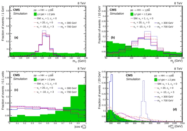
γγjj. Distributions in these variables are shown for different signal assumptions in Fig. 2. The
signal peaks in mγγ and mjj are shown in Figs. 2(a) and (b). The corresponding distributions
for the QCD background are smoothly varying over the shown ranges. The cos θCSHH
7 (GeV) γ γ m 116 118 120 122 124 126 128 130 132 134 Events / 1 GeV 10 20 30 40 50 60 (a) b b γ γ → HH → pp Data jets 2 ≥ jet + γ / γ γ (8 TeV) -1 19.7 fb CMS (GeV) jj m 60 80 100 120 140 160 180 Events / 10 GeV 50 100 150 200 250 (b) b b γ γ → HH → pp Data jets 2 ≥ jet + γ / γ γ (8 TeV) -1 19.7 fb CMS | CS HH θ |cos 0 0.1 0.2 0.3 0.4 0.5 0.6 0.7 0.8 0.9 1 Events / 0.1 units 100 200 300 400 500 (c) b b γ γ → HH → pp Data jets 2 ≥ jet + γ / γ γ (8 TeV) -1 19.7 fb CMS (GeV) kin jj γ γ m 300 400 500 600 700 800 900 1000 1100 1200 Events / 20 GeV 20 40 60 80 100 120 140 160 180 200 220 (d) b b γ γ → HH → pp Data jets 2 ≥ jet + γ / γ γ (8 TeV) -1 19.7 fb CMS
Figure 1: Reconstructed spectra for data compared to the γγ/γ jet+ ≥2 jets background after
the selections described in Table 1 (selections on photons and jets and a requirement of at least one b-tagged jet): (a) mγγ, (b) mjj, (c)
cos θCS
HH
, and (d) mkin
γγjj. The hatched area corresponds
to the bin-by-bin statistical uncertainties on the background prediction reflecting the limited size of the generated MC sample. The comparison is provided for illustrative purpose, in the backgrounds, except the one coming from single-Higgs production, are evaluated from a fit to the data without reference to the MC simulation.
uniform for signal, as shown in Fig. 2(c), while it peaks toward one for background. Finally, a
resonant signal appears as a narrow peak in mkinγγjjspectrum, while the nonresonant signal has
a broad contribution as shown in Fig. 2(d).
The dominant background from non-resonant production of prompt photons and jets exhibits a kinematic peak around mkinγγjj≈300 GeV followed by a slowly falling tail at high mkinγγjj. In the
resonant case, we consider two strategies, one for mX close to the kinematic peak, and one for
mX heavier than the kinematic peak. A third strategy is considered for the nonresonant case,
since the signal distribution as function of mkinγγjj is broad. In all cases a categorization is used based on the number of b-tagged jets. All the strategies are summarized in Table 2 and briefly described below:
1. Resonant search in the low-mass region (260 ≤ mX ≤ 400 GeV): the events are selected
in a narrow window around the mX hypothesis in the mkinγγjj spectrum, and the signal
is identified simultaneously in the mγγ and mjj spectra. This approach avoids a direct
search for a resonance in the mkin
γγjjspectrum near the top of the kinematic peak of the SM
background.
(GeV)
γ γ
m 116 118 120 122 124 126 128 130 132 134 136
Fraction of events / 1 GeV
0 0.1 0.2 0.3 0.4 0.5 0.6 8 TeV b b γ γ → HH → pp jets 2 ≥ jet + γ / γ γ = 0 2 c = 1, λ κ SM: = 0 2 c = 20, λ κ = 3 2 c = -10, λ κ = 300 GeV X m = 700 GeV X m CMS Simulation (a) (GeV) jj m 60 80 100 120 140 160 180
Fraction of events / 10 GeV
0 0.05 0.1 0.15 0.2 0.25 0.3 0.35 0.4 0.45 0.5 8 TeV b b γ γ → HH → pp jets 2 ≥ jet + γ / γ γ = 0 2 c = 1, λ κ SM: = 0 2 c = 20, λ κ = 3 2 c = -10, λ κ = 300 GeV X m = 700 GeV X m CMS Simulation (b) | CS HH θ |cos 0 0.1 0.2 0.3 0.4 0.5 0.6 0.7 0.8 0.9 1
Fraction of events / 0.1 units
0 0.05 0.1 0.15 0.2 0.25 0.3 0.35 0.4 8 TeV b b γ γ → HH → pp jets 2 ≥ jet + γ / γ γ = 0 2 c = 1, λ κ SM: = 0 2 c = 20, λ κ = 3 2 c = -10, λ κ = 300 GeV X m = 700 GeV X m CMS Simulation (c) (GeV) kin jj γ γ m 300 400 500 600 700 800 900 1000 1100 1200
Fraction of events / 20 GeV
0 0.05 0.1 0.15 0.2 0.25 0.3 0.35 0.4 0.45 8 TeV b b γ γ → HH → pp jets 2 ≥ jet + γ / γ γ = 0 2 c = 1, λ κ SM: = 0 2 c = 20, λ κ = 3 2 c = -10, λ κ = 300 GeV X m = 700 GeV X m CMS Simulation (d)
Figure 2: Simulated spectra for the spin-0 radion signal at mX = 300 and 700 GeV, and for
some values of the anomalous couplings, compared to SM Higgs boson production and QCD background, after the selections described in Table 1 (selections on photons and jets and a requirement of at least one b-tagged jet): (a) mγγ, (b) mjj, (c)
cos θCS HH , and (d) mkin γγjj. All spectra are normalized to unity.
in a window around mH in both the mγγ and mjjspectra, and the signal is identified in
the mkinγγjjspectrum.
3. Nonresonant search: a selection is applied in the cos θHHCS
variable to reduce the
back-ground. In addition to the categorization in the number of b-tagged jets, a categorization
is applied in mkinγγjj by defining a high-mass region and a low-mass region. The signal is
identified simultaneously in the mγγand mjjspectra.
Table 2: Summary of the search analysis methods.
Signal hypothesis Select # categories Fit
(1) mX≤400 GeV mkinγγjj 2 (b tags) mγγ, mjj
(2) mX≥400 GeV mγγ, mjj 2 (b tags) mkinγγjj
(3) Nonresonant cos θCS
HH
4 (b tags, mkin
γγjj) mγγ, mjj
The nonresonant background is described through different functions such as exponentials, power-law, or polynomials in the Bernstein basis [57]. When the search is performed simul-taneously in the diphoton and dijet mass spectra, these functions are used to construct a two-dimensional (2D) probability density (PD) for the background in each category, following an approach similar to Ref. [71]. Otherwise, a one-dimensional (1D) PD is used. In all cases, we
5.1 Low-mass resonant 9
choose the background PD to minimize the bias on signal. The bias is always found to be at least a factor of 7 smaller than the statistical uncertainty in the fit, and can be safely neglected [1]. In each invariant mass distribution used to identify the signal, the signal PD is modeled, fol-lowing the same approach as in Ref. [57], through the sum of a Gaussian function and a Crystal Ball (CB) function [72], using the parameters extracted from fits to MC simulations. The
reso-lution parameters in both functions are kept independent, σxGfor the Gaussian and σxCBfor the
CB function, but in the fits to each of the channels (x =γγ, jj, γγjj), we let the µ parameter for
both the Gaussian and the CB component float, which provides three independent µxvalues.
Finally, we consider the contribution from SM single-Higgs boson production in 2D searches.
The gluon-gluon and vector-boson fusion processes are modeled in mγγ by a sum over
Gaus-sian and CB functions, and through a constant term in mjj. The associated production of vector
bosons that subsequently decay to jets, and the SM single-Higgs bosons are modeled in the same way as the signal. The parameters of the distribution are extracted from a fit to the MC simulation.
The total PD used for signal extraction corresponds to a sum over separate PD contributions from the signal component, single-Higgs boson production, and nonresonant backgrounds.
We also verify that 2D PD functions can be considered as uncorrelated between mγγ and mjj
within the statistical uncertainties. To obtain this result we calculated the correlation in data. The uncertainty in the correlation was estimated by generating pseudo-experiments from a
model assuming no correlation between mγγ and mjjand calculating the root mean square of
the resulting distribution.
5.1 Low-mass resonant
In addition to the preselections summarized in Table 1, each mass hypothesis has a selection
applied on mkinγγjj in a narrow window around mX. The window sizes increase with mX to
ac-count for the increasing experimental resolution from ∆mX = ±10 GeV at mX = 260 GeV to
∆mX=+−3120 GeV at mX =400 GeV.
A possible signal can be extracted from data using a simultaneous fit to the mγγand mjjspectra.
The sensitivity to the signal in this search is increased through the b jet energy regression that
improves the resolution of the signal in mjj. The background-only PD is a first-order polynomial
in the Bernstein basis and a power law in the medium- and high-purity categories, respectively, as shown in Fig. 3, together with their 68% and 95% confidence level (CL) contours for the selection optimized for the search with mX=300 GeV, 290<mkinγγjj<310 GeV.
As a cross-check, two alternative signal extraction techniques are tested. In one, a selection is
performed in the mjj spectrum, and the signal extracted in the mγγ spectrum. In the other, a
selection is performed in the mjjspectrum and the mγγjjspectrum is exploited, using a
normal-ization extracted from sidebands in the mγγ spectrum. The two procedures give compatible
results within the statistical uncertainties.
5.2 High-mass resonant
In addition to the requirements in Table 1, selections are applied on mγγand mjj, as summarized
in Table 3.
A possible signal can be extracted from a fit to the mkinγγjj distribution for mass points between
320 ≤ mkinγγjj ≤ 1200 GeV. The background-only PD is a power law for each category, and is
(GeV) γ γ m 100 110 120 130 140 150 160 170 180 Events / 1 GeV 0 1 2 3 4 5 6 7 8 9 (8 TeV) -1 19.7 fb CMS = 300 GeV X , m b b γ γ → HH → X → pp High-purity
Data Background model
68% CL 95% CL (GeV) jj m 60 80 100 120 140 160 180 Events / 10 GeV 0 2 4 6 8 10 12 14 (8 TeV) -1 19.7 fb CMS = 300 GeV X , m b b γ γ → HH → X → pp High-purity
Data Background model
68% CL 95% CL (GeV) γ γ m 100 110 120 130 140 150 160 170 180 Events / 1 GeV 0 2 4 6 8 10 12 14 (8 TeV) -1 19.7 fb CMS = 300 GeV X , m b b γ γ → HH → X → pp Medium-purity
Data Background model
68% CL 95% CL (GeV) jj m 60 80 100 120 140 160 180 Events / 10 GeV 0 5 10 15 20 25 30 35 (8 TeV) -1 19.7 fb CMS = 300 GeV X , m b b γ γ → HH → X → pp Medium-purity
Data Background model
68% CL 95% CL
Figure 3: Low-mass resonant analysis: fits to the nonresonant background contribution in
high-purity category to the mγγ (top-left) and mjj spectra (top-right), and similarly for
medium-purity category in bottom-left and bottom-right, respectively. The fits to the background-only hypothesis are given by the blue curves, along with their 68% and 95% CL contours. The selections are designed to search for a mX =300 GeV hypothesis: 290<mkinγγjj<310 GeV.
kinematic turn-on, while still ensuring full containment of signal for the mX ≥ 400 GeV mass
hypotheses. Single-Higgs boson production is a negligible background in this phase space region, and is absorbed into the parametrization of the nonresonant background.
5.3 Nonresonant
We apply a selection on cos θHHCS
in the search for nonresonant two-Higgs boson production.
To increase the sensitivity to a large variety of BSM topologies (see examples shown in Fig. 2),
an additional categorization is applied in mkinγγjj. For the SM-like topology in gg→HH
produc-tion, the mkinγγjjspectrum peaks roughly at 400 GeV, while for|κλ| & 10 the peak shifts down to
the kinematic threshold of mkinγγjj≈250 GeV. Large absolute values of the c2(|c2| ≈3) parameter
5.4 Signal efficiency 11
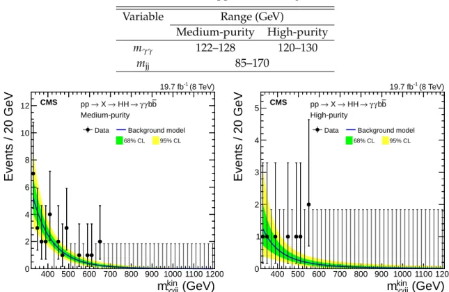
Table 3: Additional selection criteria applied in the high-mass resonant search.
Variable Range (GeV)
Medium-purity High-purity mγγ 122–128 120–130 mjj 85–170 (GeV) kin jj γ γ m 400 500 600 700 800 900 1000 1100 1200 Events / 20 GeV 0 2 4 6 8 10 12 (8 TeV) -1 19.7 fb CMS 68% CL 95% CL
Data Background model
b b γ γ → HH → X → pp Medium-purity (GeV) kin jj γ γ m 400 500 600 700 800 900 1000 1100 1200 Events / 20 GeV 0 1 2 3 4 5 (8 TeV) -1 19.7 fb CMS 68% CL 95% CL
Data Background model
b b γ γ → HH → X → pp High-purity
Figure 4: High-mass resonant analysis: fits to the nonresonant background contribution to the
mkinγγjjspectrum in medium- (left) and in high-purity (right) events. The fits to the
background-only hypothesis are given by the blue curves, along with their 68% and 95% CL contours.
categories are defined for mkin
γγjjsmaller or larger than 350 GeV, a value optimized for SM-like
search. The details of the selections and categorizations are provided in Table 4.
A possible signal can be extracted using a simultaneous fit to the mγγ and mjj spectra. The
background-only PD are exponentials and power-law expressions for the medium- and high-purity categories, respectively, which agree with the data, as can be seen in Figs. 5 and 6.
Table 4: Additional selections applied in the nonresonant searches.
Variable High-purity Medium-purity
cos θCSHH
<0.9 <0.65
mkinγγjjcategorization (GeV) <350 >350 <350 >350
5.4 Signal efficiency
The signal efficiency is a function of the mass hypothesis, as shown in Fig. 7. It is estimated with respect to all events generated in a given signal sample. The efficiency increases as the
resonance mass increases from mX = 260 to 900 GeV because of higher photon and jet
recon-struction efficiencies. The efficiency starts to drop for mX >900 GeV. At this point, the typical
angular distance in the laboratory frame between two b quarks produced in Higgs boson de-cay is of the order of the distance parameter D [73]. The minimum in efficiency is observed
at mX = 300 GeV. It results from an optimization procedure designed to maximize the
over-all analysis sensitivity. This procedure chooses an optimal size of mkinγγjj window for each mX
(GeV) γ γ m 100 110 120 130 140 150 160 170 180 Events / 1 GeV 0 1 2 3 4 5 6 7 8 9 (8 TeV) -1 19.7 fb CMS pp → HH →γγbb > 350 GeV kin jj γ γ High-purity, m
Data Background model
68% CL 95% CL (GeV) jj m 60 80 100 120 140 160 180 Events / 10 GeV 0 2 4 6 8 10 12 14 (8 TeV) -1 19.7 fb CMS pp → HH →γγbb > 350 GeV kin jj γ γ High-purity, m
Data Background model
68% CL 95% CL (GeV) γ γ m 100 110 120 130 140 150 160 170 180 Events / 1 GeV 0 2 4 6 8 10 12 14 (8 TeV) -1 19.7 fb CMS pp → HH →γγbb > 350 GeV kin jj γ γ Medium-purity, m
Data Background model
68% CL 95% CL (GeV) jj m 60 80 100 120 140 160 180 Events / 10 GeV 0 5 10 15 20 25 30 35 (8 TeV) -1 19.7 fb CMS pp → HH →γγbb > 350 GeV kin jj γ γ Medium-purity, m
Data Background model
68% CL 95% CL
Figure 5: Nonresonant analysis: fits to the nonresonant background contribution in high-mkinγγjj and high-purity category to the mγγ (top-left) and mjj spectra (top-right), and similarly
for medium-purity category in bottom-left and bottom-right, respectively. The fits to the background-only hypothesis are given by the blue curves, along with their 68% and 95% CL contours.
smallest, inducing a small drop in signal selection efficiency. Finally, the single and double b tag categories contribute in roughly equal ways to the total efficiency.
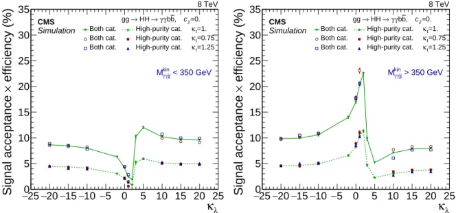
Figure 8 provides the efficiencies of selecting the signal events as function of κλ for different
values of κtand assuming c2 = 0. The left plot provides efficiencies for mkinγγjj < 350 GeV
cate-gories and right for mkinγγjj > 350 GeV categories. For large values of |κλ|(typically larger than
10) the efficiency is rather flat, while for small values of|κλ|the efficiency in the mkinγγjj<350 GeV
(mkinγγjj > 350 GeV) categories is reduced (increased). The change in efficiency is caused by the interference between two-Higgs box diagrams and the Higgs self coupling channel. The
to-tal efficiency in four categories is≈15–30%, depending on the model parameters. This figure
illustrates the way that mγγjjcategorization can help separate different nonresonant signal
5.4 Signal efficiency 13 (GeV) γ γ m 100 110 120 130 140 150 160 170 180 Events / 1 GeV 0 1 2 3 4 5 6 7 8 (8 TeV) -1 19.7 fb CMS pp → HH →γγbb < 350 GeV kin jj γ γ High-purity, m
Data Background model
68% CL 95% CL (GeV) jj m 60 80 100 120 140 160 180 Events / 10 GeV 0 2 4 6 8 10 12 14 (8 TeV) -1 19.7 fb CMS pp → HH →γγbb < 350 GeV kin jj γ γ High-purity, m
Data Background model
68% CL 95% CL (GeV) γ γ m 100 110 120 130 140 150 160 170 180 Events / 1 GeV 0 2 4 6 8 10 12 14 16 18 20 22 (8 TeV) -1 19.7 fb CMS pp → HH →γγbb < 350 GeV kin jj γ γ Medium-purity, m
Data Background model
68% CL 95% CL (GeV) jj m 60 80 100 120 140 160 180 Events / 10 GeV 0 10 20 30 40 50 (8 TeV) -1 19.7 fb CMS pp → HH →γγbb < 350 GeV kin jj γ γ Medium-purity, m
Data Background model
68% CL 95% CL
Figure 6: Nonresonant analysis: fits to the nonresonant background contribution in low-mkin
γγjj and high-purity category to the mγγ (top-left) and mjj spectra (top-right), and similarly
for medium-purity category in bottom-left and bottom-right, respectively. The fits to the background-only hypothesis are given by the blue curves, along with their 68% and 95% CL contours.
(GeV)
spin-0 Xm
300 400 500 600 700 800 900 1000 1100e
ff
ic
ie
n
c
y
(
%
)
×
Signal acceptance
0
10
20
30
40
50
60
b b γ γ → HH → X → ggAll cat. (Low-mass analysis) All cat. (High-mass analysis) High-purity cat. (Low-mass analysis) High-purity cat. (High-mass analysis)
8 TeV
CMS
Simulation
Figure 7: Resonant signal efficiency for the final selection described in Table 1 and Section 5. The efficiency is shown for a spin-0 hypothesis of a radion particle, but is similar for a spin-2 hypothesis of a KK graviton. The error bars associated with statistical uncertainties are smaller than the size of the markers.
λ κ 25 − −20−15−10−5 0 5 10 15 20 25 efficiency (%) × Signal acceptance 0 5 10 15 20 25 30 35 Both cat. Both cat. Both cat. =0. 2 c , b b γ γ → HH → gg =1. t κ High-purity cat. =0.75 t κ High-purity cat. =1.25 t κ High-purity cat. 8 TeV CMS Simulation < 350 GeV kin jj γ γ M λ κ 25 − −20−15−10 −5 0 5 10 15 20 25 efficiency (%) × Signal acceptance 0 5 10 15 20 25 30 35 Both cat. Both cat. Both cat. =0. 2 c , b b γ γ → HH → gg =1. t κ High-purity cat. =0.75 t κ High-purity cat. =1.25 t κ High-purity cat. 8 TeV CMS Simulation > 350 GeV kin jj γ γ M
Figure 8: Signal efficiency for c2=0 as function of κλfor different values of κt, for the low-mkinγγjj
region (left) and high-mkin
15
6
Systematic uncertainties
The analysis defines a likelihood function based on the total PD and the data. The parameters for total signal and for the background-only PD are constrained in the fit to maximize this func-tion. A uniform prior is used to parametrize the background PD. When converting the fitted yields into production cross sections, we use simulations to estimate the selection efficiency for the signal. The difference between the simulation and the data is corrected through scaling factors. The uncertainty in those factors is taken into account through parameters included in the likelihood function. The nuisance parameters (parameters not of immediate interest) are varied in the fit according to a log-normal probability density function. They can be classi-fied into three categories. The first category contains the uncertainty in the estimation of the integrated luminosity, which is taken as 2.6% [74]. The second category includes systematic uncertainties that modify the efficiency of signal selection. Finally the third category contains the uncertainties that impact the signal or the Higgs boson PD. More precisely, the values of the PD parameters are taken from fits to the MC simulation of signal and Higgs boson production. The systematic uncertainties affect the mean values and the resolution parameters of the PD, while all other CB parameters are fixed to their best values. The sources of nuisance parameters are described below and their contribution to different categories are presented in Table 5. The photon-related uncertainties are discussed in Ref. [57]. While the photon energy scale (PES)
is known at the sub-percent level in the region of pγTcharacteristic of the SM H→γγsignal, the
uncertainty increases to 1% for pγ
T > 100 GeV. The photon energy resolution (PER) is known
with a 5% precision [57]. A 1% normalization uncertainty is estimated in the offline diphoton selection efficiency and in the trigger efficiency. An additional normalization uncertainty of 5%
is estimated for the high-mass region to account for differences in the pT spectrum of signal
photons and of electrons from Z→ee production used to estimate the quoted uncertainties.
The uncertainty in the jet energy scale (JES) is accounted for by changing the jet response by 1–2% [68], depending on the kinematics, while the uncertainty in the jet energy resolution (JER) is estimated by changing the jet resolution by 10% [67]. An additional 1% uncertainty in the four-body mass accounts for effects in the high-mass region related to the partial overlap between the two b jets from the Higgs boson decay. The uncertainty in the b tagging efficiency is estimated by changing the b tagging scale factor up and down by one standard deviation in each purity category [69]. The related systematic uncertainties are known to be anticorrelated between the two categories.
Theoretical systematic uncertainties are considered for the single-Higgs boson contribution from SM production, corresponding to the scale dependence of higher-order terms and impact from the choice of proton parton distribution functions (PDF) [36, 75]. No theoretical uncertain-ties are assumed on BSM signals. However, there is one exception. We consider the situation where the kinematic properties of the new signal are identical to those of the SM, but the cross
section is different (SM-like search). In that case we parametrize the BSM cross section σBSM
HH by
the ratio µHH = σHHBSM/σHHSM. When such a search is performed the theoretical uncertainties on
σHHSMare included in the likelihood. Finally, an additional systematic uncertainty of 0.24 GeV is
assigned to account for the experimental uncertainty in the Higgs boson mass [48]. The impact of this uncertainty is comparable to the one from PES.
The analysis is limited by the statistical precision. The systematic uncertainties worsen the expected cross section limits by at most 1.5 and 3.8% in the resonant and nonresonant searches, respectively.
Table 5: Summaries of systematic uncertainties. For the normalization uncertainties, the values in the right column indicate the impact on the signal normalization. The uncertainty in the b
tagging efficiency is anticorrelated between the b tag categories. The uncertainty in the mkinγγjj
categorization is anticorrelated between mkin
γγjjcategories for the nonresonant search.
General uncertainties in normalization
Integrated luminosity 2.6%
Diphoton trigger efficiency 1.0%
Diphoton selection efficiency 1.0%
Resonant low-mass and nonresonant analyses: 2D fit to mγγand mjj
Uncertainties in normalization
—————-Acceptance in pjT( JES and JER) 1.0%
b tagging efficiency in the high-purity category 5.0%
b tagging efficiency in the medium-purity category
Low-mass resonant and nonresonant mkinγγjj<350 GeV 2.1%
Nonresonant mkinγγjj>350 GeV 2.8%
mkinγγjjacceptance (PES, JES, PER and JER)
Low-mass resonant 1.5%
Nonresonant mkinγγjj<350 GeV categories 1.5%
Nonresonant mkinγγjj>350 GeV categories 0.5%
Uncertainties in the PD parameters —————-mjjresolution (JER),∆σ G jj σGjj and ∆σCB jj σjjCB 10% mjjscale (JES), ∆µµjjjj 2.6% mγγresolution (PER), ∆σG γγ σγγG and ∆σγγCB σγγCB 5%
mγγscale (PES and uncertainty in mH)
Low-mass resonant, ∆µγγ
µγγ 0.4%
Nonresonant,∆µγγ
µγγ 0.5%
High-mass resonant analysis: 1D fit to mkinγγjj Uncertainties in normalization
—————-b tagging efficiency in the high-purity category 5.0%
b tagging efficiency in the medium-purity category 2.8%
mjjand pjTacceptance related to JES and JER 1.5%
mγγselection acceptance related to PES and PER 0.5%
Extra high pγT normalization uncertainty 5.0%
Uncertainties in the PD parameters —————-mkinγγjjscale (PES and JES), ∆µ
kin
γγjj
µkinγγjj 1.4%
mkinγγjjresolution (PER and JER), ∆σ
G, kin γγjj σG, kinγγjj and ∆σCB, kin γγjj σγγCB, kinjj 10.0%
17
7
Results
No significant excess is observed over the background expectation in the resonant or nonres-onant searches. Upper limits are computed using the modified frequentist approach for
con-fidence levels (CLs), taking the profile likelihood as a test statistic [76, 77] in the asymptotic
approximation. The limits are subsequently compared to theoretical predictions assuming SM branching fractions for Higgs boson decays.
7.1 Resonant signal
The observed and median expected upper limits for all the data at 95% CL are shown in the top of Fig. 9, and at the bottom in a zoomed-in view of the low-mass region. The expected limits
range from 1.99 fb for mX =310 GeV to 0.39 fb for mX =1 TeV. At the transition point between
the low-mass and high-mass searches, mX=400 GeV, results with both methods are provided.
An improvement of about 20% is observed from the use of the 2D model approach with respect to the 1D analysis.
The result is compared with the cross sections for KK-graviton and radion production in WED models. The tools used to calculate the cross sections for the production of KK graviton in the bulk and RS1 models are described in Refs. [78, 79]. The implementation of the calculations is described in Ref. [80]. In analogy with the Higgs boson, the radion field is predominantly produced through gluon-gluon fusion [81, 82]. The cross section for radion production is cal-culated at NLO electroweak and next-to-next-to-leading logarithmic QCD accuracy, using the recipe suggested in Ref. [18]. This recipe consists of multiplying the radion cross section based
on the fundamental parameter of the theory, ΛR, by a K-factor calculated for SM-like Higgs
boson production through gluon-gluon fusion [36, 83]. The calculations are performed for the SM-like Higgs boson with masses up to 1 TeV. We use the CTEQ6L PDF [84] in these calcula-tions. No mixing between a radion and the Higgs boson is considered in this paper.
In Table 6, we summarize the inclusive production cross sections and the branching fractions of the heavy resonances in the theoretical benchmarks we use for interpretation. The absolute
values of the production cross sections scale with(k/MPl)2for the KK Graviton [22] and with
1/Λ2
Rfor the radion [85].
The values for the branching fractions of the resonances in the theory benchmarks do not de-pend on the fundamental parameters of the theory. The resonance decays have a phase space suppression, related to the mass difference between the resonance and its decay products. In
this way, the decay to a Higgs boson pair is not allowed if mX<250 GeV nor to top quark pairs
if mX < 350 GeV. In Table 6, we see that the value of the branching fraction changes with the
resonance mass from mX = 300 to mX = 500 GeV. The exact pattern of this phenomenon is
related to the balance between the different phase space suppressions for decays to HH or to tt, which depends on the model under consideration.
The analysis excludes a radion with masses below 980 GeV for the radion scale ΛR = 1 TeV.
The search has also sensitivity to the presence of a radion with an ultraviolet cutoffΛR =3 TeV
in the region between 200 and 300 GeV.
The difference in total selection efficiency between the spin-0 (radion) and the spin-2 (KK-graviton) models does not exceed 3%. Thus, the same upper limits that are extracted using a radion simulation can be used directly to exclude a KK graviton with masses between 325
and 450 GeV, assuming k/MPl = 0.2. The analysis is not yet sensitive to the presence of a KK
Table 6: Cross section and branching fractions for the benchmark theories used in this paper [22,
85]. The branching fractions does not depend on k/MPl, nor onΛR.
Model mX(GeV) σ(gg→X)(pb) B(X→HH) RS1 KK graviton 300 2140 0.03% (k/MPl =0.2) 500 172 0.24% 1000 3.1 0.43% Bulk-RS KK graviton 300 0.65 0.89% (k/MPl =0.2) 500 0.11 8.2% 1000 0.0021 9.8% Radion 300 20.7 32% (ΛR =1 TeV) 500 3.87 25% 1000 0.46 24% (GeV) X m 300 400 500 600 700 800 900 1000 1100 ) (fb) b b γγ → HH → (X B × X) → (pp σ 2 − 10 1 − 10 1 10 2 10
= 0.2, elementary top, no r/H mixing Pl WED: kl = 35, k/M = 3 TeV) R Λ radion ( = 1 TeV) R Λ radion ( RS1 KK-graviton Bulk KK-graviton
Observed 95% upper limit Expected 95% upper limit
1 std. deviation ± Expected limit 2 std. deviation ± Expected limit (8 TeV) -1 19.7 fb CMS (GeV) X m 260 280 300 320 340 360 380 400 ) (fb) b b γγ → HH → (X B × X) → (pp σ 0 1 2 3 4 5 6 7 8
9 WED: kl = 35, k/MPl = 0.2, elementary top, no r/H mixing = 3 TeV)
R
Λ
radion (
RS1 KK-graviton
Observed 95% upper limit Expected 95% upper limit
1 std. deviation ± Expected limit 2 std. deviation ± Expected limit (8 TeV) -1 19.7 fb CMS
Figure 9: Observed and expected 95% CL upper limits on the product of cross section and the
branching fraction σ(pp → X) B(X → HH → γγbb)obtained through a combination of the
two event categories (left), and in the zoomed view at low-mass (right). The green and yellow bands represent, respectively, the 1 and 2 standard deviation extensions beyond the expected limit. Also shown are theoretical predictions corresponding to WED models for radions and RS1 KK gravitons. The upper plot with a logarithmic scale for the y-axis also provides the prediction for the production cross section of a bulk KK graviton. The vertical dashed line in the upper plot shows the separation between the low-mass and high-mass analyses. The limits
7.2 Nonresonant signal 19
7.2 Nonresonant signal
We consider the kinematic properties for new signal identical to those of the SM, but with a
different cross section. The observed and expected upper limits on SM-like gg→HH→γγbb
production are, respectively, 1.85 and 1.56 fb. This can be translated into 0.71 and 0.60 pb,
re-spectively, for the total gg→HH production cross section. The results can also be interpreted
in terms of observed and expected limits on the scaling factor µHH < 74 and<62+−3722, respec-tively. This result provides a quantification of the current analysis relative to the SM prediction. We also interpret the results in the context of Higgs boson anomalous couplings. The cross
section for nonresonant two-Higgs-boson production σHHBSM in this context can be written as a
polynomial in the parameters of the theory relative to the SM nonresonant cross section σHHSM
as: σHH σHHSM = A1κt4+A2c22+A3κt2κ2λ+ (A6c2+A7κtκλ)κ 2 t +A8κtκλc2. (2)
The numerical coefficients of Eq. (2) can be calculated by fitting cross sections as described in
Ref. [86], obtaining thereby: A1 = 2.19, A2 = 9.9, A3 = 0.324, A6 = −8.7, A7 = −1.51, and
A8 =3.0. Under the assumption that radiative corrections to gluon-gluon fusion of
two-Higgs-bosons do not depend significantly on anomalous interactions [87, 88], we normalize σHHsuch
that, when κt = 1, κλ = 1, and c2 = 0, to the cross section that equals the SM prediction at
NNLO in QCD.
In Fig. 10, 95% CL limits on nonresonant cross sections are shown, assuming changes only in
the trilinear Higgs boson couplings, with the other parameters fixed to their SM values. All κλ
values are excluded below−17.5 and above 22.5. These results are obtained by extrapolating
the limits between the simulated points, as well as above the highest simulated value of κλ
using Eq. 2, which relies on the similarity of distributions for signal at large values of|κλ|[86,
89], as well as on the behavior of the signal efficiency described in Section 5.4.
Figure 11 shows the 95% CL limits for nonresonant two-Higgs production in the c2 and κt
planes for different values of κλ. The specific interference pattern for each combination of
parameters produces different exclusion limits for different simulated points of parameter space [86, 89]. Only discrete values are provided for limits because a linear interpolation be-tween the simulated points could not follow the strong variations due to interference terms. The points in the theoretical phase space excluded by the data are surrounded by small black
boxes. Certain combinations of c2, κλ, or κt parameters can be excluded under the
assump-tion that Higgs bosons have their usual SM branching fracassump-tions. For example, we observe that
|c2| ≥3 is disfavored by the data when κλ and κtare fixed to SM values.
8
Summary
A search is performed by the CMS collaboration for resonant and nonresonant production of
two Higgs bosons in the decay channel HH → γγbb, based on an integrated luminosity of
19.7 fb−1of proton-proton collisions collected at√s = 8 TeV. The observations are compatible
with expectations from standard model processes. No excess is observed over background predictions.
Resonances are sought in the mass range between 260 and 1100 GeV. Upper limits at a 95% CL are extracted on cross sections for the production of new particles decaying to Higgs boson pairs. The limits are compared to BSM predictions, based on the assumption of the existence
of a warped extra dimension. A radion with an ultraviolet cutoff ΛR = 1 TeV is excluded
λ
κ
-20 -15 -10 -5 0 5 10 15 20 25
) (fb)
b
b
γγ
→
(HH
B
×
HH)
→
(pp
σ
10
-2 -110
1
10
(8 TeV)
-119.7 fb
CMS
Observed 95% upper limit Expected 95% upper limit
= 0., 2 c = 1.0, t κ Assuming SM H decays 1 std. deviation ± Expected limit 2 std. deviations ± Expected limit
Figure 10: Observed and expected 95% CL upper limits on the product of cross section and
the branching fraction σ(pp → HH) B(HH → γγbb)for the nonresonant BSM analysis,
per-formed by changing only κλ, while keeping all other parameters fixed at the SM predictions.
ultraviolet cutoffΛR=3 TeV when its mass lies between 200 and 300 GeV. The RS1 KK graviton
is excluded with masses between 325 and 450 GeV for k/MPl = 0.2. The analysis is not yet
sensitive to the presence of a KK graviton in the bulk scenario with the same parameters. For nonresonant production with SM-like kinematics, a 95% CL upper limit of 1.85 fb is set for the product of the HH cross section and branching fraction, corresponding to a factor 74 larger than the SM value. When only the trilinear Higgs boson coupling is changed, values of the self
coupling are excluded for κλ < −17 and κλ >22.5. The parameter space is also probed for the
presence of other anomalous Higgs boson couplings.
Acknowledgments
We are grateful to B. Hespel, F. Maltoni, E. Vryonidou, and M. Zaro for a customized model of the nonresonant signal generation.
We congratulate our colleagues in the CERN accelerator departments for the excellent perfor-mance of the LHC and thank the technical and administrative staffs at CERN and at other CMS institutes for their contributions to the success of the CMS effort. In addition, we grate-fully acknowledge the computing centres and personnel of the Worldwide LHC Computing Grid for delivering so effectively the computing infrastructure essential to our analyses. Fi-nally, we acknowledge the enduring support for the construction and operation of the LHC and the CMS detector provided by the following funding agencies: the Austrian Federal Min-istry of Science, Research and Economy and the Austrian Science Fund; the Belgian Fonds de la Recherche Scientifique, and Fonds voor Wetenschappelijk Onderzoek; the Brazilian Fund-ing Agencies (CNPq, CAPES, FAPERJ, and FAPESP); the Bulgarian Ministry of Education and Science; CERN; the Chinese Academy of Sciences, Ministry of Science and Technology, and
Na-21
(8 TeV)
-119.7 fb
CMS
1 - 1.5 fb 1.5 - 2 fb 2 - 2.5 fb 2.5 - 3 fb Excluded (Assuming SM H decays) Theoretical cross section AllowedObs. 95% CL upper limits ) b b γ γ → HH → (pp σ 3 − −2 −1 0 1 2 3 t
κ
0.4 0.6 0.8 1 1.2 1.4 κλ = 10 3 fb 2 fb 1 fb 0.2 fb 1 fb 3 − −2−1 0 1 2 3 0.4 0.6 0.8 1 1.2 1.4 κλ = -10 3 fb 2 fb 1 fb 0.2 fb 1 fb 0.4 0.6 0.8 1 1.2 1.4 κλ = 0 2 fb 1 fb 0.2 fb 0.2 fb 1 fb 2 fb = 15 λ κ 3 fb 2 fb 1 fb 0.2 fb 1 fb 3 − −2 −1 0 1 2 3 = -15 λ κ 3 fb 2 fb 1 fb 0.2 fb 1 fb tκ
0.4 0.6 0.8 1 1.2 1.4 = 1 λ κ 2 fb 1 fb 0.2 fb 0.2 fb 1 fb 2 fb 0.4 0.6 0.8 1 1.2 1.4 = 20 λ κ 3 fb 2 fb 1 fb 0.2 fb 1 fb 2c
3 − −2−1 0 1 2 3 0.4 0.6 0.8 1 1.2 1.4 = -20 λ κ 2 fb 1 fb 0.2 fb 1 fbFigure 11: The observed 95% CL limits for nonresonant two-Higgs production in the c2and κt
planes for different values of κλ. The different markers symbolize the range in which the upper
limits in the cross sections are relevant. The results are compared to the theoretical prediction. The gray lines represent contours of equal cross section, as calculated using Eq. (2). The boxed-in cross section markers provide the combboxed-ination of parameters excluded at 95% CL.
tional Natural Science Foundation of China; the Colombian Funding Agency (COLCIENCIAS); the Croatian Ministry of Science, Education and Sport, and the Croatian Science Foundation; the Research Promotion Foundation, Cyprus; the Ministry of Education and Research, Esto-nian Research Council via IUT23-4 and IUT23-6 and European Regional Development Fund, Estonia; the Academy of Finland, Finnish Ministry of Education and Culture, and Helsinki Institute of Physics; the Institut National de Physique Nucl´eaire et de Physique des Partic-ules / CNRS, and Commissariat `a l’ ´Energie Atomique et aux ´Energies Alternatives / CEA, France; the Bundesministerium f ¨ur Bildung und Forschung, Deutsche Forschungsgemeinschaft, and Helmholtz-Gemeinschaft Deutscher Forschungszentren, Germany; the General Secretariat for Research and Technology, Greece; the National Scientific Research Foundation, and Na-tional Innovation Office, Hungary; the Department of Atomic Energy and the Department of Science and Technology, India; the Institute for Studies in Theoretical Physics and
Mathe-matics, Iran; the Science Foundation, Ireland; the Istituto Nazionale di Fisica Nucleare, Italy; the Ministry of Science, ICT and Future Planning, and National Research Foundation (NRF), Republic of Korea; the Lithuanian Academy of Sciences; the Ministry of Education, and Uni-versity of Malaya (Malaysia); the Mexican Funding Agencies (CINVESTAV, CONACYT, SEP, and UASLP-FAI); the Ministry of Business, Innovation and Employment, New Zealand; the Pakistan Atomic Energy Commission; the Ministry of Science and Higher Education and the National Science Centre, Poland; the Fundac¸˜ao para a Ciˆencia e a Tecnologia, Portugal; JINR, Dubna; the Ministry of Education and Science of the Russian Federation, the Federal Agency of Atomic Energy of the Russian Federation, Russian Academy of Sciences, and the Russian Foun-dation for Basic Research; the Ministry of Education, Science and Technological Development of Serbia; the Secretar´ıa de Estado de Investigaci ´on, Desarrollo e Innovaci ´on and Programa Consolider-Ingenio 2010, Spain; the Swiss Funding Agencies (ETH Board, ETH Zurich, PSI, SNF, UniZH, Canton Zurich, and SER); the Ministry of Science and Technology, Taipei; the Thailand Center of Excellence in Physics, the Institute for the Promotion of Teaching Science and Technology of Thailand, Special Task Force for Activating Research and the National Sci-ence and Technology Development Agency of Thailand; the Scientific and Technical Research Council of Turkey, and Turkish Atomic Energy Authority; the National Academy of Sciences of Ukraine, and State Fund for Fundamental Researches, Ukraine; the Science and Technology Facilities Council, UK; the US Department of Energy, and the US National Science Foundation. Individuals have received support from the Marie-Curie programme and the European Re-search Council and EPLANET (European Union); the Leventis Foundation; the A. P. Sloan Foundation; the Alexander von Humboldt Foundation; the Belgian Federal Science Policy Of-fice; the Fonds pour la Formation `a la Recherche dans l’Industrie et dans l’Agriculture (FRIA-Belgium); the Agentschap voor Innovatie door Wetenschap en Technologie (IWT-(FRIA-Belgium); the Ministry of Education, Youth and Sports (MEYS) of the Czech Republic; the Council of Sci-ence and Industrial Research, India; the HOMING PLUS programme of the Foundation for Polish Science, cofinanced from European Union, Regional Development Fund; the OPUS pro-gramme of the National Science Center (Poland); the Compagnia di San Paolo (Torino); MIUR project 20108T4XTM (Italy); the Thalis and Aristeia programmes cofinanced by EU-ESF and the Greek NSRF; the National Priorities Research Program by Qatar National Research Fund; the Rachadapisek Sompot Fund for Postdoctoral Fellowship, Chulalongkorn University land); the Chulalongkorn Academic into Its 2nd Century Project Advancement Project (Thai-land); and the Welch Foundation, contract C-1845.
References
[1] CMS Collaboration, “Observation of a new boson at a mass of 125 GeV with the CMS experiment at the LHC”, Phys. Lett. B 716 (2012) 30,
doi:10.1016/j.physletb.2012.08.021, arXiv:1207.7235.
[2] ATLAS Collaboration, “Observation of a new particle in the search for the Standard Model Higgs boson with the ATLAS detector at the LHC”, Phys. Lett. B 716 (2012) 1,
doi:10.1016/j.physletb.2012.08.020, arXiv:1207.7214.
[3] D. de Florian and J. Mazzitelli, “Higgs Boson Pair Production at Next-to-Next-to-Leading Order in QCD”, Phys. Rev. Lett. 111 (2013) 201801,
References 23
[4] S. Dawson, S. Dittmaier, and M. Spira, “Neutral Higgs boson pair production at hadron colliders: QCD corrections”, Phys. Rev. D 58 (1998) 115012,
doi:10.1103/PhysRevD.58.115012, arXiv:hep-ph/9805244.
[5] J. Baglio et al., “The measurement of the Higgs self-coupling at the LHC: theoretical status”, JHEP 04 (2013) 151, doi:10.1007/JHEP04(2013)151, arXiv:1212.5581. [6] S. Dawson, A. Ismail, and I. Low, “What’s in the loop? The anatomy of double Higgs
production”, Phys. Rev. D 91 (2015) 115008, doi:10.1103/PhysRevD.91.115008,
arXiv:1504.05596.
[7] Z. Heng, L. Shang, Y. Zhang, and J. Zhu, “Pair production of 125 GeV Higgs boson in the SM extension with color-octet scalars at the LHC”, JHEP 02 (2014) 083,
doi:10.1007/JHEP02(2014)083, arXiv:1312.4260.
[8] R. Gr ¨ober and M. M ¨uhlleitner, “Composite Higgs boson pair production at the LHC”, JHEP 06 (2011) 020, doi:10.1007/JHEP06(2011)020, arXiv:1012.1562.
[9] M. Moretti et al., “Higgs boson self-couplings at the LHC as a probe of extended Higgs sectors”, JHEP 02 (2005) 024, doi:10.1088/1126-6708/2005/02/024,
arXiv:hep-ph/0410334.
[10] L. Randall and R. Sundrum, “Large Mass Hierarchy from a Small Extra Dimension”, Phys. Rev. Lett. 83 (1999) 3370, doi:10.1103/PhysRevLett.83.3370,
arXiv:hep-ph/9905221.
[11] W. D. Goldberger and M. B. Wise, “Modulus Stabilization with Bulk Fields”, Phys. Rev. Lett. 83 (1999) 4922, doi:10.1103/PhysRevLett.83.4922,
arXiv:hep-ph/9907447.
[12] O. DeWolfe, D. Z. Freedman, S. S. Gubser, and A. Karch, “Modeling the fifth dimension with scalars and gravity”, Phys. Rev. D 62 (2000) 046008,
doi:10.1103/PhysRevD.62.046008, arXiv:hep-th/9909134.
[13] C. Cs´aki, M. Graesser, L. Randall, and J. Terning, “Cosmology of brane models with radion stabilization”, Phys. Rev. D 62 (2000) 045015,
doi:10.1103/PhysRevD.62.045015, arXiv:hep-ph/9911406.
[14] H. Davoudiasl, J. L. Hewett, and T. G. Rizzo, “Phenomenology of the Randall–Sundrum Gauge Hierarchy Model”, Phys. Rev. Lett. 84 (2000) 2080,
doi:10.1103/PhysRevLett.84.2080, arXiv:hep-ph/9909255.
[15] C. Cs´aki, M. L. Graesser, and G. D. Kribs, “Radion dynamics and electroweak physics”, Phys. Rev. D 63 (2001) 065002, doi:10.1103/PhysRevD.63.065002,
arXiv:hep-th/0008151.
[16] K. Agashe, H. Davoudiasl, G. Perez, and A. Soni, “Warped gravitons at the CERN LHC and beyond”, Phys. Rev. D 76 (2007) 036006, doi:10.1103/PhysRevD.76.036006,
arXiv:hep-ph/0701186.
[17] A. L. Fitzpatrick, J. Kaplan, L. Randall, and L.-T. Wang, “Searching for the Kaluza-Klein graviton in bulk RS models”, JHEP 09 (2007) 013,


![Table 6: Cross section and branching fractions for the benchmark theories used in this paper [22, 85]](https://thumb-eu.123doks.com/thumbv2/123dok_br/16099558.1107714/20.892.202.695.283.523/table-cross-section-branching-fractions-benchmark-theories-paper.webp)
