www.atmos-chem-phys.net/16/11961/2016/ doi:10.5194/acp-16-11961-2016
© Author(s) 2016. CC Attribution 3.0 License.
Seasonal variability and source apportionment of volatile organic
compounds (VOCs) in the Paris megacity (France)
Alexia Baudic1, Valérie Gros1, Stéphane Sauvage2, Nadine Locoge2, Olivier Sanchez3, Roland Sarda-Estève1, Cerise Kalogridis1,a, Jean-Eudes Petit1,4,b, Nicolas Bonnaire1, Dominique Baisnée1, Olivier Favez4,
Alexandre Albinet4, Jean Sciare1,c, and Bernard Bonsang1
1LSCE, Laboratoire des Sciences du Climat et de l’Environnement, Unité Mixte CEA-CNRS-UVSQ, CEA/Orme des Merisiers, 91191 Gif-sur-Yvette, France
2Mines Douai, Département Sciences de l’Atmosphère et Génie de l’Environnement (SAGE), 59508 Douai, France 3AIRPARIF, Association Agréée de Surveillance de la Qualité de l’Air en Île-de-France, 75004 Paris, France
4INERIS, Institut National de l’EnviRonnement Industriel et des risqueS, DRC/CARA/CIME, Parc Technologique Alata, BP2, 60550 Verneuil-en-Halatte, France
anow at: Institute of Nuclear Technology and Radiation Protection, Environmental Radioactivity Laboratory, National Center of Scientific Research Demokritos, 15310 Ag. Paraskevi, Attiki, Greece
bnow at: Air Lorraine, 20 rue Pierre Simon de Laplace, 57070 Metz, France
cnow at: Energy Environment Water Research Center (EEWRC), The Cyprus Institute, Nicosia, Cyprus
Correspondence to:Valérie Gros (valerie.gros@lsce.ipsl.fr)
Received: 2 March 2016 – Published in Atmos. Chem. Phys. Discuss.: 7 April 2016 Revised: 31 August 2016 – Accepted: 1 September 2016 – Published: 26 September 2016
Abstract. Within the framework of air quality studies at the megacity scale, highly time-resolved volatile or-ganic compound (C2–C8) measurements were performed in downtown Paris (urban background sites) from January to November 2010. This unique dataset included non-methane hydrocarbons (NMHCs) and aromatic/oxygenated species (OVOCs) measured by a GC-FID (gas chromatograph with a flame ionization detector) and a PTR-MS (proton trans-fer reaction – mass spectrometer), respectively. This study presents the seasonal variability of atmospheric VOCs be-ing monitored in the French megacity and their various as-sociated emission sources. Clear seasonal and diurnal pat-terns differed from one VOC to another as the result of their different origins and the influence of environmental param-eters (solar radiation, temperature). Source apportionment (SA) was comprehensively conducted using a multivariate mathematical receptor modeling. The United States Environ-mental Protection Agency’s positive matrix factorization tool (US EPA, PMF) was used to apportion and quantify ambient VOC concentrations into six different sources. The modeled source profiles were identified from near-field observations (measurements from three distinct emission sources: inside a
highway tunnel, at a fireplace and from a domestic gas flue, hence with a specific focus on road traffic, wood-burning ac-tivities and natural gas emissions) and hydrocarbon profiles reported in the literature. The reconstructed VOC sources were cross validated using independent tracers such as in-organic gases (NO, NO2, CO), black carbon (BC) and me-teorological data (temperature). The largest contributors to the predicted VOC concentrations were traffic-related activi-ties (including motor vehicle exhaust, 15 % of the total mass on the annual average, and evaporative sources, 10 %), with the remaining emissions from natural gas and background (23 %), solvent use (20 %), wood-burning (18 %) and a bio-genic source (15 %). An important finding of this work is the significant contribution from wood-burning, especially in winter, where it could represent up to ∼50 % of the total
mass of VOCs. Biogenic emissions also surprisingly con-tributed up to ∼30 % in summer (due to the dominating
1 Introduction
More than half of the world’s population is now living in urban areas and about 70 % will be city dwellers by 2050 (United Nations, 2014). Many of these urban centers are ever expanding, leading to the gradual growth of megacities. Strong demographic and economic pressures are exerting in-creasing stress on the natural environment, with impacts at local, regional and global scales. Megacities are hotspots of atmospheric gaseous and particulate pollutants, which are subjects of concern for sanitary, scientific, economic, soci-etal and political reasons. The adverse health effects of out-door air pollutants are recognized today. Indeed, ambient air pollution has been classified as carcinogenic to humans by the International Agency for Research on Cancer since Oc-tober 2013 (IARC, 2013). In recent decades, air pollution has become one of the most widespread problems in many megacities and should be more investigated.
The understanding of the pollutants in urban areas remains complex given the diversity of their emission sources (un-equally distributed in space and time) as well as their for-mation and transforfor-mation processes. Volatile organic com-pounds (VOCs) are of a great scientific interest because they play an important role in atmospheric chemistry. In the tro-posphere, primary VOCs take part in chemical and/or pho-tochemical reactions, thus contributing to the formation of ground-level ozone (O3) (Logan et al., 1981; Liu et al., 1987; Chameides et al., 1992; Carter, 1994) and secondary organic aerosols (SOAs) (Tsigaridis and Kanakidou, 2003, and refer-ences therein; Ng et al., 2007). While some megacities face very poor air quality (such as Beijing; Gurjar, 2014) with pol-lutant concentrations way above recommended thresholds, European megacities experience stagnant pollution levels at the annual scale. However, pollution episodes related to high O3 and PM concentrations still regularly occur, leading to detrimental health consequences.
Epidemiological studies revealed that outdoor air pollu-tion, mostly from PM2.5 and O3, could lead to 17 800
pre-mature deaths in France (with 3100 for the Paris megacity) in 2010 and projections for the future are even worse (3800 in 2025 and 4600 in 2050 for Paris) (Lelieved et al., 2015). Paris and its surroundings (also called the Île-de-France re-gion) constitute the second largest European megacity with about 12 million inhabitants, representing 20 % of the French national population distributed over only 2 % of its territory (Eurostat, 2015). Although this region is surrounded by a rural belt, it is considered a large central urban area where a strong pollution signal can be detected. Deguillaume et al. (2008) have shown that the urban area of Paris was fre-quently associated with a VOC-sensitive chemical regime (also called an NOx-saturated regime, according to Sillman,
1999), for which VOC anthropogenic emission reductions are more effective in decreasing ozone levels than NOx
an-thropogenic emission reductions. Obtaining accurate
knowl-edge on VOC emissions and sources is consequently essen-tial for O3and SOA abatement measures.
Qualitative and quantitative assessments of VOC variabil-ity and sources have already been conducted within the Paris area during May–June 2007 (Gros et al., 2011; Gaimoz et al., 2011). This study concluded that road traffic activities (traf-fic exhaust and fuel evaporation) influenced the total VOC fingerprint, with a contribution of∼39 %. This finding was
considered as being in disagreement with the local emis-sion inventory provided by the air quality monitoring net-work AIRPARIF (http://www.airparif.asso.fr), for which the main contribution was related to solvent usage (from indus-tries and from residential sectors). However, this work was performed over a short period of time (only few weeks). Al-though it provided valuable information about ambient VOC emissions and sources during a specific period (spring), it did not show their seasonal variations over longer timescales. More resolved observations are therefore required to check the representativity of these first conclusions.
In this context, the EU-F7 MEGAPOLI (Megacities: Emissions, urban, regional and Global Atmospheric POL-lution and climate effects, and Integrated tools for as-sessment and mitigation) (Butler, 2008) and the French PRIMEQUAL–FRANCIPOL research programs involving several (inter)national partners in the atmospheric chemistry community have been implemented. These MEGAPOLI– FRANCIPOL projects partly consisted in documenting a large number of gaseous and particulate compounds and de-termining their concentration levels, variabilities, emission sources and geographical origins (local or imported) within the Paris urban area. These experiments therefore go be-yond the scope of this paper and a full description of scien-tific studies conducted under the programme can be found in the special issue MEGAPOLI – Paris 2009/2010 campaign, available in theAtmospheric Chemistry and Physics(ACP)
journal (e.g., Crippa et al., 2013; Skyllakou et al., 2014; Ait-Helal et al., 2014; Beekmann et al., 2015, and references therein).
Here, this work presents near-real-time measurements of VOCs performed at urban background sites in downtown Paris from 15 January to 22 November 2010. Its objec-tives are to (1) assess ambient levels of a VOC selection, (2) describe their temporal (seasonal and diurnal) variabili-ties, (3) identify their main emission sources from statistical modeling and (4) quantify and discuss their source contribu-tions on yearly and seasonal bases.
a highway tunnel, at a fireplace and from a domestic gas flue) were performed to help strengthen this identification of VOC profiles derived from PMF simulations. This ex-perimental approach is dedicated to provide a specific fin-gerprint of VOC sources related to road traffic, residential wood-burning activities and domestic natural gas consump-tion, respectively. The originality of this work stands in using these near-field speciation profiles to refine the identification of apportioned sources.
First, Sect. 2 will describe (i) sampling sites, (ii) analyti-cal techniques conducted and (iii) two combined approaches for identifying and characterizing the main VOC emission sources. Then, Sect. 3 will investigate VOC levels and their seasonal and diurnal patterns from long-term ambient air measurements. An accurate identification of PMF factors to real physical sources will be proposed in the Sect. 3.4. Finally, yearly and seasonal contributions of each modeled source will be discussed in the Sect. 3.5 and compared to previous studies performed in Paris and widely in Europe in Sect. 3.6 and 3.7.
2 Material and methods 2.1 Sampling sites’ description
As part of the European EU-F7 MEGAPOLI (Megacities: Emissions, urban, regional and Global Atmospheric POLlu-tion and climate effects, and Integrated tools for assessment and mitigation (http://www.megapoli.info, 2007–2011)) pro-gram, a winter campaign involved measurements of a large amount of atmospheric compounds – with techniques includ-ing GC-FID and PTR-MS for VOCs – from 15 January to 16 February 2010 at the Laboratoire d’Hygiène de la Ville de Paris (LHVP) (Baklanov et al., 2010; Beekmann et al., 2015). Located in the southern part of Paris center (13th district – 48◦82′N, 02◦35′E – 15 m above ground level, a.g.l.), LHVP dominates a large public garden (called Parc de Choisy) at approximately 400 m from Place d’Italie (grouping a shop-ping center and main boulevards).
A second measurement campaign involving less instru-mentation (only PTR-MS for VOCs) was conducted at the LHVP site from 24 March to 22 November 2010 (as part of the French PRIMEQUAL–FRANCIPOL program, Impact of long-range transport on particles and their gaseous precur-sors in Paris and its region (http://www.primequal.fr, 2010– 2013)). At the same time, hydrocarbon measurements by GC-FID were carried out by the regional air quality moni-toring network AIRPARIF at the Les Halles subway station (48◦51′N, 02◦20′E – 2.7 m a.g.l.) located 2 km away from LHVP. The location of these two sampling sites is presented in Fig. 1.
Figure 1.Maps of Paris and Île-de-France region. Panel(a)shows the location of the two main sampling sites in downtown Paris. The white and red stars locate the position of the LHVP laboratory and the AIRPARIF site, respectively. Panel(b)shows the terrace roof of LHVP.
2.2 Representativeness of sampling sites
Due to the low intensity of the surrounding activities, the LHVP and Les Halles sampling sites were considered as ur-ban background stations by AIRPARIF and by previous sci-entific studies (Favez et al., 2007; Sciare et al., 2010; Gros et al., 2011). In accordance with the 2008/50/EC European Di-rective (DiDi-rective 2008/50/EC, 2008), this station typology is based on two main criteria: (1) the population density is at least 4000 inhabitants per square kilometer within a 1 km radius of the station and (2) no major traffic road is located within 300 m.
This characterization of site typologies can be confirmed by studying the nitrogen monoxide (NO) to nitrogen diox-ide (NO2) ratio. NO is known to be a vehicle pollution in-dicator, whereas NO2 has an important secondary fraction. To consider a station as an urban background site, the ra-tioR between annual average NO and NO2 concentrations
(NO/NO2) should be less than 1.5 ppb ppb−1, as indicated in a report (Mathé, 2010) written at the national level for reg-ulatory purposes.
We observed a very close NO : NO2 ratio (expressed as ppb ppb−1) between both sites in 2010: 0.40 (LHVP) vs. 0.38 (Les Halles). The same conclusion can be made for the years 2008 and 2009 (0.45±0.01 for LHVP and
0.48±0.01 ppb ppb−1for Les Halles). With NO : NO2ratios
very similar and less than 1.5, this confirms that these two locations have the same site typology and can be considered as urban background stations.
MEGAPOLI–FRANCIPOL and FRANCIPOL are reported in the Supplement Sect. S1.
2.3 Experimental setup
2.3.1 VOC measurements using a proton transfer reaction – mass spectrometer (PTR-MS)
Within the MEGAPOLI and FRANCIPOL projects, on-line high-sensitivity proton transfer reaction – mass spectrome-ters (PTR-MS, Ionicon Analytik GmbH, Innsbruck, Austria) were used for real-time (O)VOC measurements. As this in-strument has widely been described in recent reviews (Blake et al., 2009, and references therein), only a description of analytical conditions relating to ambient air observations is given here.
During these two intensive field experiments, a PTR-MS was installed in a small room located on the roof of the LHVP site (15 m a.g.l.). For the MEGAPOLI winter cam-paign, PTR-MS measurements performed by the Laboratoire de Chimie Physique (LCP, Marseille, France) have already been described in Dolgorouky et al. (2012). As those per-formed by the Laboratoire des Sciences du Climat et de l’Environnement (LSCE) during FRANCIPOL have not yet been described elsewhere, more technical details are pre-sented below.
Air samples were drawn up through a Teflon line (0.125 cm inner diameter) fitting into a Dekabon tube in or-der to protect it from light. A Teflon particle filter (0.45 µm pore diameter) was settled at the inlet to avoid aerosols and other fragments from entering the system. The PTR-MS was operating at standard conditions: a drift tube held at 2.2 mbar pressure, 60◦C temperature with a drift field of 600 V to maintain an E/N ratio of∼130 Townsend (Td)
(E: electrical field strength [V cm−1];N: buffer gas
num-ber density [molecule cm−3]; 1 Td=10−17V cm2). First wa-ter cluswa-ter ions H3O+H2O (atm/z37.0) and H3O+H2O H2O (m/z55.0) were also measured as well as NO+ and O+2
masses to indicate any leak into the system and assess the PTR-MS performances.
(O)VOC measurements performed in a full-scan mode were enabled to browse a large range of masses (m/z30.0– m/z150.0). Eight protonated target masses were
consid-ered here: methanol (m/z=33.0), acetonitrile (m/z=42.0),
acetaldehyde (m/z=45.0), acetone (m/z=59.0), methyl
vinyl ketone (MVK)+methacrolein (MACR)+isoprene
hydroxy hydroperoxides (ISOPOOHs) (m/z=71.0),
ben-zene (m/z=79.0), toluene (m/z=93.0) and xylenes
(m+p-, o-)+C8 aromatics (m/z=107.0). With a dwell
time of 5 s per mass, a mass spectrum was obtained every 2 to 10 min for MEGAPOLI and FRANCIPOL campaigns, respectively. Around 80 % of PTR-MS data were validated. Missing data were partly due to background measurement periods and calibrations. The PTR-MS background for each mass was monitored by sampling zero air through a catalytic
converter heated to 250◦C to remove chemical species. Daily background values were averaged and subtracted from ambi-ent air measuremambi-ents.
In order to regularly ensure the analytical stability of the instrument, injections from a standard containing benzene (5.7 ppbv±10 %) and toluene (4.1 ppbv±10 %) were
per-formed approximately once a month from March to Novem-ber 2010. These measurements have shown that the ana-lyzer stability remained stable during the year with varia-tions within±10 %. In addition, two full calibrations were
performed before and during the intensive field campaign with a gas calibration unit (GCU, Ionicon Analytik GmbH, Innsbruck, Austria). The standard gas mixture provided by Ionicon contained 17 VOCs at 1 ppmv. These calibration procedures consisted of injecting defined concentrations (in the range from 0 to 10 ppbv) of different chemicals (previ-ously diluted with synthetic air) with a relative humidity at 50 %. Gas calibrations allowed to determine the repeatabil-ity of measurements, expressed here as a mean coefficient of variation. This coefficient was less than 5 % for most of the masses. Slightly higher coefficients were observed for
m/z69.0 (isoprene) andm/z71.0 (crotonaldehyde) with 5.6
and 5.2 %, respectively. Observed differences between both full calibration procedures were from 1.1 % for methanol to 9.8 % for toluene, thus illustrating good analyzer stability over time.
Detection limits (LoDs) were calculated as 3 times the standard deviation of the normalized background counts when measuring from the catalytically converted zero air. For the MEGAPOLI winter campaign, LoDs ranged from 0.020 to 0.317 µg m−3 (0.007–0.238 ppb), whereas they were es-timated between 0.020 and 0.330 µg m−3(0.007–0.248 ppb) during the FRANCIPOL intensive campaign. The analytical uncertainty on all data was estimated by taking into account errors on standard gas, calibrations, blanks, reproducibil-ity/repeatability, linearity and relative humidity parameters. The measurement uncertainty was estimated at ±20 % in
agreement with previous studies (Gros et al., 2011; Dolgo-rouky et al., 2012).
2.3.2 NMHC on-line measurements by gas chromatography (GC)
Phys-ical Laboratory, Teddington, Middlesex, UK) containing on average 4.00 ppbv of major C2–C9NMHCs was used for cal-ibration procedures. The injections of this standard allowed checking compound retention times, testing the repeatabil-ity of atmospheric measurements and calculating average response factors to calibrate all the measured ambient hy-drocarbons. Detection limits were in the range of 0.013 (n
-hexane)–0.060 µg m−3 (iso-/n-pentanes) (0.004–0.020 ppb). The analytical uncertainties on LSCE measurements were es-timated from laboratory tests (i.e., memory effects, repeata-bility, accuracy of the gas standard) to be±15 % (Gros et al.,
2011).
From March to November 2010 (e.g., FRANCIPOL pe-riod), a GC-FID coupled to a thermo-desorption unit was in operation at the Les Halles subway station monitored by the regional air quality network AIRPARIF. Air samples were drawn up at 2.7 m a.g.l. A total of 29 hydrocarbons from C2– C9were measured during this experiment. A full calibration was performed once a month with a standard gas mixture containing only propane during 6 h. As the FID response is proportional to the Effective Carbon Number (ECN) in the molecule, calibration coefficients were calculated for each compound and regularly checked so that they drifted no more than ±5 % (tolerance threshold). In addition, a
zero-ing was carried out every 6 months uszero-ing a zero air bottle in order to detect any instability or problem with the GC-FID system. LoDs were assessed at 0.024 µg m−3 for all the selected compounds, except forn-hexane (0.013 µg m−3)
(0.022–0.004 ppb). We were unable to perform a comprehen-sive calculation of uncertainties due a lack of sufficient infor-mation provided to us by AIRPARIF. Nevertheless, based on previous experimental tests, the NMHC measurements were provided by AIRPARIF with an accuracy of±15 %, which is
the same level of uncertainty as we calculated for the LSCE GC-FID data.
2.3.3 Additional data available
Some ancillary pollutants and parameters were also mea-sured and used as independent tracers with the aim of strengthening the identification of VOC emission sources de-rived from the receptor modeling.
Black carbon (BC) was measured using a seven-wavelength (370, 470, 520, 590, 660, 880 and 950 nm) AE31 Aethalometer (Magee Scientific Corporation, Berkeley, CA, USA) with a time resolution of 5 min. BC data were ac-quired by this instrument from 15 January to 10 Septem-ber 2010. Raw data were corrected using the algorithm de-scribed in Weingartner et al. (2003) and Sciare et al. (2011). BC concentrations issued from fossil fuel and wood-burning (BCff and BCwb, respectively) were assessed in accordance with their own absorption coefficients using the Aethalome-ter model described by Sandradewi et al. (2008).
Carbon monoxide (CO) measurements were performed using an analyzer based on infrared absorption (42i-TL
instrument, ThermoFisher Scientific, Franklin, MA, USA) with a time resolution of 5 min. Nitrogen monoxide and diox-ide (NO, NO2) were measured by chemiluminescence us-ing an AC31M analyzer (Environment SA, Poissy, France) and ozone (O3) was monitored with an automatic ultra-violet absorption analyzer (41M, Environment SA, Poissy, France). NO, NO2and O3measurements were provided with a 1 min time resolution by the local air quality network AIR-PARIF. In addition, gas chromatography – mass spectrome-try (GC-MS) measurements were performed to measure C3– C7 OVOCs, including aldehydes, ketones, alcohols, ethers and esters during the MEGAPOLI winter campaign. This in-strument has been described in detail by Roukos et al. (2009). As the measurement frequency was different for each ana-lyzer, a common average time was defined to get all datasets on a similar time step of 1 h.
Standard meteorological parameters (such as tempera-ture, relative humidity as well as wind speed and direc-tion) were provided by the French national meteorologi-cal service Météo-France from continuous measurements recorded at the Paris-Montsouris monitoring station (14th district – 48◦49′N, 02◦20′E), located about 2 km away from the LHVP site.
In order to determine the air masses’ origin, 5-day back trajectories were calculated every 3 h from the PC based version of the HYbrid Single-Particle Lagrangian Integrated Trajectory (HYSPLIT) model (Stein et al., 2015) with Global Data Assimilation System (GDAS) meteorological field data. Back trajectories were set to end at Paris coor-dinates (49◦02′N, 02◦53′E) at 500 m a.g.l.
2.4 Two combined approaches for characterizing VOC emission sources
2.4.1 Bilinear receptor modeling: PMF tool
Developed about 20 years ago, PMF is an advanced multi-variate factor analysis tool widely used to identify and quan-tify the main sources of atmospheric pollutants. Concern-ing VOCs, PMF studies have been conducted in urban (e.g., Brown et al., 2007 – Los Angeles, California, USA; Lanz et al., 2008 – Zürich, Switzerland; Morino et al., 2011 – Tokyo, Japan; Yurdakul et al., 2013 – Ankara, Turkey) and rural ar-eas (e.g., Sauvage et al., 2009 – France; Lanz et al., 2009 – Jungfraujoch, Switzerland; Leuchner et al., 2015 – Ho-henpeissenberg, Germany). For this current study, the PMF 5.0 software developed by the EPA (Environmental Protec-tion Agency) was used in the robust mode from ambient air VOC measurements from January to November 2010. A more detailed description of this PMF analysis is given in Appendix A.
summarizes this principle in its matrix form:
X=G F + E, (1)
whereXis the input chemical dataset matrix,Gis the source
contribution matrix,F is the source profiles matrix andEis
the so-called residual matrix.
The initial chemical database used for this statistical study contains a selection of 19 hydrocarbon species and masses divided into 10 compound families: alkanes (ethane, propane,iso-butane,n-butane,iso-pentane,n-pentane andn
-hexane), alkenes (ethylene and propene), alkyne (acetylene), diene (isoprene), aromatics (benzene, toluene, xylenes plus C8 species), alcohol (methanol), nitrile (acetonitrile), alde-hyde (acetaldealde-hyde), ketone (acetone) and enones (methyl vinyl ketone, methacrolein and isoprene hydroxy hydroper-oxides), which have been measured from 15 January to 22 November 2010 (n=6445 with a 1 h time resolution).
This combination of hydrocarbon species and masses is similar to that from Gaimoz et al. (2011) except for iso
-butene. Each missing data point was substituted with the median concentration of the corresponding species over all the measurements and associated with an uncertainty of 4 times the species-specific median, as suggested in Norris et al. (2014). The proportion of missing values ranges from 19 % (especially for compounds measured by PTR-MS) to 41 % (only for isoprene). This high percentage for isoprene can be mainly explained by analytical problems on GC-FID in July. Despite this limitation, it was decided to take into account this compound as isoprene is a key tracer related to biogenic emissions.
The uncertainty matrix was built upon the procedure de-scribed by Norris et al. (2014), adapted from Polissar et al. (1998). This matrix requires the method detection limit (MDL, here in µg m−3) and the analytical uncertainty (u, here in percent) for each selected species. MDLs were calcu-lated as 3σ baseline noise and in some cases were
homoge-nized to keep consistency in uncertainty calculations. Species MDLs were ranged from 0.013 to 0.060 µg m−3 (0.004– 0.020 ppb) for NMHCs measured by GC-FID and from 0.020 to 0.330 µg m−3 (0.007–0.248 ppb) for VOCs measured by PTR-MS. Their analytical uncertainties were, respectively, estimated at 15 and 20 % and kept constant over the experi-ments.
Single-species additional uncertainties were also calcu-lated using an equation-based on the signal-to-noise (S/N)
ratio. As a first approach, Paatero and Hopke (2003) sug-gested categorizing a species as “bad” if the S/N ratio was
less than 0.2, “weak” if it was between 0.2 and 2 and “strong” if it was greater than 2. Bad variables are excluded from the dataset, weak variables get their uncertainties tripled while uncertainties of strong variables stay unchanged. Here, all species exhibited aS/N ratio greater than 3, except for
iso-prene which had a ratio of 1.7 due to its 41 % missing val-ues recorded. To address this lack of isoprene data, several empirical tests (e.g., simulating an averaged seasonal/diurnal
cycle of isoprene or increasing the analytical uncertainty of raw data from 15 to 30 %) were conducted within PMF simu-lations with the aim of better modeling the variability of this compound. As a consequence of these tests, no significant improvement on the quality of modeling isoprene was ob-served. Finally, isoprene is still categorizing as strong here. In addition to isoprene, acetonitrile exhibited aS/Nratio less
than 3 (S/N ratio of 2.7). It was the only VOC to be defined
as weak because it may be eventually contaminated with local emissions from laboratory exhausts (although visible spikes of acetonitrile were excluded from the initial dataset). Keeping in mind these limitations for isoprene and acetoni-trile, it was decided to include these two compounds into the PMF model because they are considered relevant tracers for biogenic and wood-burning activities, respectively. 6VOC
was defined as “total variable” and automatically categorized as weak to lower its influence in the final PMF results. No optional extra modeling uncertainty was applied here.
All theQvalues (Qtrue,Qrobust,Qexpected), scaled
residu-als, predicted vs. observed concentrations interpretation and the physical meaning of factor profiles were investigated to determine the optimum number of factors. Although some mathematical indicators pointed towards a five-factor solu-tion, a source mixing solvent use activities, natural gas and background emissions was detected. In order to split each emission source individually, the six-factor solution was then investigated and chosen in terms of interpretability and fitting scores. More technical details are reported in Appendix A, Sect. A2.
PMF output uncertainties were estimated using two error estimation methods starting with DISP (dQ-controlled
dis-placement of factor elements) and finally processing to BS (classical bootstrap). The DISP analysis results were con-sidered validated: no error could be detected and no drop of Q was observed. As no swap occurred, the six-factor
PMF solution was considered sufficiently robust to be used. Bootstrapping was then carried out, executing 100 iterations, using a random seed, a block size of 874 samples and a minimum Pearson correlation coefficient (R value) of 0.6.
All the modeled factors were well reproduced through this bootstrap technique over at least 88±2 % of runs, hence
highlighting their robustness. A low rotational ambiguity of the reconstructed factors was found by testing different de-grees of rotations of the solution using theFpeak parameter (Fpeak=0.1).
2.4.2 Determination of source profiles from near-field observations
close to specific local emission sources in real conditions as far as possible. They aim at providing chemical fingerprints (considered as reference speciation profiles) of three signifi-cant VOC sources representative within the Paris area: road traffic (i), residential wood-burning (ii) and domestic natural gas consumption (iii). The speciated profiles of these differ-ent anthropogenic sources and their represdiffer-entativity are given here. All the technical details of these experiments are re-ported in Sect. S2 in the Supplement.
Highway tunnel experiment
Road traffic was considered to be one of the most signif-icant sources of primary hydrocarbons in many megacities (Seoul – Na, 2006; Los Angeles – Brown et al., 2007; Zürich – Lanz et al., 2008), including Paris (Gros et al., 2007, 2011; Gaimoz et al., 2011). The accurate characterization of the vehicle fleet footprint is therefore important. Consequently, near-field VOC measurements (within the PRIMEQUAL– PREQUALIF program) were conducted inside a highway tunnel located about 20 km southeast of inner Paris center in autumn 2012.
This first experiment has the advantage of supplying a re-alistic assessment of the average chemical composition of vehicular emissions, as these in situ measurements were per-formed under on-road real driving conditions. Most of VOCs emitted from road traffic are representative of local primary emissions (due to their relatively short lifetimes). Photo-chemical reactions leading to changes in the initial compo-sition of the air and to the formation of secondary products can be considered of minor importance.
VOC levels during traffic jam periods (07:00–09:00 and 17:30–19:00 LT) were considered as the most representa-tive values of vehicular emissions. In order to omit any lo-cal background, nighttime values (as suggested in Ammoura et al., 2014) were subtracted from the peak VOC concen-trations. The mass contribution of 19 selected compounds was calculated and reported in Fig. 2. Each compound is expressed in terms of weight out of the weight (w/w) of
the total VOC (TVOC) mass. The two predominant species measured inside the highway tunnel were toluene (19.4 %, 27.1 µg m−3(7.1 ppb) on average) andiso-pentane (18.6 %; 26.0 µg m−3(8.7 ppb)). The next most abundant VOCs were aromatics (benzene, C8) and oxygenated compounds (ac-etaldehyde and methanol) accounting for 5.0 to 10.0 % (5– 9 µg m−3) (1.1–4.6 ppb). In addition, significant contribu-tions of light alkenes (ethylene, propene, acetylene; 3.3– 4.5 %; 4.6–6.2 µg m−3) (4.2–5.4 ppb) and alkanes (such as butanes,n-pentane,n-hexane, methyl alkanes) were also
no-ticed. These observations were found to be consistent with the literature (Na, 2006; Araizaga et al., 2013, concern-ing NMHCs and Legreid et al., 2007, for OVOCs measure-ments) and more importantly with the study from Touaty and Bonsang (2000), for which iso-pentane, ethene,
acety-lene, propene and n-butane were considered as the major
Figure 2.Average highway tunnel profile (in mass contribution, %) assessed from traffic peaks concentrations and subtracted from nighttime values. Red, blue, light/dark green and purple bars cor-respond to alkanes, alkenes-alkynes, isoprene/aromatics and oxy-genated species, respectively.
aliphatic compounds observed in the same highway tunnel in August 1996 (aromatics and OVOCs were not measured during this study).
Fireplace experiment
Residential wood-burning activities have been shown to be a significant source of (O)VOCs to local indoor and outdoor air pollution during winter months in urban areas (Evtyugina et al., 2014). Currently, only a few studies about the charac-terization of VOCs from wood-burning have been conducted in Europe (Gustafson et al., 2007; Gaeggeler et al., 2008). After being subject to lively debates within the Île-de-France region, an in-depth investigation of this source would there-fore appear necessary to better understand its emission speci-ficities and its potential impacts on atmospheric chemistry.
In order to complete the information on wood-burning activities, VOC measurements (within the CORTEA– CHAMPROBOIS program) were performed at a fireplace facility located∼70 km northeast of the inner Paris center
Figure 3.Average VOC fingerprint (in mass contribution, %) from domestic biomass burning obtained during the fireplace experiment. Red, blue, light/dark green and purple bars correspond to alka-nes, alkenes-alkyalka-nes, isoprene/aromatics and oxygenated species, respectively.
Natural gas experiment
Natural gas is predominately composed of methane (CH4) accounting for at least 80 % of the total chemical com-position. It is also a mixture of other pollutants including lightweight VOCs and lower paraffins (approximately 10 % by volume).
In a first approach to determine the speciation profile from natural gas used in Paris, near-field samplings were per-formed from a domestic gas flue using three stainless-steel flasks, which have been analyzed by GC-FID at the labora-tory. Main results (Fig. 4) show a large dominance of alka-nes, such as ethane (∼80 %), propane (∼11 %) and heavier
hydrocarbons (like butanes, pentanes) ranging from 4.5 to 0.4 %. Ethane and propane therefore appear as a significant profile signature of natural gas leakages (Passant, 2002).
3 Results and discussions
3.1 Meteorological conditions and air-mass origins Meteorological parameters (e.g., temperature, relative hu-midity, rainfall, sun exposure, boundary layer height, wind speed and direction) are known to be key factors governing seasonal and diurnal variations of air pollutant levels.
Air temperatures observed during the campaign were com-parable to standard values determined by the French na-tional meteorological service Météo-France (2015, available at http://meteofrance.com), however with an uncommon cold wintertime (Bressi et al., 2013 – Fig. S1a). Temperatures recorded in January and February 2010 were, respectively, between−2 and−3.5◦C below normal values (see Sect. S3
in the Supplement). Extreme unusual cold-air outbreaks and a few snow flurries affected the Paris region, thus explain-ing higher temperature anomalies durexplain-ing that period. Lev-els of hours of sunshine and rainfall were globally
consis-Figure 4. Average chemical composition of natural gas used in Paris. *Other VOCs include heavier alkanes (e.g., cyclopen-tane/hexane, dimethyl butanes) and butenes in lower proportions. Whiskers correspond to error bars (1σ).
Figure 5.Average trajectories obtained after clustering analysis and the relative proportion of clusters (%) over the year and per season.
tent with standard values, however with some discrepancies in winter/autumn and spring, respectively (Fig. S3). In addi-tion, atmospheric boundary layers showed seasonal changes with mean heights up to∼800 m in winter and up to 1600 m
in spring and summer occurring during the afternoon (see Sect. S4 in the Supplement). These average seasonal heights are expected to play a key role in pollutant dispersion and consequently impact ambient VOC concentrations.
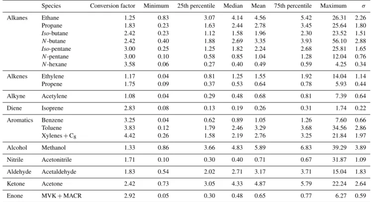
east-Table 1.Statistical summaries (µg m−3) of selected VOC concentrations measured at urban background sites. Statistics were calculated from hourly mean data, initially obtained every 30 min (ethane>isoprene) and every 5 to 10 min (for aromatics and OVOCs). These measurements were undertaken from 15 January to 22 November 2010 (∼10 months). A conversion factor is provided here to convert VOC concentrations (µg m−3) into (ppb) mixing ratios.
Species Conversion factor Minimum 25th percentile Median Mean 75th percentile Maximum σ
Alkanes Ethane 1.25 0.83 3.07 4.14 4.56 5.42 26.31 2.26 Propane 1.83 0.23 1.63 2.44 2.78 3.45 25.64 1.80 Iso-butane 2.42 0.23 1.12 1.58 1.96 2.30 23.52 1.51 N-butane 2.42 0.40 1.88 2.69 3.35 3.93 56.10 2.88 Iso-pentane 3.00 0.25 1.25 1.82 2.24 2.68 25.81 1.65
N-pentane 3.00 0.10 0.58 0.85 1.04 1.28 12.04 0.76
N-hexane 3.58 0.06 0.27 0.40 0.49 0.59 4.25 0.34
Alkenes Ethylene 1.17 0.04 0.81 1.25 1.55 1.92 14.04 1.14 Propene 1.75 0.09 0.37 0.53 0.64 0.78 5.93 0.44
Alkyne Acetylene 1.08 0.04 0.29 0.48 0.68 0.81 7.39 0.64 Diene Isoprene 2.83 0.08 0.13 0.19 0.26 0.31 1.74 0.22
Aromatics Benzene 3.25 0.04 0.62 0.89 1.05 1.26 7.60 0.66 Toluene 3.83 0.12 1.79 2.46 3.29 3.68 34.56 2.86 Xylenes+C8 4.42 0.26 1.58 2.19 2.76 3.25 21.84 1.97
Alcohol Methanol 1.33 0.86 3.66 4.83 5.89 6.83 39.29 3.89 Nitrile Acetonitrile 1.71 0.10 0.30 0.40 0.71 0.67 31.87 1.09
Aldehyde Acetaldehyde 1.83 0.54 2.02 2.71 3.17 3.71 15.04 1.83 Ketone Acetone 2.42 0.73 3.05 4.33 4.87 5.79 22.24 2.64
Enone MVK+MACR 2.92 0.05 0.30 0.48 0.65 0.77 6.27 0.59
ern France, the Benelux area, northern Germany and indica-tive of continental imports of long-lived pollutants (Gaimoz et al., 2011). Air masses coming from the west are gener-ally observed in summer and autumn (32–41 %), whereas northeast air masses are found to be significant in winter (34 %) and most frequently in spring (ca. 40 %), due to the stagnation of an anticyclone surrounding the British Isles (monthly weather report for Paris and its surroundings during April 2010, Météo-France) during that period.
3.2 VOC concentration levels in ambient air
The main results of descriptive statistics for all the mea-sured VOCs (from both GC-FID and PTR-MS instruments) on the whole sample set were summarized in Table 1. The average composition of VOCs was mainly characterized by oxygenated species (0.7–5.9 µg m−3 (0.4–4.4 ppb); 36.5 % of the TVOC mass), alkanes (0.5–4.6 µg m−3(0.1–3.7 ppb); 39.1 %) followed by aromatics (1.1–3.3 µg m−3; 16.9 % (0.3–0.9 ppb)) and to a lesser extent by alkenes, alkynes and dienes (0.3–1.6 µg m−3 (0.1–1.3 ppb); 7.5 %). Both alkanes and OVOCs significantly contribute up to 75 % of the TVOC concentrations. With ethane (10.9 %, 4.6 µg m−3 (3.7 ppb) on average) being the main alkane, methanol (14.0 %, 5.9 µg m−3 (4.4 ppb)) and acetone (11.6 %, 4.9 µg m−3 (2.0 ppb)) are considered to be the two major oxygenated
compounds measured in this study. This conclusion is in agreement with previous VOC measurements performed in downtown Paris in 2007 (Gros et al., 2011).
The comparison between these average ambient levels and VOC measurements reported in the literature for different ur-ban areas is restricted here to PTR-MS data as they consti-tute the most original dataset of this study. Most atmospheric studies were indeed conducted in urban metropolitan areas by investigating only NMHC measurements.
Table 2 summarizes PTR-MS data collected during the intensive experiment together with average VOC levels re-ported in ppb from other cities around the world. For the Paris megacity, a significant decrease in VOC concentrations was observed between spring 2007 and spring 2010 (from
−53.8 % for xylenes and C8aromatics to−25 % for benzene
and MVK+MACR+ISOPOOHs), except for methanol and
acetaldehyde (+11.8 %,+35.7 %, respectively). These
Table 2.Comparison of mean concentrations of selected VOCs (measured by PTR-MS) with ambient levels observed in the literature from different urban atmospheres. All average values are reported in parts per billion.
VOCs measured Parisa(P.) Parisb Barcelonac,1 Londond(P.) Mohalie(P.) Mexico Cityf(P.) Beijingg(P.) Houstonh(P.) by PTR-MS (m/z) Jan–Nov spring winter Oct May Mar Aug Aug–Sep
(spring)
2010 2007 2009 2006 (2010) 2012 (2010) 2006 (2010) 2005 (2010) 2000 (2010) Methanol (33.0) 4.5 (6.6) 5.9 NA NA (3.3) 38 (5.3) NA (1.6) 11.7 (2.8) 10.8 (3.9) Acetonitrile (42.0) 0.7 (1.2) 0.4 0.2–0.5 0.3 (0.2) 1.4 (0.5) 0.3–1.4 (0.2) NA (0.3) 0.5 (0.5) Acetaldehyde (45.0) 1.8 (1.9) 1.4 0.8–1.7 3.6 (1.5) 6.7 (1.7) 3.0–12.0 (1.1) 3.6 (1.1) 3.4 (1.5) Acetone (59.0) 2.1 (2.5) 3.0 1.1–1.6 1.6 (2.2) 5.9 (2.1) NA (1.7) 4.4 (1.6) 4.0 (2.1) MVK+MACR 0.2 (0.2) 0.3 0.07–0.12 NA (0.2) NA (0.1) NA (0.1) 0.3–0.6 (0.2) 0.8 (0.2)
+ISOPOOHs (71.0)
Benzene (79.0) 0.3 (0.3) 0.4 0.2–0.6 0.1 (0.4) 1.7 (0.3) NA (0.3) NA (0.2) 0.6 (0.3) Toluene (93.0) 0.9 (0.9) 1.4 0.8–2.7 1.9 (0.9) 2.7 (0.8) 3.0–28.0 (0.6) 1.0–4.0 (0.5) 0.8 (0.9) Xylenes+C8(107.0) 0.6 (0.6) 1.3 0.9–3.4 0.2 (0.7) 2.0 (0.7) NA (0.4) NA (0.4) 0.6 (0.6) aThis study (values in brackets from VOC measurements performed during the same sampling period of the other urban studies are given for comparison). (P.) denotes Paris.bGros et al. (2011). cSeco et al. (2013).dLangford et al. (2010).eSinha et al. (2014).fFortner et al. (2009) – values estimated from graphs.gShao et al. (2009).hKarl et al. (2003).1A full comparison was not possible because no data were available between 16 February and 24 March 2010. NA: non-available data.
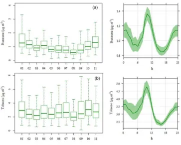
Among selected species, benzene (as a carcinogenic agent) is one of the few regulated VOCs. According to the direc-tive 2000/69/EC (2000), the annual mean benzene concen-tration in ambient air should not exceed 5 µg m−3(1.5 ppb). Background levels of benzene were relatively stable in recent years, with an annual average concentration of 1.1 µg m−3 (0.3 ppb) (Airparif, 2015).
Average VOC concentrations were also calculated in line with sampling periods of the other European and global stud-ies over different years (see Table 2). In this study, measured VOC levels were in the range of those found within some European cities (Barcelona and London – from 0.1 to 2.1 ppb concentration differences). However, average VOC levels ob-served in Paris were significantly lower than those measured in Houston (USA – from 0.1 to 6.9 ppb concentration differ-ences) and more particularly in Beijing (China – from 2.5 to 8.9 ppb), in Mexico City (Mexico – from 0.1 to 27.4 ppb) and in Mohali (India – from 0.9 to 32.7 ppb).
3.3 Seasonal and diurnal variations
The variability in VOC concentration levels is controlled by a combination of factors including source strengths (e.g., emissions), dispersion and dilution processes as well as pho-tochemical reaction rates with OH radicals and other ox-idants (Filella and Peñuelas, 2006). Variations of selected trace gases (nitrogen/carbon monoxide, NO/CO – Fig. 6)
and VOCs illustrating contrasting emission sources and at-mospheric lifetimes were analyzed at different timescales. As (O)VOCs measured by PTR-MS constitute the most original data of this study (and represent∼37 % of the TVOC mass);
a discussion on their variations (Fig. 7) and their respective sources is given here. For information, an overview of sea-sonal and diurnal profiles of lighter hydrocarbons (C2–C6) measured by GC-FID is reported in Sect. S6 in the Supple-ment.
Figure 6.Left: monthly box and whisker plots of NO(a)and CO(b) expressed in µg m−3 and ppb, respectively. Solid lines represent the median concentration and the box shows the interquartile range (IQR). The bottom and top of the box depict the 25th (the first quar-tile) and the 75th (the third quarquar-tile) percentile. The ends of the whiskers correspond to the lowest and highest data still within 1.5 times the IQR of Q1 and Q3, respectively. Right: diurnal variations of NO and CO averaged over the whole sampling period. Time is given as local time. Lines correspond to hourly means and shaded areas indicate the 95 % confidence intervals of the mean.
Known as combustion tracers (traffic/wood-burning),
mix-Figure 7.
ing compared to the other seasons. Another explanation of this variability is the increase in NO and CO emissions due to home heating fuels consumed in winter. NO concentra-tions are significantly enhanced between 06:00 and 12:00 LT (with the maximum around 09:00 LT). Contrary to NO, the diurnal pattern of CO is characterized by a double wave profile with an initial peak at 07:00–10:00 LT (maximum at 09:00 LT) and a second one at the end of the afternoon be-tween 16:00 and 21:00 LT. These increases typically corre-spond to morning and evening rush-hour traffic periods, as previously observed in Ammoura et al. (2014). The evening peak is smaller in magnitude than the morning one partly due to a higher planetary boundary layer (PBL) height in the afternoon (leading to dispersion and dilution processes) and to more disperse traffic periods. After 21:00 LT, CO levels stay quite high (240–260 ppb) due to several factors: ongoing emissions (traffic and wood-burning activities), lower photo-chemical reactions and atmospheric dynamics (the shallower boundary layer leads to more accumulation of CO (and other co-emitted species)). The evening event is not observed for NO as during this time ozone (O3) presents its highest con-centrations, leading to the titration of NO.
Good correlations between CO and some alkanes (iso-/n
-pentane, n-hexane), alkenes (ethylene, propene), acetylene
and aromatics (benzene, toluene and xylenes plus C8) were found when considering a Pearson’s correlation coefficientr
greater than 0.6. All these compounds follow a similar sea-sonal and diurnal pattern, indicating that they share some or almost all common sources related to anthropogenic com-bustion processes (e.g., road traffic and/or wood-burning). These observations are in agreement with the conclusions from Gros et al. (2011) and Gaimoz et al. (2011).
With atmospheric lifetimes from a few hours to several days, oxygenated species (OVOCs) are emitted from pri-mary sources, mainly of biogenic origins, and significant
secondary sources related to the oxidation of hydrocarbons. High concentration levels of OVOCs (for instance, methanol) and CO were observed during winter months (the season with coldest temperatures and where wood-burning-related activities can play an important role). The low height of the PBL is also a relevant factor to consider as it can lead to the stagnation and the accumulation of VOC species into the tro-posphere during that season. In addition, significant OVOC levels were observed from April to September. In springtime, elevated baseline levels were measured when the Paris region was mostly influenced by northeast influences (see Fig. 5), suggesting that they partly depended on continental imported and already processed air masses. Biogenic emissions indeed contributed to high OVOC concentrations during this season and in summer.
Methanol is usually released into the atmosphere by veg-etation and man-made activities contributing to a relatively high background levels during most of the year. This com-pound displays a specific diurnal pattern depending on the season and atmospheric dynamics (see Sect. S4 in the Sup-plement). In winter, methanol shows a double wave pro-file with two peaks at 10:00–11:00 and 19:00–20:00 LT (see Fig. 7c, bottom left), suggesting the influence of anthro-pogenic activities (e.g., road traffic, wood-burning sources). A slight delay (1–2 h) is observed for methanol in compar-ison to other primary species (for instance, aromatics). In summer, methanol is characterized by high concentrations during night hours (00:00–06:00 LT), followed by a signif-icant decrease until the early afternoon and another increase from 18:00 LT to midnight (Fig. 7c, bottom right). This nighttime maximum of methanol has already been observed in urban environments, however, with no clear explanation (Solomon et al., 2005). This diurnal cycle can possibly be in-terpreted as the accumulation of species concentrations dur-ing the night from a local source under a shallow inversion layer, which is decreasing when the PBL is increasing (as di-lution and dispersion processes are occurring). However, the corresponding nighttime source has not been yet identified.
With a relatively short lifetime (∼9 h), acetaldehyde
shows a diurnal cycle fairly comparable to acetone (Fig. 7d, e). Lower concentrations were observed during the night and from 18:00 LT. Average levels increase from sunrise to a maximum at noon and slightly decrease in the after-noon. For these two OVOC species, the reduction of con-centrations does not occur in the same way. From 12:00– 18:00 LT, average acetaldehyde concentrations are linearly decreasing (∼1.0 µg m−3 or 0.5 ppb) while mean acetone
levels show a slower decline rate (∼0.5 µg m−3or 0.25 ppb)
with a tiny raise at 17:00 LT. This finding depends on their emission sources and strengths (e.g., biogenic, sol-vent use), but also on their respective photochemical reac-tion rates (1.5×10⁻¹¹cm3molecule−1s−1for acetaldehyde
and 1.8×10⁻¹³cm3molecule−1s−1for acetone) (Atkinson
et al., 2006). As acetone has a relatively long atmospheric
lifetime (∼68 days), concentration levels are often more
ho-mogeneous.
Finally, methyl vinyl ketone, methacrolein and isoprene hydroxy hydroperoxides (MVK+MACR+ISOPOOHs),
three secondary products of isoprene photo-oxidation (as good indicators of biogenic activities), exhibit high levels in the late afternoon due to the oxidation of daytime isoprene. The formation of these compounds mostly occurs in summer, but also in winter (Fig. 7f). This fact could eventually be re-lated to anthropogenic activities such as wood-burning (see Sect. 2.4.2, Fig. 3).
3.4 Source apportionment
3.4.1 Motor vehicle exhaust factor
The speciation profile of Factor 1 (see Fig. 8a) exhibits high contributions of alkanes, such as pentanes (iso-/n-)
and n-hexane with on average ∼50 % of their
variabili-ties explained by this factor. Aromatic compounds (toluene, xylenes plus C8, benzene;∼35 %) and light alkenes
(ethy-lene, propene), which are considered as typical combustion products, are also the predominant species in this factor.
To evaluate the relevance of this factor, a compari-son between speciated profiles from tunnel measurements (Fig. 2) and PMF simulations was done and is reported in Fig. 9. Traffic profiles are in general coherent and consistent amongst themselves, thus allowing to label this factor as a motor vehicle exhaust source. Indeed, a good agreement is observed between these two profiles for the major species such as iso-/n-pentane, toluene, ethylene and propene.
Figure 8.Source composition profiles of the six-factor PMF solu-tion. The concentrations (µg m−3) and the percent of each species apportioned to the factor are displayed as a pale blue bar and a color box, respectively.(a)F1 – motor vehicle exhaust;(b)F2 – evapo-rative sources;(c)F3 – wood-burning;(d)F4 – biogenic;(e)F5 – solvent use;(f)F6 – natural gas and background.
of the mixed natural gas and background source (for which ethane contributions seem to be underestimated).
Factor 1 displays fair correlations with nitrogen monox-ide/dioxide (NO/NO2), carbon monoxide (CO) and black carbon (from its fossil fuel fraction), which are known to be relevant vehicle exhaust markers (0.53< r <0.64). The
average contribution of this factor is rather stable through-out the year (5.8 µg m−3; see Fig. 10, panel 1 and Sect. S7 in the Supplement). A smaller contribution is found dur-ing winter (3.2 µg m−3), whereas the highest emissions from motor vehicle exhaust occur in autumn (8.6 µg m−3 on av-erage) with a contribution of up to 10.1 µg m−3 in Septem-ber. This seasonal cycle has already been observed and de-scribed in Bressi et al. (2014) for the road traffic source of fine aerosols in Paris. The diurnal variation of this source is characterized by a double wave profile with an initial in-crease at 07:00–10:00 LT and a second inin-crease at the end of the afternoon between 16:00 and 19:00 LT. These
in-Figure 9.Comparison of speciated profiles issued from the high-way tunnel experiment and PMF simulations (F1 – motor vehi-cle exhaust). The species contributions are expressed in percent. NF=near-field.
creases correspond to morning and evening rush-hour traf-fic periods. After 21:00 LT, the absolute contributions of this factor stay quite high (7.0–8.0 µg m−3) due to several factors: ongoing emissions (until midnight), lower photo-chemical reactions and atmospheric dynamics (the shallower boundary layer leads to more accumulation of pollutants at night). Lower contributions are generally displayed during late mornings/early afternoons and at night. This reduction in factor contributions could be mainly explained by dilution and OH oxidation processes of more reactive species, which are not being balanced by additional vehicular emissions. This pronounced cycle has already been reported in previ-ous studies (Gaimoz et al., 2011, and references therein). The temporal source strength variation is usually much more pro-nounced during weekdays than the weekend.
3.4.2 Evaporative sources factor
The profile of Factor 2 (see Fig. 8b) exhibits a high con-tribution from propane andiso-/n-butanes, with more than
47 % of their variabilities explained by this factor. It was al-ready identified by Gaimoz et al. (2011) and is used here as reference profile from gasoline evaporation emissions (in-cluding storage, extraction and distribution of gasoline or liquid petroleum gas (LPG)). The generic term “evaporative sources” is here used to take into account these types of evap-orative emissions. Factor 2 also includes a significant propor-tion of isoprene (20 %). This finding is still consistent with the conclusions of Borbon et al. (2001), which have shown that traffic activities emit a small amount of isoprene. In the same way, oxygenated compounds (acetaldehyde (4 %), ace-tone (6.6 %)) were found in fugitive evaporative emissions in agreement with what was observed during the highway tun-nel experiment (see Fig. 2).
Among independent tracers used, only NO displays a fair agreement with this factor (r=0.35). A correlation between
F2 and F1 can also be noted (r=0.36), thus indicating that
Figure 10.
traffic). This source is in the range of∼3.9 µg m−3over the
whole studied period (see Fig. 10, panel 2). The annual trend of F2 seems to be consistent with the motor vehicle exhaust factor (F1), even though its monthly change remains ambigu-ous. Indeed, lower evaporative contributions are recorded both in winter and in early summer with minimum average contributions in June and July (1.7 µg m−3). This finding was already identified by Frachon (2009). However, this value in June is somewhat puzzling as road traffic emissions are usu-ally significant (4.9 µg m−3). In July, propane and butanes (iso-/n-) values were missing due to analytical problems on
the operating GC-FID. Consequently, these compounds were simulated by the PMF model (e.g., missing values were vir-tually substituted by median values) which may underesti-mate the contribution of this factor during this specific pe-riod of time. However, high contributions of this source oc-cur in August (6.6 µg m−3). Although exhaust emissions are not particularly important, this observation could be eventu-ally explained by gasoline storage and distribution sources,
Figure 10.Left: monthly box and whisker plots of modeled sources from the six-factor solution. Concentration levels are expressed in µg m−3. Solid lines represent the median concentrations and the box shows the IQR. The bottom and top of the box depict the 25th (the first quartile) and the 75th (the third quartile) percentile. The ends of the whiskers correspond to the lowest and highest data still within 1.5 times the IQR of Q1 and Q3, respectively. Right: diurnal varia-tions of the resolved PMF factors. Time is given in local time. Lines correspond to hourly means and shaded areas indicate the 95 % con-fidence intervals of the mean.
which may have increased with higher temperatures during that month. Maxima temperatures have generally been in the range of 16 to 32◦C. The source contribution is on average higher in autumn (6.1 µg m−3) with a contribution of up to 6.3 µg m−3in October.
The diurnal variation of this factor contribution is charac-terized by a nighttime minimum, an increase from 07:00 to 10:00 LT (consistent with the motor vehicle exhaust factor, F1) and a much slower decrease in emissions during the after-noon than those observed for the vehicle combustion profile. This second factor therefore represents the emissions of less reactive species (OVOCs, propane, butanes), for which con-centrations cannot be expected to be consumed photochem-ically in short transport times. The temporal source strength variation is less pronounced on weekends than weekdays, which is typical of mobile source activity patterns.
hot soak reactions (when a hot engine is switched off). It was speculated that hot engines would emit more in the morning than in the evening, considering typical conditions of active inhabitants going to and from their workplace. Fugitive gaso-line emissions from the loading of tank trucks, transportation and unloading from tank trucks at service stations and dis-tributions depots can also be likely sources of this factor. In summary, this source depends on several parameters (related to road traffic conditions, the vehicle fleet composition, eco-nomic activities and meteorological observations), which can make the interpretation of its seasonal variability difficult.
3.4.3 Wood-burning factor
In Paris, domestic wood-burning represents a non-negligible part (about 5 %) of the energy consumption by fuel used for home heating (Airparif, 2011). The chemical profile of this source (Factor 3), shown in Fig. 8c, is mainly dominated by acetylene with approximately 80 % of its variability ex-plained by this factor. It also includes ethylene (57.4 %), ben-zene (22.7 %) and oxygenated compounds, such as acetoni-trile, acetaldehyde and methanol (with 18.3, 12.6 and 8.2 %, respectively). Acetonitrile is a hydrocarbon commonly used as a marker of biomass burning (Holzinger et al., 1999). All these chemical species typically reflect an anthropogenic source related to wood combustion processes (Lanz et al., 2008; Leuchner et al., 2015) in agreement with the fireplace emission profile (see Sect. 2.4.2, Fig. 3). No full compari-son between both speciation profiles was possible as the fire-place profile was based on a limited number of data. With this mind, only a qualitative approach allowed to identify predominant species emitted from this source and confirm the term “wood-burning” assigned to this factor.
Biomass burning emissions are well correlated with black carbon originating from residential wood-burning (BCwb) and carbon monoxide, a long-lived compound especially emitted from combustion reactions (0.6< r <0.7). In
addi-tion, they co-vary well with naphthalene (m/z129.0
mea-sured by PTR-MS), a known polyaromatic hydrocarbon emitted from combustion processes (industry, tailpipe emis-sions) including wood-burning (Purvis and McCrillis, 2000). As expected, wood-burning contributions display a distinct cycle with a winter maximum (20.5 µg m−3on average) and a summer minimum (3.3 µg m−3). Average contributions of this factor are rather stable in both spring and fall (6.9 and 5.9 µg m−3, respectively).
Wood-burning emissions linked to home/building heating are obviously highly dependent on meteorological conditions and particularly on cold temperatures. A clear negative rela-tionship between the wood-burning factor and temperature is found (r= −0.56). The diurnal variation of this source
ex-hibits a double wave profile. Average contributions increase from sunrise to a maximum in midmorning and decrease un-til 16:00–17:00 LT. At the end of the day, a second increase is observed with another maximum contribution at 19:00–
21:00 LT. This diel cycle can be explained by domestic be-haviors. An important finding is that the diurnal pattern of this source is fairly comparable to that of the motor vehicle exhaust factor. However, the wood-burning factor does not display any distinct weekly variation. High contributions are observed all week (without any distinction between week-days and weekends) compared to motor exhausts, for which vehicular emissions are less pronounced on weekends than weekdays. In addition, it exhibits poor correlations with NO, NO2 and BCff (r=0.30, 0.29 and 0.19, respectively), thus
indicating that the wood-burning factor is completely inde-pendent of the motor vehicle exhaust source.
3.4.4 Biogenic factor
The profile of Factor 4 (see Fig. 8d) exhibits a high con-tribution from isoprene, a known chemical marker of bio-genic emissions, with more than 79 % of its variability ex-plained by this factor. In addition, this factor profile in-cludes isoprene’s oxidation products (methyl vinyl ketone (MVK), methacrolein (MACR) and isoprene hydroxy hy-droperoxides (ISOPOOHs)), methanol and acetone. These oxygenated compounds have a large contribution from bio-genic emissions (Kesselmeier and Staudt, 1999; Guenther, 2002). It also accounts a significant contribution of some light alkenes (e.g., ethylene and propene), which can be evenly emitted by plants (Goldstein et al., 1996). Conse-quently, this factor F4 is termed “biogenic factor”. Amounts of light alkanes (butanes,iso-pentane,n-hexane) and
acetoni-trile were also found in this profile and could be attributed to a mixing with other temperature-related sources or artefacts from the PMF model (Leuchner et al., 2015).
Biogenic emissions are directly related to solar radia-tion (Steiner and Goldstein, 2007) and ambient temperature (r >0.7). For that reason, the highest biogenic factor
con-tributions occur in summer (10.5 µg m−3on average) with a contribution of up to 14.3 µg m−3 in July. Daily mean con-tributions gradually increase from 09:00 LT. A slight delay is observed in comparison with diurnal temperature/solar radiations variations (for which values increase from sun-rise at 06:00 LT). We assume that chemistry affects this fac-tor as it takes part in the formation of secondary species (MVK+MACR+ISOPOOHs, for instance) from the
3.4.5 Solvent use factor
The profile of Factor 5, shown in Fig. 8e, is associated with a large contribution of selected OVOCs (acetaldehyde, methanol and acetone) with on average∼33 % of their
vari-abilities explained by this factor. Significant contributions from aromatic compounds (toluene, xylenes plus C8and ben-zene) and some alkanes (pentanes, butanes, propane andn
-hexane) are also observed. Toluene, in addition to road traf-fic, is a good marker for solvents originating from an indus-trial source (Buzcu and Fraser, 2006). Benzene, due to its toxic and carcinogen nature, was regulated in recent years and was strongly limited in solvent formulations. Current standards establish limits in benzene concentrations at 0.1 % in cleaning products. However, PMF results point out the presence of benzene in this factor, suggesting that this com-pound might potentially still be in use by some manufactur-ers. Finally, the presence of these aforementioned species il-lustrates that this profile could be linked to industrial emis-sions, although a mixing of different sources cannot be ex-cluded.
This factor co-varies well with ethanol, butan-2-one (also called methyl ethyl ketone – MEK), isopropyl alcohol or even ethyl acetate (0.68> r >0.52, respectively) – four
or-ganic compounds that were measured by GC-MS during the MEGAPOLI campaign (January–February 2010). These species are often used as solvents, diluents or cleaning fluids in industrial processes (Zheng et al., 2013). Some manufacto-ries can consume fossil fuels for their activities, which may explain the fairly good correlation between this factor and black carbon originating from fossil fuels (BCff,r=0.50).
Indeed, these fossil fuels could be used by industries as di-verse as paints, paintings inks and lacquers (Tsai et al., 2001; Cornelissen and Gustafsson, 2004).
The highest contribution of this factor is observed dur-ing winter (14.2 µg m−3) with a contribution of up to 15.5 µg m−3 in January. In winter, factor contributions in-crease at 06:00 and reach their maximum between 11:00 and 19:00 LT (15–20 µg m−3) before a long and gradual decline in the evening (see Fig. 10, panel 5 – top right). Higher con-tributions in winter can be explained by lower photochemi-cal reactions (combined with weaker OH concentrations/UV radiations) and atmospheric dynamics. Indeed, a shallower PBL (and consequently, less intense vertical dynamics) leads to more accumulation of pollutants and thus to higher source contributions. The daily wintertime variability of this source is in agreement with the diel cycle of independent tracers (ethanol, butan-2-one).
Reconstructed contributions associated with this factor are also significant in summer (12.6 µg m−3in July), which could be mainly explained by the evaporation of solvent inks, paints and other applications during that month due to higher temperatures. In spring/summer/autumn, factor con-tributions also increase at sunrise, but reach their maximum between 08:00 and 10:00 LT (typical of anthropogenic
activ-ities). They progressively decrease during the afternoon (see Fig. 10, panel 5 – bottom right). This gradual decline (not earlier observed in winter) is influenced by greater photo-chemical reactions and more intense vertical dynamics dur-ing these three seasons, leaddur-ing to dispersion and dilution processes (and consequently, lower source contributions dur-ing the afternoon).
The temporal source strength variation is much more pro-nounced during weekdays than the weekend, except on Sat-urday morning. These diel and weekly patterns seem to be consistent with industrial source activities.
3.4.6 Natural gas and background factor
The profile of Factor 6, shown in Fig. 8f, is mainly dominated by ethane with around 45 % of its variability explained by this factor. It also contains propane (14.7 %) and light alka-nes (butaalka-nes), which are key long-lived compounds known to be associated with natural gas leakages. Such species have already been identified in the natural gas experiment (see Sect. 2.4.2, Fig. 4), thus allowing to confirm the identification of this profile. The diel pattern of this factor is mainly based on the diurnal variation of ethane, which is characterized by a nighttime maximum and a midafternoon minimum. Mainly due to its low reactivity, the behavior of ethane can be inter-preted as homogeneous species levels during the night under a shallow inversion layer, then followed by concentration re-ductions caused by the increase of the PBL and vertical mix-ing – leadmix-ing to dispersion and dilution processes. Average contributions of this factor were significantly higher when the PBL was low (∼11.0–14.0 µg m−3) and lower when the
PBL was high (∼6.0 µg m−3).
This F6 profile is also characterized by the presence of ox-idized pollutants (OVOCs including acetone and methanol) and aromatic compounds (like benzene), which have rela-tively long atmospheric residence times of respecrela-tively 53, 12 and 9 days (assuming OH=2.0×10⁶molecules cm−3)
(Atkinson, 2000). Because of their low reactivity, all the species of this factor tend to accumulate in the atmosphere and show significant background levels, especially in the Northern Hemisphere. The resulting emissions can be con-sidered as a partly aged background air, implying a possible regional background and/or a long-range (intercontinental) transport.
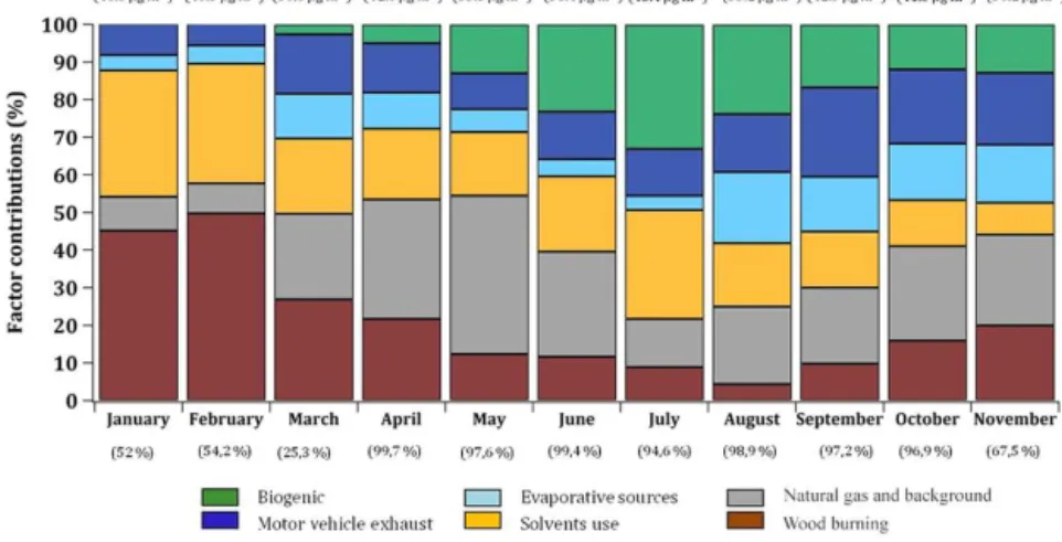
Figure 11.Variations of monthly averaged contributions of the six modeled VOC sources (expressed in percent); (top) average predicted VOC concentration levels per month (µg m−3); (bottom) completeness of the data per month (%).
wood-burning factors. Consequently, we supposed that the natural gas and background factor contributions were under-estimated (especially in winter) for the benefits of the wood-burning factor (another source significantly contributing dur-ing this season).
The highest contributions occur in spring (13.3 µg m−3) when the Paris region is mostly influenced by prevailing air masses originating from the north and the northeast parts of Europe passing over Germany and the Benelux area (see Fig. 5). These continental imports constitute background events, which significantly impact baseline levels of ethane and oxygenated species. Slightly lower reconstructed mass contributions of this factor F6 were also observed in autumn. This fact can be explained by the consumption of natural gas (for home heating) during this season as average tempera-tures are progressively going down. No significant continen-tal influences occur during the fall period as main air masses are coming from the west, south and southeast sectors, thus illustrating the importance of local pollution emissions dur-ing this season.
3.5 VOC source contributions
PMF simulations revealed the significant contribution of six VOC emission sources (e.g., five specific factor profiles and a mixed one, for which the natural gas source could not be isolated from background emissions). This source apportion-ment (SA) analysis concluded that the predominant sources at the receptor site were road traffic-related activities (in-cluding motor vehicle exhaust, with 15 % of the TVOC mass on the annual average, and evaporative sources, with 10 %), with the remaining sources from natural gas and background (23 %), solvent use (20 %), wood-burning (17 %) and bio-genic activities (15 %). Each modeled factor exhibits distinct patterns due to the variations of the different source emis-sions and meteorological conditions. Monthly averaged con-tributions (expressed in percent) of these factors to TVOC
mass are reported in Fig. 11. Seasonal variations of the in-dividual sources have already been discussed in the previous sections. Therefore, only the most important features are re-ported here.
Road traffic emissions were identified by PMF simulations to be the main source of VOCs in Paris. The sum of mo-tor vehicle exhaust and evaporative source contributions ac-counted for a quarter of the TVOC mass. It showed higher contributions at the end of the year (21 and 15 %, respec-tively), which is still consistent with the study from Bressi et al. (2014) and with long-term black carbon measurements (Petit et al., 2015) linked to enhanced traffic during autumn in Paris. Most importantly, it was observed that the wood-burning source exhibited a significant contribution in winter months (almost 50 % in January and February), which is still in agreement with wood-burning-related particle emissions (Favez et al., 2009). The biogenic source also displayed a significant contribution (∼30 %) in summer (mainly due to
the weight of oxygenated species in the factor profile). The solvent use source displayed high contributions during winter months (∼33 %, due to a lower PBL height and slower
pho-tochemical reactions during that period) and in July (due to the evaporation of solvents controlled by temperature). The source mixing natural gas and background showed a higher proportion in springtime (∼34 %) and lower proportions
dur-ing autumn (∼25 %). This conclusion can be explained by
pollution events that are both related to air masses imported from continental Europe (see Fig. 5) and/or specific meteo-rological conditions (low temperatures involving the use of home heating), respectively.