Intraperitoneal Glucose Sensing is Sometimes
Surprisingly Rapid
A.L. Fougner1 2 K. K¨olle1 2 N.K. Skjærvold3 4 N.-A. L. Elvemo5 D.R. Hjelme6 R. Ellingsen6 S.M. Carlsen4 7 Ø. Stavdahl1
1
Dept. Engineering Cybernetics, Norwegian University of Science and Technology (NTNU), Trondheim, Norway 2
Central Norway Regional Health Authority, Trondheim, Norway 3
Dept. Circulation and Medical Imaging, NTNU, Trondheim, Norway 4
St Olavs Hospital, Trondheim, Norway 5
GlucoSet AS (NO 997 780 922) 6
Dept. Electronics and Telecommunication, NTNU, Trondheim, Norway 7
Dept. Cancer Research and Molecular Medicine, NTNU, Trondheim, Norway
Abstract
Rapid, accurate and robust glucose measurements are needed to make a safe artificial pancreas for the treatment of diabetes mellitus type 1 and 2. The present gold standard of continuous glucose sensing, subcutaneous (SC) glucose sensing, has been claimed to have slow response and poor robustness towards local tissue changes such as mechanical pressure, temperature changes, etc. The present study aimed at quantifying glucose dynamics from central circulation to intraperitoneal (IP) sensor sites, as an alternative to the SC location.
Intraarterial (IA) and IP sensors were tested in three anaesthetized non-diabetic pigs during experi-ments with intravenous infusion of glucose boluses, enforcing rapid glucose level excursions in the range 70–360 mg/dL (approximately 3.8–20 mmol/L). Optical interferometric sensors were used for IA and IP measurements. A first-order dynamic model with time delay was fitted to the data after compensating for sensor dynamics. Additionally, off-the-shelf Medtronic Enlite sensors were used for illustration of SC glucose sensing.
The time delay in glucose excursions from central circulation (IA) to IP sensor location was found to be in the range 0–26 s (median: 8.5 s, mean: 9.7 s, SD 9.5 s), and the time constant was found to be 0.5–10.2 min (median: 4.8 min, mean: 4.7 min, SD 2.9 min).
IP glucose sensing sites have a substantially faster and more distinctive response than SC sites when sensor dynamics is ignored, and the peritoneal fluid reacts even faster to changes in intravascular glucose levels than reported in previous animal studies.
This study may provide a benchmark for future, rapid IP glucose sensors.
Keywords: Diabetes, Artificial Pancreas, Closed-loop systems, Type 1 diabetes, Type 2 diabetes.
1 Introduction
Glucose concentration can in principle be measured in all tissues. While intraarterial (IA) and intravenous (IV) measurements are not practically usable in outpa-tients, subcutaneous (SC) sensing has become the stan-dard for continuous glucose monitoring (CGM) during
indicate that novel CGM systems may be less prone to such problems (Garcia et al.,2013;Bailey et al.,2015). These challenges originate partly from the sensor tech-nology and partly from the physiologically slow glucose transfer between intravascular glucose levels and glu-cose levels in subcutaneous tissue.
Intraperitoneal (IP) glucose sensing seems to offer faster dynamics (including shorter time delays) than SC sites (the termdynamics/system dynamics is here-after used synonymously with what has previously been denotedkinetics, e.g. by Burnett et al. (2014)). Additionally, an IP sensor location may be less prone to mechanical disturbances (Helton et al.,2011;Mensh et al.,2013), variation due to fluctuation in tissue per-fusion (Cengiz and Tamborlane, 2009; Burnett et al., 2014; Stout et al., 2004) and temperature effects as the body core temperature is strictly regulated. Thus, based on previous animal studies, the peritoneal cavity is a promising alternative location for continuous glu-cose sensing (Burnett et al., 2014; Clark et al., 1987, 1988;Velho et al.,1989).
Figure 1: The GlucoSet sensor (Tierney et al., 2009; Skjærvold et al.,2012).
1.1 Objectives
The aim of the present study was to (A) assess whether interferometric sensors can be used to measure in-traperitoneal (IP) glucose levels, and to (B) quantify how fast the glucose dynamics are from central circula-tion to IP sensor sites. We consider (B) to be the most important of these, but (A) is a requirement in order to perform (B).
2 Methods
The study was approved by the Norwegian Animal Re-search Authority (FOTS approval id 6538).
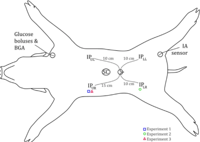
10 cm
IP 10 cm
10 cm 15 cm
SC
IA sensor
UL
IPLR IPLL
IPUR Glucose
boluses & BGA
Experiment 1 Experiment 2 Experiment 3
Figure 2: Approximate sensor placement and other in-strumentation on the animal (BGA = blood gas analysis; IP = intraperitoneal; IA = in-traarterial; SC = subcutaneous, UL = up-per left quadrant, UR = upup-per right quad., LL = lower left quad., LR = lower right quad.). The working IP sensors for each ex-periment is indicated with symbols. The fig-ure is licensed under a Creative Commons BY-NC-SA 4.0 license (hereafter abbreviated to Copyright: CC BY-NC-SA 4.0).
2.1 The animal model
Three healthy, young farm pigs, weight 25–30 kg, were enrolled in the study and used in one experiment each, hereafter named experiment 1, 2 and 3. The animals were anaesthetized and euthanized as described in ear-lier studies (Skjærvold et al., 2012, 2013). A central venous line was established via the left internal jugular vein and an arterial line via the left external carotid artery, respectively, for monitoring, glucose bolus ad-ministration and blood sampling.
2.2 Sensors
A modification of the original 3APB-alpha was used in one experiment, hereafter referred to as “3APB-beta”. This modified sensor has slower dynamics but is more robust to other constituents of the measured fluid. De-tails on the specific composition are proprietary to the sensor manufacturer.
Enzyme-based amperometric Enlite sensors from Medtronic (Medtronic PLC, Dublin, Ireland) were used for SC glucose measurements, since the GlucoSet sen-sors cannot be used subcutaneously. These sensen-sors were used only for illustration purposes, as their data was too sparse for system identification in the short segments analysed (offering values only every 5 min-utes).
Blood samples from the external carotid artery were used for reference glucose measurements and analysed on a Radiometer ABL 725 blood gas analyser (Ra-diometer Medical ApS, Brønshøj, Denmark). During experiment 1, these samples were taken mostly in sta-ble periods (i.e. before each glucose bolus). During experiment 2 and 3, blood samples were taken more frequently, especially after each glucose bolus, in order to verify the IA glucose level excursions.
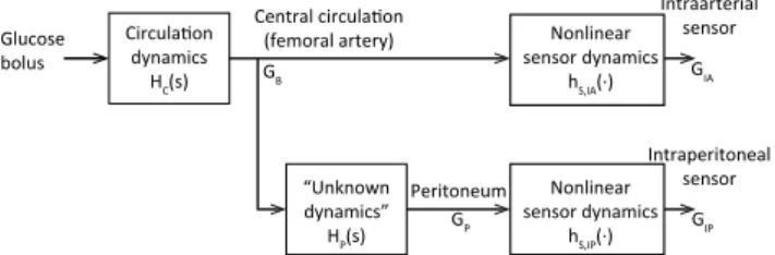
GIA
GIP GB
Glucose bolus
Intraperitoneal sensor Intraarterial
sensor
Central circulaion
(femoral artery)
Circulaion
dynamics HC(s)
Nonlinear sensor dynamics
hS,IA(·)
Nonlinear sensor dynamics
hS,IP(·) “Unknown
dynamics”
HP(s) GP
Peritoneum
Figure 3: Model of glucose dynamics from infusion site to sensor sites, where GB(t) is the blood glu-cose concentration; GP(t) is the peritoneal fluid (or peritoneal lining) glucose concentra-tion; GIA(t) is the intraarterial (IA) sensor signal; GIP(t) is the intraperitoneal (IP) sen-sor signal; HC(s) is the circulation dynam-ics (from jugular vein to the femoral artery); HP(s) is the unknown physiological dynam-ics (from the femoral artery to the peritoneal sensor site); and hS,IA(·), hS,IP(·) are the
non-linear sensor dynamics in IA and IP sensors, respectively. Copyright: CC BY-NC-SA 4.0.
2.3 Sensor placement
The intention was to use one IA and one IP sensor in each experiment. However, a larger pool of sen-sors was used in order to have some in backup, since the interferometric sensors are susceptible to damage during insertion. Additionally, the IP sensor response can vary between different locations in peritoneum, so
they were directed in four different angles from the in-sertion. Some sensors were corrupted by noise or other artifacts to the point where the glucose boluses were completely obscured and were thus not interpreted as a measure of glucose levels (hereafter called “noninter-pretable sensors”). In the end only one IA and one IP sensor worked in each experiment, so a complete ana-lysis of sensor location was not carried out. See also the discussion in Section4.
Approximate sensor placement is shown in Fig-ure2. IP glucose sensors were inserted through a mini-laparotomy in the ventral midline a few centimetres below the umbilicus, and the sensors were directed to-wards different IP positions. IA glucose sensors were inserted through the superficial part of the femoral artery after minimal surgical cut-down, either bilater-ally (experiment 1 and 2) or uni-laterbilater-ally (experiment 3). In experiment 1, one 3APB-alpha sensor and one beta sensor were tested, but only the 3APB-alpha signal was used for system identification (see Sec-tion 2.5.2). In experiment 2, the 3APB-alpha sensor was damaged during insertion, so only the 3APB-beta sensor was used. In experiment 3, one 3APB-alpha sensor was used.
During experiment 1, two IP sensors were inserted, but one of them was damaged during insertion, so only one IP sensor worked (15 cm into the upper right quad-rant, see Figure 2). Accordingly, in experiment 2, the number of IP sensors was increased to four. All sensors gave readable signals, but only one of them (10 cm into lower right quadrant) could be interpreted as a mea-sure of glucose levels. The signals from the remaining sensors were deemed noninterpretable.
During experiment 3, three IP sensors were inserted. It was decided to move/pull on the sensors to see if a new position or a change to the sensor surroundings influenced the signal. One sensor (15 cm into the up-per right quadrant) worked during the whole exup-peri- experi-ment, but dynamics were changed after pulling it 1 cm between bolus segments C and D (see Section 3 and Table 1). The other two sensors, placed 15 cm into the lower and upper left quadrants, respectively, did not give usable signals even after moving them to new locations (one was moved to the lower right quadrant) or pulling them 1–5 centimetres. These were deemed noninterpretable.
All disturbances (e.g. unintentionally touching a sensor cable) were recorded, in order to be able to in-terpret the signals and noise.
SC sensors were placed according to manufacturer’s instructions in the ventral midline approximately five centimetres above the umbilicus.
2.4 Glucose bolus administration
Glucose boluses were administered as 2, 4 and 8 mL of glucose 500 mg/mL (B. Braun, Melsungen, Ger-many), yielding boluses of 1, 2 and 4 g or 5.5, 11.1 and 22.2 mmol. The boluses were injected into the external jugular vein within 2—3 seconds and the catheter was immediately flushed with 10 mL of NaCl 9 mg/mL. Boluses were injected 10-–20 minutes apart.
The first glucose bolus of each trial was initiated only after completion of SC sensor calibration and insertion of IP sensors.
As the last part of each experiment, glucose was in-jected in series of 3–4 boluses with approximately two minutes in between.
2.5 Synchronization and data handling
Every recorded action, such as glucose boluses or blood sampling, was time stamped. During start-up of each experiment, a synchronization procedure was per-formed. Since the SC sensor read-out unit (Medtronic Guardian Real-Time CGM) does not indicate seconds, timestamps from all other sensors were taken when the minute indicator incremented on the Medtronic device, yielding second-level synchronization across the differ-ent devices.
Before system identification, data was segmented so that each segment started with a glucose bolus and ended before the next known bolus or recorded distur-bance. Hereafter, segments are named by combining the experiment number (1—3) with capital letters, e.g. segment 3F representing “experiment 3, segment F”. Segments with interruptions too soon after the glucose bolus, e.g. before the IA glucose level had returned to within 18 mg/dL (1 mmol/L) above the baseline level, were not used in the subsequent analysis. Segments with no functioning IP glucose sensors were also ex-cluded from the analysis. In total, 8 of 21 segments were excluded from analysis.
2.5.1 Sensor calibration
Prior to each experiment, the sensors were calibrated in a three-point procedure using calibration fluids with glucose concentrations of 0, 72 and 216 mg/dL (0, 4 and 12 mmol/L). Before a sensor was inserted into the animal, it was held into each fluid at 37◦until the
sig-nal had stabilized. Based on the known glucose con-centrations and the resulting raw sensor signal, the three free parameters in the sensor signal functions (cf.
Eqs. 5and6below) were estimated using least squares fit. The resulting sensor transfer function was subse-quently inverted in order to compute glucose concen-tration from the raw sensor signals.
SC sensors were calibrated two hours after insertion; at a steady glucose level before any glucose bolus had been given, using IV blood analysed on the blood gas analyser for reference measurement.
2.5.2 Modelling and system identification
The block diagram of Figure 3 illustrates the math-ematical model of glucose transport from the glucose bolus infusion at the jugular vein to the sensor sites in the peritoneal cavity and in the femoral artery. The dynamics indicated are HC(s), the circulation dynam-ics (from jugular vein to the femoral artery); HP(s), the unknown physiological dynamics (from the femoral artery to the peritoneal sensor site); and hS,IA(·),
hS,IP(·), nonlinear sensor dynamics of IA and IP
sen-sors, respectively. The symbolsrepresents the Laplace variable, and the symbol “·” is used for the latter two
functions to signify the measured variable, i.e. GB(s), the blood glucose concentration, and GP(s), the peri-toneal fluid (or periperi-toneal lining) glucose concentra-tion.
A system identification procedure was conducted in order to quantify HP(s) and the time to reach half of the maximum measured IP sensor signal after a glucose bolus (denotedtmax/2). In order to findtmax/2, it was
also necessary to estimate the circulation dynamics, HC(s).
The following equation defines the model of HP(s), consisting of a time delay and a linear transfer function, as previously done by e.g. Burnett et al. (2014):
HP(s) = K 1 + Tse
−τ s
The IP sensors were calibrated manually with re-spect to gain and offset, and the sensor elements are manually fabricated (so that parameter K is different for every set of IA and IP sensors). Thus, only the time constant T and the delayτ are reported as results.
From all experiments, GIA(s) (IA sensor signal) and GIP(s) (IP sensor signal) are used to estimate HP(s) using the following equations:
GIA(s) = hS,IA(GB(s))
⇒GB(s) = h−1
S,IA(GIA(s)) (1) GIP(s) = hS,IP(GP(s)) = hS,IP(HP(s)GB(s))
⇒GB(s) = hS,IP
−1(GIP(s))
Time [minutes]
0 2 4 6 8 10 12 14 16 18 20
Glucose concentration estimate [mmol/L]
3 4 5 6 7 8 9 10 11 12 13 14
(a) Segment 1A, with a glucose bolus of 2 g.
Time [minutes]
0 2 4 6 8 10 12 14 16 18 20
Glucose concentration estimate [mmol/L]
3 4 5 6 7 8 9 10 11 12 13 14
(b) Segment 2A, with a glucose bolus series of 2, 1 and 1 g, respectively.
Time [minutes]
-1 0 1 2 3 4 5 6 7 8 9 10
Glucose concentration estimate [mmol/L]
3 4 5 6 7 8 9 10 11 12 13 14
IA sensor (*)
Estimated IA glucose concentration IP sensor (type 3APB-alpha) Estimated IP glucose concentration Glucose bolus
Blood gas analysis SC sensor
(c) Segment 3E, with a glucose bolus of 2 g.
Figure 4: Examples of intraarterial (IA) and intraperitoneal (IP) sensor signals and corresponding IA and IP glucose concentration estimates for one segment of each animal experiment. Beware that the sensor signals are uncalibrated and thus have no unit. (*) The IA sensor type was 3ABP-beta in experiment 2 and 3ABP-alpha in experiments 1 and 3, as described in Section 2.2. Copyright: CC BY-NC-SA 4.0.
0 5 10 15 20
Intraperitoneal glucose sensor
0.5 1 1.5 2 2.5 3 3.5 4
Time Response Comparison
Time (minutes)
Amplitude
(a) Segment 1D.
0 5 10 15 20
Intraperitoneal glucose sensor
9.5 10 10.5 11 11.5 12 12.5 13 13.5
Time Response Comparison
Time (minutes)
Amplitude
(b) Segment 2A.
0 2 4 6 8 10
Intraperitoneal glucose sensor
-6 -4 -2 0 2 4 6 8
Validation (IP glucose sensor) Estimated IP glucose concentration
Time Response Comparison
Time (minutes)
Amplitude
(c) Segment 3A.
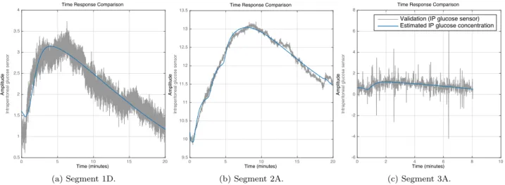
Figure 5: Examples of identification of arterial to peritoneal glucose dynamics, i.e. the transfer function HP(s), for one segment of each animal experiment. The grey signal represents the IP sensor signal, while the blue signal shows the IA sensor signal transferred through HP(s). Beware of the scaling of the vertical axes, and that they have no unit, since the signals are uncalibrated. The seemingly variable signal-to-noise ratio is mostly due to the scaling. Copyright: CC BY-NC-SA 4.0.
Combining Eqs.1and 2gives Eq.3: h−1
S,IP(GIP(s)) HP(s) = h
−1
S,IA(GIA(s)) (3) For each segment of the experiments, the parameters of HP(s) were estimated by minimization of normal-ized root mean square error (NRMSE), using the Sys-tem Identification Toolbox of Matlab R2015a (Math-works, Inc., MA, USA). The resulting values of T and
τ for each experiment segment are reported along with the NRMSE fitness value [%] in Table 1. The “fitness
value” is 1−NRMSE, i.e. 100% corresponds to a
per-fect fit.
2.5.3 Sensor dynamics
In order to identify HP(s), the sensor dynamics had to be compensated. In practice, the sensor dynamics were inverted at both IP and IA sites before the system was identified, resulting in Eq.4based on Eq.3:
GP(s) = HP(s)GB(s) (4) where GP(s) = h−1
S,IP(GIP(s)) and GB(s) = h−1
S,IA(GIA(s)), which requires that the sensor dynamics are invertible. The sensor dynamics are described by the nonlinear differential equation:
d∆L(t)
dt =
1
T0(Keq∆LmaxGloc(t)
−(1 + Keq∆Lmax)Gloc(t))
(5)
where Gloc(t) is the glucose concentration at the sen-sor location (i.e. GB(t) for the IA sensor and GP(t) for the IP sensor), ∆L(t) is the sensor signal (i.e. GIA(t) for the IA sensor and GIP(t) for the IP sensor) re-flecting a length change in the gel caused by the glu-cose concentration in the surrounding fluid, Keq is an equilibrium constant, ∆Lmax is the maximum value
of ∆L(t), and T0 is the characteristic time constant. The values of Keq and ∆Lmax are extracted from the
static parts of the 3-point calibration, i.e. when the signal has stabilized after placing the sensor in each of the 3 solutions. T0 is extracted from a transient sen-sor response, also during the 3-point calibration. The identified parameter sets for all sensors are reported in Table2.
Eq.5 can be solved with respect to Gloc(t) to yield:
Gloc(t) = 1 Keq∆Lmax
∆L(t) + T0d∆L(t)dt 1− ∆L(t)
∆Lmax
(6) Since the sensor dynamics described by Eq. 5 is minimum-phase, it can be inverted, but the inversion amplifies the high-frequent noise due to the differenti-ation of the sensor signal. The original sensor signals and estimated IA and IP glucose concentration for one segment of each experiment are presented in Figure4. The inverted signals are smoothed by zero-phase aver-aging over 5 samples, but only for the illustrations (i.e. not for the input to system identification).
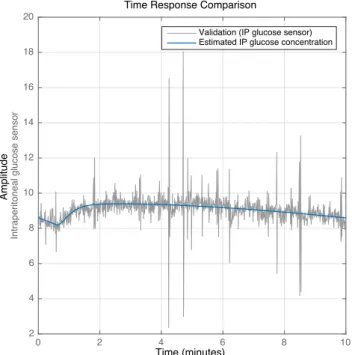
2.5.4 Calculation oftmax/2
For all segments of the trial containing a single glucose bolus, the time to reach half of the maximum IP sensor signal (denotedtmax/2) was calculated. Since the
base-line was unknown, a model of the dynamics from the glucose bolus to the IP glucose sensor signal was identi-fied for each segment in order to find a better estimate
0 5 10 15 20
Intraarterial glucose sensor
5 6 7 8 9 10 11 12 13 14 15
Validation (IA glucose sensor) Estimated IA glucose concentration Time Response Comparison
Time (minutes)
Amplitude
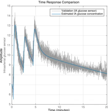
Figure 6: Example of identification of the dynamics HC(s)hS,IA(·) from the glucose bolus to the
arterial glucose concentration for segment 2A. The grey signal represents the IA sensor signal, while the blue signal shows a glucose bolus transferred through HC(s)hS,IA(·).
Be-ware that the vertical axis has no unit, since the signals are uncalibrated. Copyright: CC BY-NC-SA 4.0.
of tmax/2. This corresponds to HC(s)HP(s)hS,IP(·) in
Figure 3. For experiment 1 and 3 the sensor types at the IA and IP locations were identical, so one can use HC(s)hS,IP(·) = HC(s)hS,IA(·), representing the
dy-namics from the glucose bolus to the IA glucose sensor signal. These dynamics were modelled by a time de-lay and a transfer function with 2 zeros and 3 poles, which gave satisfactory fit. The resulting fit values, time delays and tmax/2 are reported in Table 1. For experiment 2, these values are not reported, since only multi-bolus series were included in that experiment.
2.5.5 Protocol adjustments
Table 1: Results summarized. The bottom part shows the median value, mean value and standard deviation for the identified parameters.
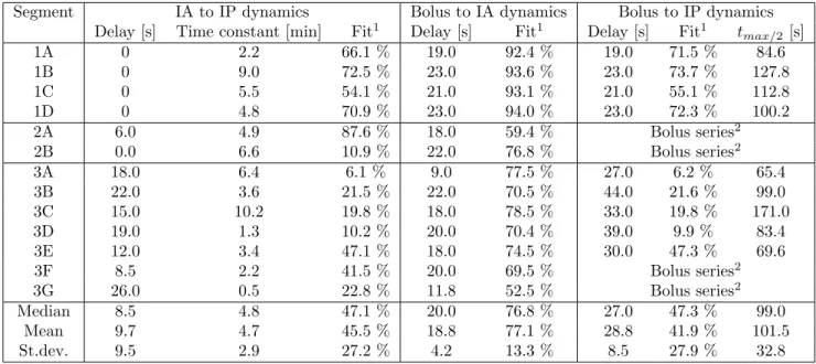
Segment IA to IP dynamics Bolus to IA dynamics Bolus to IP dynamics Delay [s] Time constant [min] Fit1 Delay [s] Fit1 Delay [s] Fit1 tmax/2 [s]
1A 0 2.2 66.1 % 19.0 92.4 % 19.0 71.5 % 84.6
1B 0 9.0 72.5 % 23.0 93.6 % 23.0 73.7 % 127.8
1C 0 5.5 54.1 % 21.0 93.1 % 21.0 55.1 % 112.8
1D 0 4.8 70.9 % 23.0 94.0 % 23.0 72.3 % 100.2
2A 6.0 4.9 87.6 % 18.0 59.4 % Bolus series2
2B 0.0 6.6 10.9 % 22.0 76.8 % Bolus series2
3A 18.0 6.4 6.1 % 9.0 77.5 % 27.0 6.2 % 65.4
3B 22.0 3.6 21.5 % 22.0 70.5 % 44.0 21.6 % 99.0
3C 15.0 10.2 19.8 % 18.0 78.5 % 33.0 19.8 % 171.0
3D 19.0 1.3 10.2 % 20.0 70.4 % 39.0 9.9 % 83.4
3E 12.0 3.4 47.1 % 18.0 74.5 % 30.0 47.3 % 69.6
3F 8.5 2.2 41.5 % 20.0 69.5 % Bolus series2
3G 26.0 0.5 22.8 % 11.8 52.5 % Bolus series2
Median 8.5 4.8 47.1 % 20.0 76.8 % 27.0 47.3 % 99.0
Mean 9.7 4.7 45.5 % 18.8 77.1 % 28.8 41.9 % 101.5
St.dev. 9.5 2.9 27.2 % 4.2 13.3 % 8.5 27.9 % 32.8
1Fit is defined as 1−N RSM E (normalized root mean square error), i.e. 100 % is perfect fit, as described in Section2.
2Segments 2A, 2B, 3F and 3G contained bolus series and have thus no calculation of “Bolus to IP dynamics” ortmax/2.
3 Results
Figure4 shows examples of sensor dynamics inversion and the resulting IA and IP glucose level estimates for segments 1A, 2A and 3E. The relatively large difference between IA sensor signal and IA glucose concentration estimate in experiment 2 demonstrates the slow sensor dynamics of the 3ABP-beta sensors and confirms that the glucose estimates become similar to those enced with the normal 3ABP-alpha sensors in experi-ments 1 and 3. It can also be seen that the IP glucose concentration estimates of experiment 3 were noisier than in the other experiments.
Figure5shows examples of system identification for the IA to IP dynamics, HP(s), for segments 1D, 2A and 3A. These are considered to be representative of the overall experiment. Segment 3A shows that even with a relatively low fit value of 6.1 % (see Table 1), the resulting estimate is reasonable.
Figure6and Figure7show examples of system iden-tification for the dynamics from the glucose bolus to the IA and IP sensor signals, respectively, for segments 2A and 3C. These segments are selected as a good rep-resentation of the overall result.
Table 1summarizes the identified delays, time con-stants and goodness of fit (NRMSE fitness value) for
each segment of the three animal experiments. It shows also the identified dynamics from the glucose bolus in-fusion to the IA and IP sensor signals, and the corre-spondingtmax/2, for the single glucose bolus segments.
The bottom part shows median value, mean value and standard deviation for the identified parameters.
Table2shows sensor parameter sets for all the work-ing IA and IP sensors.
4 Discussion
0 2 4 6 8 10
Intraperitoneal glucose sensor
2 4 6 8 10 12 14 16 18 20
Validation (IP glucose sensor) Estimated IP glucose concentration Time Response Comparison
Time (minutes)
Amplitude
Figure 7: Example of identification of the dynam-ics HC(s)HP(s)hS,IP(·) from the glucose
bo-lus to the peritoneal glucose concentration for segment 3C. The grey signal represents the IA sensor signal, while the blue signal shows a glucose bolus transferred through HC(s)HP(s)hS,IP(·). Beware that the
verti-cal axis has no unit, since the signals are un-calibrated. Copyright: CC BY-NC-SA 4.0.
size. A possible cause of faster dynamics in our trials is that we did not include sensor dynamics in our calcula-tions, since the sensor dynamics are separate from the physiology and should be excluded when characterizing the intrinsic properties of the human body.
The “IA to IP dynamics” system identification pro-cedure performs well. Although the reported fit val-ues are moderate, with a mean fit value of 45.5% (SD 27.2%), it can be seen in Table 1 and the example plot for Segment 3A in Figure5that the low fit values originate mostly from the noisy IP glucose concentra-tion estimates in experiment 3. In order to get sat-isfactory results, a manual optimization of delays and initial time constants was needed; otherwise the algo-rithm terminated at local optima with much lower fit values, as mentioned above. This can be interpreted as a weakness of the algorithms, but it is generally com-mon in system identification to require some manual optimization when local minima are present.
When giving IV glucose boluses it was anticipated that the increase in circulatory glucose would reach the femoral artery (IA sensor) and the capillaries in
the peritoneal lining at approximately the same time. However, that the measured IP glucose level should start to increase more or less concomitant with the glu-cose level in the peritoneal lining was a surprise. This indicates that IP sensors, at least the one in experiment 1, may have been measuring directly in contact with the capillaries in the peritoneal lining, i.e. with just a thin layer (consisting of little more than the capillary wall and the sensor membrane) between blood and the sensor element, leading to a negligible transport delay through IP fluid diffusion or convection.
In the present study, glucose boluses were used. A glucose bolus effectively is an impulse, which is better suited for identification purposes than slower glucose changes. This is because an impulse is richer in its frequency content and thus excites a wider range of dynamic modes in the system. In future experiments, a continuous IV glucose infusion given in a manner to imitate glucose excursions following a meal, may be used. This would document in a more lifelike manner whether or not IP glucose sensing is a realistic alterna-tive in humans when designing an artificial pancreas.
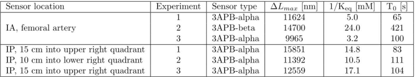
Table 2: Sensor types and parameter sets.
Sensor location Experiment Sensor type ∆Lmax [nm] 1/Keq[mM] T0 [s]
IA, femoral artery
1 3APB-alpha 11624 5.0 65
2 3APB-beta 14700 24.0 421
3 3APB-alpha 9965 3.2 100
IP, 15 cm into upper right quadrant 1 3APB-alpha 15851 14.8 83
IP, 10 cm into lower right quadrant 2 3APB-alpha 11392 10.5 111
IP, 15 cm into upper right quadrant 3 3APB-alpha 12559 17.1 104
a spin-off company from the university the authors are affiliated with, c) they are designed for sensing in body fluids similar to peritoneal fluid, and d) there are no alternative sensors on the market that are designed for IP use.
In all segments, and especially visible in experiment 3, the bolus infusions caused a small negative dip in both IA and IP sensor signals. This is probably a temperature effect; the glucose infusions were at room temperature (20–22◦C) and the sensors are sensitive
to temperature. In future, this artifact may thus be avoided by using glucose boluses at body temperature. Assuming that it affected equally the IA and IP sen-sors, its effect on the identification of HP(s) in the pre-sented study is negligible.
In experiment 2, and thereby in 2 out of the 13 re-ported segments, a slightly different sensor type was used at the IA location. The results do not differ much if only the 11 segments with identical sensor types are included. In other words, it does not affect the conclu-sions of the paper.
Calibration of the IP sensors to peritoneal fluid was not performed. Some IP fluid was sampled and anal-ysed ex vivo before bolus infusions were initiated in experiment 1, and the glucose value of this sample was consistent with the blood sample taken at the same time, but there was not enough IP fluid for more sam-pling without disturbing or possibly harming the sen-sors (e.g. by pushing and squeezing the animal’s ab-dominal region in order to collect fluid) as well as the animal itself and possibly the dynamics to investigate in the experiment. Thus, in general there was a lack of a suitable reference for the IP sensors. They were only carried through a three-point calibration before inser-tion into peritoneum. The amplitudes and offsets of the IP sensor signals of this experiment were manually set. Thus, the absolute accuracy of the sensors cannot be analysed, and only the time response has been re-ported. However, knowledge about this time response is valuable as it demonstrates the intrinsic rapid glu-cose sensing in peritoneum independently of the sensor itself.
These experiments were performed in pigs. Since pigs and humans have different anatomy and
physiol-ogy, one cannot yet conclude about how the IP sensor response will perform in humans. However, we have seen that in pigs, IP sensors may have a substantially faster response than SC sensors – faster than previously reported byBurnett et al.(2014). Even if dynamics are different in humans, one may expect that IP response will be faster than SC response even in humans. Clin-ical trials in humans are needed to confirm this.
Glucose dynamics may differ between different parts of the peritoneum. Peritoneal fluid is believed to be produced in the lower part of peritoneum and absorbed mainly in the upper part close to diaphragma (Patel and Planche,2013), which could explain why our study (and the previous study (Burnett et al., 2014)) shows variable dynamics. Moreover, in the present study we observed negligible time delays both in the lower and upper right quadrant. This result may have two in-terpretations: 1) that the present understanding of the peritoneal fluid only being secreted in the lower peritoneal cavity is questionable, or 2) that a signifi-cant part of the intraperitoneal glucose is secreted di-rectly through the peritoneal lining. It is also unclear whether the IP sensors were actually measuring con-centrations representative for the peritoneal fluid or rather at direct diffusion from capillaries in visceral or parietal peritoneal lining. It is challenging to take sam-ples for reference analysis from any of these sites, and thus there is currently a lack of a proper calibration method.
The sensors used in the IA and IP locations were designed for use in blood/fluids and cannot at present be inserted in the SC space without getting destroyed. Thus, we had to use a different sensor type for the SC location. Accordingly, due to the different sensors used, the SC sensor readings could not be used in sys-tem identification and calculation of tmax/2. In the
present study the SC sensor readings can be considered as an illustration of the qualitative difference between SC and IP glucose dynamics.
In other words, it would be more beneficial to focus on faster insulin analogues and new insulin infusion loca-tions, than to focus on the sensor location. However, we hold that both the insulin absorption dynamics and the sensing dynamics must be improved in order to con-struct a robust artificial pancreas able to normalize or near normalize glucose levels in patients with diabetes. The major value of the present pilot study is that it in-dicates that IP glucose sensing may be nearly as fast as the sensing of glucose levels by beta cells in individuals without diabetes.
5 Conclusions
In spite of variations in the execution of the experi-ments were performed (due to the minor protocol ad-justments described before), the results of these experi-ments are consistent across various sensors, procedures and animals. It is a strong indication of faster glucose dynamics between blood and peritoneum than shown in previous studies and is encouraging for the use of IP glucose sensing in an artificial pancreas, where one of the main open challenges is to achieve sufficiently fast dynamics in the glucose control loop.
6 Acknowledgments
Oddveig Lyng at the Unit of Comparative Medicine, NTNU, and Tine A. Hunt and Sondre Volden of Glu-coSet AS, are acknowledged for their invaluable con-tributions to the animal experiments. Olav Spigset at Dept. of Clinical Pharmacology, St Olavs Hospital, is acknowledged for contribution to the study design.
7 Disclosures
An abstract and a poster with preliminary results from this paper were presented at the ATTD conference in Paris, February 2015. Author N. A. Elvemo is general manager of GlucoSet AS, a company in the glucose-monitoring field. Author R. Ellingsen is board mem-ber of GlucoSet AS. Authors N. A. Elvemo, D. R. Hjelme and R. Ellingsen are shareholders of GlucoSet AS. Author S. M. Carlsen is advisory board member for Prediktor Medical AS, another company in the glucose-monitoring field. All authors except N. A. Elvemo are members of the Artificial Pancreas Trondheim (APT) research group at the Norwegian University of Science and Technology (NTNU), Trondheim, Norway.
References
Bailey, T. S., Chang, A., and Christiansen, M. Clini-cal accuracy of a continuous glucose monitoring sys-tem with an advanced algorithm. Journal of
Dia-betes Science and Technology, 2015. 9(2):209–214.
doi:10.1177/1932296814559746.
Basu, A., Dube, S., Slama, M., Errazuriz, I., Amezcua, J. C., Kudva, Y. C., Peyser, T., Carter, R. E., Co-belli, C., and Basu, R. Time lag of glucose from intravascular to interstitial compartment in humans.
Diabetes, 2013. 62(12):4083–4087.
doi:10.2337/db13-1132.
Boyne, M. S., Silver, D. M., Kaplan, J., and Saudek, C. D. Timing of changes in interstitial and venous blood glucose measured with a continuous subcuta-neous glucose sensor. Diabetes, 2003. 52(11):2790– 2794. doi:10.2337/diabetes.52.11.2790.
Burnett, D., Huyett, L., and Zisser, H. Glucose sens-ing in the peritoneal space offers faster kinetics than sensing in the subcutaneous space. Diabetes, 2014. 63(7):2498–2505. doi:10.2337/db13-1649.
Cengiz, E. and Tamborlane, W. V. A tale of two com-partments: Interstitial versus blood glucose moni-toring. Diabetes Technology & Therapeutics, 2009. 11(s1). doi:10.1089/dia.2009.0002.
Clark, L. C., Noyes, L. K., Spokane, R. B., Su-dan, R., and Miller, M. L. Long-term implantation of voltammetric oxidase-peroxide glucose sensors in the rat peritoneum. Methods in Enzymology, 1988. doi:10.1016/0076-6879(88)37008-4.
Clark, L. C., Spokane, R. B., Sudan, R., and Stroup, T. L. Long-lived implanted silastic drum glucose sen-sors. Transactions - American Society for Artificial
Internal Organs, 1987. 33.
Davey, R. J., Low, C., Jones, T. W., and Fournier, P. A. Contribution of an intrinsic lag of contin-uous glucose monitoring systems to differences in measured and actual glucose concentrations chang-ing at variable rates in vitro. Journal of
Dia-betes Science and Technology, 2010. 4(6):1393–1399.
doi:10.1177/193229681000400614.
Garcia, A., Rack-Gomer, A. L., Bhavaraju, N. C., Hampapuram, H., Kamath, A., Peyser, T., Facchinetti, A., Zecchin, C., Sparacino, G., and Co-belli, C. Dexcom g4ap: an advanced continuous glu-cose monitor for the artificial pancreas. Journal of
Diabetes Science and Technology, 2013. 7(6):1436–
Helton, K. L., Ratner, B. D., and Wisniewski, N. A. Biomechanics of the sensor-tissue inter-face—effects of motion, pressure, and design on sen-sor performance and foreign body response—part ii: Examples and application. Journal of
Dia-betes Science and Technology, 2011. 5(3):647–656.
doi:10.1177/193229681100500318.
Mensh, B. D., Wisniewski, N. A., Neil, B. M., and Bur-nett, D. R. Susceptibility of interstitial continuous glucose monitor performance to sleeping position.
Journal of Diabetes Science and Technology, 2013.
7(4):863–870. doi:10.1177/193229681300700408. Patel, R. and Planche, K. Applied Peritoneal Anatomy.
Clinical Radiology, 2013. 68(5):509–520.
Skjærvold, N. K., Lyng, O., Spigset, O., and Aadahl, P. Pharmacology of intravenous insulin administra-tion: Implications for future closed-loop glycemic control by the intravenous/intravenous route.
Dia-betes Technology & Therapeutics, 2012. 14(1):23–29.
doi:10.1089/dia.2011.0118.
Skjærvold, N. K., ¨Ostling, D., Hjelme, D. R., Spigset, O., Lyng, O., and Aadahl, P. Blood glucose
control using a novel continuous blood glucose monitor and repetitive intravenous insulin boluses: Exploiting natural insulin pulsatility as a prin-ciple for a future artificial pancreas.
Interna-tional Journal of Endocrinology, 2013. 245152:1–8.
doi:10.1155/2013/245152.
Stout, P. J., Racchini, J. R., and Hilgers, M. E. A novel approach to mitigating the physiological lag between blood and interstitial fluid glucose measure-ments. Diabetes Technology & Therapeutics, 2004. 6(5):635–644. doi:10.1089/dia.2004.6.635.
Tierney, S., Falch, B. M. H., Hjelme, D. R., and Stokke, B. T. Determination of glucose levels us-ing a functionalized hydrogel-optical fiber biosensor: Toward continuous monitoring of blood glucose in vivo. Analytical Chemistry, 2009. 81(9):3630–3636. doi:10.1021/ac900019k.