DOI: 10.4301/S1807-17752015000300001
___________________________________________________________________________________________ Manuscript first received/Recebido em: 20/05/2014 Manuscript accepted/Aprovado em: 19/10/2015 Address for correspondence / Endereço para correspondência
H.C.W. Lau, Corresponding author. School of Business, University of Western Sydney, Locked Bag 1797, Penrith, New South Wales 2751, Australia, Tel.: +61 2 96859488, Mobile: +61 459123038. E-mail:[email protected].
Dilupa Nakandala, School of Business, University of Western Sydney, Locked Bag 1797, Penrith, New South Wales 2751, Australia, Tel.: +61 2 96859488, E-mail:[email protected]. Li Zhao, School of Business, University of Western Sydney, Locked Bag 1797, Penrith, New South Wales 2751, Australia, Tel.: +61 2 96859488
Published by/ Publicado por: TECSI FEA USP – 2015 All rights reserved.
DEVELOPMENT OF A HYBRID FUZZY GENETIC ALGORITHM
MODEL FOR SOLVING TRANSPORTATION SCHEDULING
PROBLEM
H.C.W. Lau Dilupa Nakandala Li Zhao
University of Western Sydney, Penrith, New South Wales, Australia
______________________________________________________________________
ABSTRACT
There has been an increasing public demand for passenger rail service in the recent times leading to a strong focus on the need for effective and efficient use of resources and managing the increasing passenger requirements, service reliability and variability
by the railway management. Whilst shortening the passengers’ waiting and travelling
time is important for commuter satisfaction, lowering operational costs is equally important for railway management. Hence, effective and cost optimised train scheduling based on the dynamic passenger demand is one of the main issues for passenger railway management. Although the passenger railway scheduling problem has received attention in operations research in recent years, there is limited literature investigating the adoption of practical approaches that capitalize on the merits of mathematical modeling and search algorithms for effective cost optimization. This paper develops a hybrid fuzzy logic based genetic algorithm model to solve the multi-objective passenger railway scheduling problem aiming to optimize total operational costs at a satisfactory level of customer service. This hybrid approach integrates genetic algorithm with the fuzzy logic approach which uses the fuzzy controller to determine the crossover rate and mutation rate in genetic algorithm approach in the optimization process. The numerical study demonstrates the improvement of the proposed hybrid approach, and the fuzzy genetic algorithm has demonstrated its effectiveness to generate better results than standard genetic algorithm and other traditional heuristic approaches, such as simulated annealing.
Keyword: passenger railway scheduling; fuzzy logic approach; genetic algorithm;
JISTEM, Brazil Vol. 12, No. 3, Sept/Dec., 2015 pp. 505-524 www.jistem.fea.usp.br 1. INTRODUCTION
Passenger railway companies are facing increasing demands nowadays, such as the need for effective and efficient use of resources, the competitive transportation markets, the increasing passenger requirements, the need for service reliability and availability (Fay, 2000). Competing requirements of the efficient use of resources and meeting passenger demands make passenger train scheduling a difficult task. The passenger train schedule planning is important to railway operations due to the fact that the management of passenger train service is mainly based on regular train schedules (Chang, et al., 2000). One of the main issues of passenger train scheduling is the dynamic nature of passenger flows which are uneven in different time-periods of the day (Huang and Niu,2012). How to make suitable train schedule based on the dynamic demand is one of the main problems for railway management. Whilst shortening the passengers’ waiting and travelling time is necessary to improve passenger satisfaction, lowering operational costs is also necessary for railway management. The general problem that passenger railway companies face nowadays is how to maintain a balance between customer service and operational costs, higher operational costs are usually considered to have better customer service level (Chang, et al., 2000). However, no profit making corporation would maximize the total operational costs for perfect service. They would prefer to find an optimum solution which provides an acceptable standard of customer service within limited resources.
Passenger railway scheduling problem has received considerable attention from both practitioners and scholars. However, most of the work is concerned with the use of mathematical programming such as linear programming, which fails to incorporate real-life characteristics and is not easy to apply in real situations. There is limited literature regarding the adoption of a practical approach which capitalizes on the merits of mathematical modeling and heuristics search algorithms to obtain optimized outcomes in an effective way. This paper contributes to the literature by using novel heuristic optimization approaches in the multi-objective passenger railway scheduling problem. Well-developed optimization techniques, standard genetic algorithm (GA) method and hybrid fuzzy GA method, which focus on finding the nearly optimal solutions based on a stochastic search technique are adopted to optimize the total operational costs while maintaining the customer service level based on a list of known constraints. In this research, we proposed a pragmatic approach, taking advantage of readily available and easy to use solutions to put our suggested approach in practice, with specific skills and training. The guidelines and steps we have provided in this paper can be adopted by practitioners to incorporate in solving their scheduling problem with going through complex computation.
The rest of the paper is organized as follows. Section 2 reviews the relevant literature. Section 3 presents the formulation of the model. The standard GA method and fuzzy GA method are proposed in section 3. The application of the fuzzy GA model is illustrated with a numerical study in Section 4, followed by the discussion of the results in section 5. The last section highlights the findings and suggestions for future research.
2. LITERATURE REVIEW
JISTEM, Brazil Vol. 12, No. 3, Sept/Dec., 2015 pp. 505-524 www.jistem.fea.usp.br
train planning and scheduling used a single-objective approach, focusing on either enhancing service level or minimizing operational costs (Chang et al., 2000). Later on, many scholars found the importance of matching customer demand and cost reduction requirements. Multi-objective passenger railway optimization has been under study with results published in various journals. For example, Chang et al. (2000)’s research aims to minimize the operator's total operational costs and minimizing the passenger's total travel time loss. Huisman et al. (2005) argued that not only the timetable itself is important, the reliability of the timetable is even more important. Service to the passengers, efficiency and robustness are three main objectives for passenger railway transportations. Niu (2011) formulated a nonlinear programming model to minimize the overall waiting time and in-vehicle crowding costs. Huang and Niu (2012) formulated an optimized model to maximize passenger satisfaction by shortening the total passenger-time and maximum railway company satisfaction through the lowering of fuel consumption costs.
As railway optimization problem is complicated and it is usually considered as a mix integer linear programming problem, how to find solutions for this problem is widely discussed in the past research. Caprara (2015) classified the railway planning problems to timetabling and assignment problems. He modeled them as mix integer linear programming, and discussed the solution methods and modelling issues. Most of the previous work is concerned with the use of linear programming and other optimization approaches using heuristics and computational intelligence methods. For example, He et al. (2000) developed a fuzzy dispatching model and genetic algorithm to assist the coordination among multi-objective decisions in rail yards dispatching. Vromons and Kroon (2004) described a stochastic timetable optimization model, providing a linear programming model with minimal average delay under certain disruptions. Huisman et al. (2005) gave an overview of operations research models and techniques used in passenger railway transportation, dividing the planning problems into strategic, tactical and operational phases. They pointed out that heuristic approaches are required for short-term railway scheduling problem and real-time control of the passenger railways. Niu (2011) formulated a nonlinear programming model for the skip-station scheduling problem for a congested transit line. Schindl and Zufferey (2015) considered a refueling problem in a railway network and decomposed it in two optimization levels. They proposed a learning tabu search method to solve this problem and the results show good performance of learning tabu search.
JISTEM, Brazil Vol. 12, No. 3, Sept/Dec., 2015 pp. 505-524 www.jistem.fea.usp.br 3. PROPOSED APPROACH
This paper develops a hybrid method for the passenger railway scheduling that minimizes the total operational costs and maintains customer service level for railway companies. Given that the passenger arrival changes during the day and the number of passengers and trains is large, the manual processing methods become impractical for determining the best schedule of the passenger trains.
The following notation is used in the model development. TC = Total operational costs in the objective function
SC =Service cost assigned according to the respective waiting time at stations
VC =Variable cost of operation FC =Fixed cost of operation
C
N =The average number of waiting passengers in station
i C
N =The number of waiting passengers in the ithminute.
di =Number of traveling passengers in the ith minute
i
n =The schedule of train running in the ith minute.
ni=1 means there is a train scheduled in the i
th minute;
ni=0 means there is no train scheduled in the i
th minute.
1
W =Weighting assigned for service costs of fitness function.
2
W =Weighting assigned for variable costs of fitness function.
3
W =Weighting assigned for fixed costs of fitness function.
c
p =crossover rate.
m
p =mutation rate.
g
N =maximum number of generations.
T
M = the maximum frequency of train schedules of a given period.
C
M =the capacity of the respective station.
Total passenger railway operational costs (TC) includes elements such as variable cost (VC), service cost (SC), and fixed cost (FC),
TC=VC+FC+SC (1)
The variable cost (VC) varies at each run of train schedule and includes costs related to human resources, power resources, and maintenance etc.
JISTEM, Brazil Vol. 12, No. 3, Sept/Dec., 2015 pp. 505-524 www.jistem.fea.usp.br
The service cost (SC) is different from the fixed and variable cost and denotes the cost incurred due to the passengers’ waiting time at stations. The longer the waiting time, the higher the service cost. Cost per minute or certain time period is estimated and assigned to each passenger for calculating the final service cost.
The decision variable of our objective function is the schedule of the run of train in each minute niduring the T period. The weighting (Wi) is assigned to each ith element of the objective function for different emphasis. This allows controlling the emphasis on each cost element; customer satisfaction could be given more priority by giving W1 more weight. Thus, the total operational costs are shown as follows:
1 2 3
1
( C* ) ( * ) *
T
i i
TC W N SC W n VC W FC
(2)Constraints of the objective function include the following four aspects:
First, the number of runs of train schedules cannot exceed the limit of the maximum frequency of train schedules of a given period. Thus:
1 T
i T
i
n M
(3)Second, the number of waiting passengers is limited by the available capacity of respective station. Thus:
C C
N M (4)
Third, the weighting of all components must be equal to 1. Thus:
1 2 3 1
WW W (5)
Fourth, the decision variables should be positive integers for runs of scheduled trains
0,1 i
n (6)
3.1. GA method
JISTEM, Brazil Vol. 12, No. 3, Sept/Dec., 2015 pp. 505-524 www.jistem.fea.usp.br START
Parameter setting
Population initialization Objective function
evaluation
G=max generation?
Selection
Crossover
Mutation
The best solution found, output
END
Objective function evaluation Replacement
g=g+1 YES
NO
Fig.1. The standard workflow of GA
Crossover is adopted to exchange information between two parents’ chromosomes for genetic exploration. Not all chromosomes are chosen for crossover. Whether a chromosome is selected or not determined by the crossover ratepc, with a preset value. In the crossover operation, the mating pairs of chromosomes produce two offspring chromosomes. If no crossover happens, the offspring chromosomes are the same as their parents’ chromosomes (Taleizadeh, et al., 2013). In the reproduction process, either one-point crossover or two-point crossover is used (Della Croce et al 1995) and this paper adopts the one-point crossover method.
Mutation is the second genetic operator which provides diversity into future generations so as to prevent them from falling into local optimal. Whether a chromosome is selected, it is determined by the mutation ratepm. A common method is to randomly assign mutation probability values for each gene, and then compare the probability value with the preset mutation rate to determine whether a particular gene will be mutated.
When offspring replace their parent chromosomes, fitness values are calculated for chromosomes in the mating pool. The two least objective function values are replaced with the two best of the new mating pool objective values. The difference between the original solution and the new set provides the degree of improvement of the solution. This process is repeated until the generation counter reaches the pre-set maximum generation value of Ng and the passenger railway schedule is done.
Fig.2 represents the chromosome structure of our study. Each available scheduled train is assigned with binary gene. “1” represents present while “0” represents absence of respective train.
0 0
1
n2 n4
0
n3
0
nT-1
1
nT
n1
JISTEM, Brazil Vol. 12, No. 3, Sept/Dec., 2015 pp. 505-524 www.jistem.fea.usp.br 3.2. Fuzzy GA method
There are possible performance limitations of the standard GA method, such as the overall effectiveness pre-set parameter value that limits the flexibility of the method. If the pre-set parameters, such as crossover rate (pc) and mutation rate (pm) are inappropriate, the fittest solution cannot be found. In standard GA, pcand pm are fixed, which may influence the performance of the algorithm (Peng and Song, 2010). Many scholars suggest improving the standard GA method by changing the pre-set parameters, such as pcand pm(Maiti, 2011). However, as Peng and Song (2010) pointed out, how to change the value of pc and pm in the process is quite complex, as they cannot be defined as precise formula. Fuzzy theory is used in literature to integrate with standard GA to improve the performance of GA (Peng and Song, 2010; Maiti, 2011; Taleizadeh, et al., 2013).
Fuzzy controller for the mutation
rate Fuzzy controller
for the crossover rate
+
++
GA model
+ +
( 1)
c
p t
( )
c
p t
pm( )t
( 1)
m
p t
( )
m
p t
( )
c
p t
( )
a
f t
( 1)
a
f t
( 2)
a
f t
-( 1) d t
Fig.3. The fuzzy GA method
Adapted from Nakandala et al. (2014)
JISTEM, Brazil Vol. 12, No. 3, Sept/Dec., 2015 pp. 505-524 www.jistem.fea.usp.br
of fitness difference of chromosome generation f and the degree of population diversity at generation (t-1), that isd t( 1).
Let f ta( 1) and f ta( 2)be the average fitness values at generation (t-1) and (t-2).
f
is calculated using the following formula (7).
( 1) ( 2)
( 2)
a a
a
f t f t
f
f t
(7)
It is then categorized relatively, and the corresponding fuzzy sets are characterized by its element of fias below and the membership functionf(fi). The fuzzy set off(fi) is shown in Fig.4.
, , , , , , , ,
i
f NLR NL NM NS Z PS PM PL PLR
Where NLR means Negative Larger; NLmeans Negative Large; NMmeans Negative Medium; NSmeans Negative Small; Zis Zero; PSis Positive Small; PMis Positive medium; PL is Positive Large; and PLR is Positive Larger.
NLR NL NM NS Z PS PM PL PLR
f
( )
f fi
1
0
-1.0 -0.8 -0.6 -0.4 -0.2 0 0.2 0.4 0.6 0.8 1.0
Fig.4. The fuzzy set off(fi)
The physical meaning of d is to evaluate the average of bit difference of all pairs of chromosomes in the population and it can be calculated by using the following formula (8):
,
1 1 1
( )
1
( 1)
2
N N M
ik jk
i j i k
g g d
N N M
(8)Where N is the total number of chromosomes in the population, M is the chromosome length,gikis the value of kth gene of ith chromosome, and (gik,gjk) 1 if
ik jk
JISTEM, Brazil Vol. 12, No. 3, Sept/Dec., 2015 pp. 505-524 www.jistem.fea.usp.br
( 1)
d t is categorized by its elements of di and the membership function of d( )di
(shown in Fig.5). Its elements of diare as below:
, , , , , , , ,
i
d VS S SS LM M UM SL L VL
Where VSis Very Small; Sis Small; SSis Slightly Small, LMis Lower Medium; Mis Medium; UM is Upper Medium; SL is Slightly Large; L is Large; and VLis Very Large.
VS S SS LM M UM SL L VL
i d
1
0
0 0.1 0.2 0.3 0.4 0.5 0.6 0.7 0.8 0.9 1.0
( ) d di
Fig.5. The fuzzy set ofd( )di
The two fuzzy controllers determine the change of the crossover rate and mutation rate, that is the values of p tc( )and pm( )t . p tc( )and pm( )t are presented as fuzzy sets in Fig.6 and the Fig. 7.
( ) , , , , , , , ,
c
p t NLR NL NM NS Z PS PM PL PLR
and p tm( )
NLR NL NM NS Z PS PM PL PLR, , , , , , , ,
Where NLR= Negative Larger; NL = Negative Large; NM = Negative Medium; NS = Negative Small; Z = Zero; PS = Positive Small; PM = Positive medium; PL =
JISTEM, Brazil Vol. 12, No. 3, Sept/Dec., 2015 pp. 505-524 www.jistem.fea.usp.br
NLR NL NM NS Z PS PM PL PLR
1
0
-0.1 -0.08 -0.06 -0.04 -0.02 0 0.02 0.04 0.06 0.08 0.1
( )
pc pci
( ) c p t
Fig.6. The fuzzy set ofpc(pci)
NLR NL NM NS Z PS PM PL PLR
1
0
-0.01 -0.008-0.006 -0.004-0.002 0 0.002 0.004 0.006 0.008 0.01
( )
pm pmi
( ) m
p t
Fig.7. The fuzzy set ofpm(pmi)
The main advantage of this hybrid fuzzy GA approach is that it incorporates the experts’ tacit knowledge into the change of the preset parameters p tc( ) and
( ) m
p t
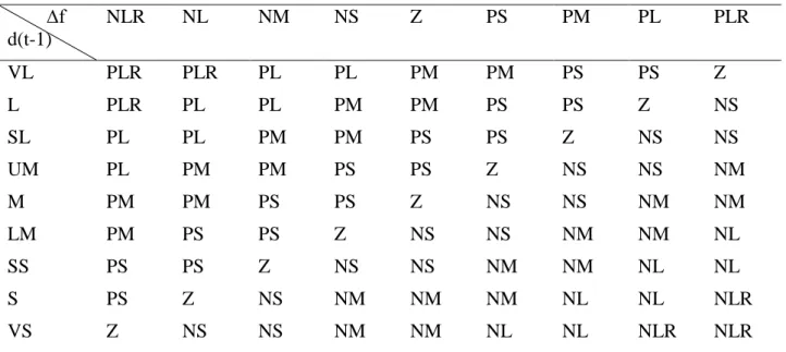
JISTEM, Brazil Vol. 12, No. 3, Sept/Dec., 2015 pp. 505-524 www.jistem.fea.usp.br Table 1. The fuzzy rule table for crossover rate change
∆f d(t-1)
NLR NL NM NS Z PS PM PL PLR
VL PLR PLR PL PL PM PM PS PS Z
L PLR PL PL PM PM PS PS Z NS
SL PL PL PM PM PS PS Z NS NS
UM PL PM PM PS PS Z NS NS NM
M PM PM PS PS Z NS NS NM NM
LM PM PS PS Z NS NS NM NM NL
SS PS PS Z NS NS NM NM NL NL
S PS Z NS NM NM NM NL NL NLR
VS Z NS NS NM NM NL NL NLR NLR
In the fuzzy inference engine, the IF-THEN fuzzy rules are developed based on the expert knowledge and historical data. Table 1 and Table 2 show the rule sets for generating the output of p tc( )andpm( )t . According to the IF-part of the rules, composition result of each rule is calculated, and the results are then put into the implication process to determine the Then-part output fuzzy set with different implication operators. For example, if the degree of fitness difference of chromosome generation f is NLR and the degree of population diversity at generation (t-1) is VL, the crossover rate change would be PLR.
Table 2. The fuzzy rule table for mutation rate change
∆f d(t-1)
NLR NL NM NS Z PS PM PL PLR
VL NLR NLR NL NL NM NM NS NS Z
L NLR NL NL NM NM NS NS Z PS
SL NL NL NM NM NS NS Z PS PS
UM NL NM NM NS NS Z PS PS PM
M NM NM NS NS Z PS PS PM PM
LM NM NS NS Z PS PS PM PM PL
SS NS NS Z PS PS PM PM PL PL
S NS Z PS PS PM PM PL PL PLR
VS Z PS PS PM PM PL PL PLR PLR
JISTEM, Brazil Vol. 12, No. 3, Sept/Dec., 2015 pp. 505-524 www.jistem.fea.usp.br
process of fuzzification. The crisp values of p tc( )and pm( )t are got from the defuzzification stage and used for the adjustment of the crossover rate and mutation rate at generation t.
At generation t, the crossover rate and mutation rate will be adjusted as shown in formula (9) and (10), and GA model will use p tc( )and pm( )t instead ofp tc( 1)and pm(t1) to proceed the search at generation t.
( ) ( 1) ( )
c c c
p t p t p t (9)
( ) ( 1) ( )
m m m
p t p t p t (10)
4. NUMERICAL STUDY
We select one of the busiest stations, named station A, in the railway line, which has a large number of passengers during the morning peak hours. It is assumed that trains are available for one minute time interval, thus at most 20 trains can be run for the given time period 20 minutes to meet demand. Another assumption is that the maximum capacity of the train is 500 passengers.
Table3. First 20 train arrival rate with one minute interval and possible train schedules
Time Demand
(di)
Schedule
(ni)
Waiting passenger
(NCi>=0)
8:00:00 317 n1 317-500*n1
8:01:00 230 n2 NC1+230-500*n2
8:02:00 222 n3 NC2+222-500*n3
8:03:00 178 n4 NC3+178-500*n4
8:04:00 362 n5 NC4+362-500*n5
8:05:00 253 n6 NC5+253-500*n6
8:06:00 287 n7 NC6+287-500*n7
8:07:00 316 n8 NC7+316-500*n8
8:08:00 252 n9 NC8+252-500*n9
8:09:00 217 n10 NC9+217-500*n10
8:10:00 296 n11 NC10+296-500*n11
8:11:00 301 n12 NC11+301-500*n12
8:12:00 340 n13 NC12+340-500*n13
JISTEM, Brazil Vol. 12, No. 3, Sept/Dec., 2015 pp. 505-524 www.jistem.fea.usp.br
8:14:00 234 n15 NC14+234-500*n15
8:15:00 265 n16 NC15+265-500*n16
8:16:00 249 n17 NC16+249-500*n17
8:17:00 215 n18 NC17+215-500*n18
8:18:00 230 n19 NC18+230-500*n19
8:19:00 267 n20 NC19+267-500*n20
The number of passengers waiting equals to the number of passengers who cannot take the train as it is fully occupied or there is no train when they arrive in the station and they need to wait for the next train. By a simple calculation, number of waiting passengers in ith minute (
i
NC ) =number of waiting passengers in (i-1)th minute (NCi1)+number of traveling passengers in i
th minute (
i
d )- travelled passenger in ith minute . Thus:
1 500 * 0
0
i i i i
i
NC d n if NC
NC
otherwise
(11)
The service cost, variable cost and fixed cost coefficient are shown in the following table. Moreover, we assume w1=w2=w3=1/3.
Service cost (Incurred time) : 20
Variable cost (power, staff, and maintenance, etc.) : 10,000
Fixed cost (administration) : 50,000
The Fitness function calculation is shown in formula (12):
TC=1/3*(20* 20 1 i i NC
+10000* 20 1 i i n
+50 000) (12) Subject to: 20 1 20 i i n
(13)0,1 i
n (14)
1000 i
NC (15)
4.1 Simulation runs using the standard GA method
JISTEM, Brazil Vol. 12, No. 3, Sept/Dec., 2015 pp. 505-524 www.jistem.fea.usp.br Table 4. Parameter pre-set values.
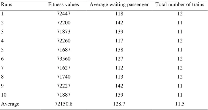
As shown in Table 5, the average fitness value of the 10 simulation runs is 72150.8, with around 129 passengers waiting in each minute and 12 trains running in 20 minutes.
Table 5. Results for 10 simulation runs of standard GA.
Runs Fitness values Average waiting passenger Total number of trains
1 72447 118 12
2 72200 142 11
3 71873 139 11
4 72260 117 12
5 71687 138 11
6 73560 127 12
7 71627 112 12
8 71740 113 12
9 72227 142 11
10 71887 139 11
Average 72150.8 128.7 11.5
4.2 Simulation runs using the hybrid fuzzy GA method
Based on the standard GA method, the values of the input variables of degree of fitness difference (f ) and the degree of population diversity (d) are calculated and the values are 0.00068 and 0.051.
( 1) ( 2) 73740 73690
0.00068
( 2) 73690
a a
a
f t f t
f
f t
(16)
,
1 1 1
( )
1
0.051
( 1)
2
N N M
ik jk
i j i k
g g d
N N M
(17)The membership functions for each variable are:
(1/ 0.2)( 0.2) 0.2 0
( 1/ 0.2)( 0.2) 0 0.2
z
f f
f f
(18)
Parameter Value
Population size 20
Maximum generations 500 Crossover probability 0.80
JISTEM, Brazil Vol. 12, No. 3, Sept/Dec., 2015 pp. 505-524 www.jistem.fea.usp.br
(1/ 0.2)( 0.0) 0 0.2
( 1/ 0.2)( 0.4) 0.2 0.4
PS
f f
f f
(19)
1 0 0.1
( 1/ 0.1)( 0.2) 0.1 0.2
VS
d
d d
(20)
The crisp input values are fuzzified based on the membership functions for each input. The variable f cuts the Z predicate at 0.9966 and PS predicate at 0.0034. Similarly, the variable d cuts the VS predicate at 1. Based on the membership values of the two inputs, four rules are generated from the fuzzy rule blocks (shown in Table 6).
Table 6. Rule generation based on the membership function of f and d.
Rule No “IF” “THEN”
1 The degree of fitness difference IS Zero AND
the degree of population diversity IS very small
Crossover change rate is Negative medium
2 The degree of fitness difference IS positive small
AND
the degree of population diversity IS very small
Crossover change rate is Negative large
3 The degree of fitness difference IS Zero AND the degree of population diversity IS very small
Mutation change rate is positive medium
4 The degree of fitness difference IS positive small
AND
the degree of population diversity IS very small
Mutation change rate is positive large
The composition results are shown in Table 7, Fig. 8 and Fig. 9. Using the most commonly used defuzification method, center of area method, the crisp values of the output variables are calculated. p tc( ) gets a value of -0.04 andpm( )t gets a value of 0.004. Hence the new crossover rate value is 0.76 and the new mutation rate is 0.009 as calculated in formulation (21) and (22).
( ) ( 1) ( ) 0.80 0.04 0.76
c c c
p t p t p t (21)
( ) ( 1) ( ) 0.005 0.004 0.009
m m m
p t p t p t (22)
Table 7. The composition results for the IF part of rules.
Rule No Composition result
Rule 1 0.9966^1=0.9966
Rule 2 0.0034^1=0.0034
Rule 3 0.9966^1=0.9966
JISTEM, Brazil Vol. 12, No. 3, Sept/Dec., 2015 pp. 505-524 www.jistem.fea.usp.br Fig. 8. Implication results of Rule 1 & Rule 2
Fig. 9.Implication results of Rule 3& Rule 4
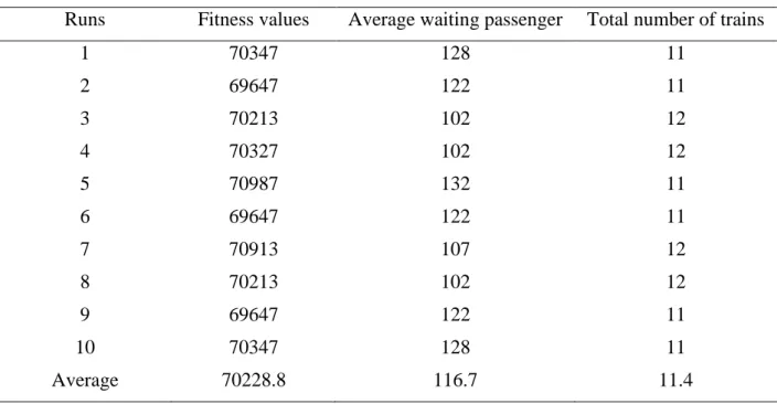
JISTEM, Brazil Vol. 12, No. 3, Sept/Dec., 2015 pp. 505-524 www.jistem.fea.usp.br Table 8. Results for 10 simulation runs of fuzzy GA method.
Runs Fitness values Average waiting passenger Total number of trains
1 70347 128 11
2 69647 122 11
3 70213 102 12
4 70327 102 12
5 70987 132 11
6 69647 122 11
7 70913 107 12
8 70213 102 12
9 69647 122 11
10 70347 128 11
Average 70228.8 116.7 11.4
5. COMPARATIVE RESULTS AND DISCUSSION
Results in section 4 indicate that the hybrid fuzzy GA method runs better results than standard GA method. In order to further evaluate the improvement of the hybrid fuzzy GA method, Simulated Annealing (SA) approach is utilized to compare with the standard GA method and the hybrid fuzzy GA method (Zomaya, 2001). The parameters of SA are given in Table 9.
Table 9. Parameters of SA.
Parameter Value
Initial Temperature 100
Final temperature 0.01
Cooling factor 0.95
Length of Markov Chains 20
JISTEM, Brazil Vol. 12, No. 3, Sept/Dec., 2015 pp. 505-524 www.jistem.fea.usp.br Table 10. Results for 10 simulation runs of SA
Runs Fitness values Average waiting passenger Total number of trains
1 94060 230 14
2 89073 218 13
3 88833 266 11
4 84647 235 11
5 110367 453 10
6 79000 118 14
7 86447 223 12
8 94453 333 10
9 97027 328 11
10 95300 315 11
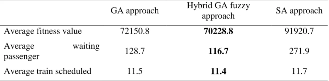
The average fitness value, waiting passenger and number of trains for each method are summarized in Table 11.It can be seen from Table 11 that the performance of standard GA was generally better than the performance of SA, which is partly because of the selection mechanism in GA approach. The selection mechanism of GA approach allows good-quality solutions to be chosen for mating in each generation and crossover operations produce better solutions in each generation. However, there are known limitations of the standard GA methodology, such as the premature convergence which happens because of the fixed control parameters throughout the GA run. These control parameters are chosen based on the experience of users, or some guidelines given in various studies (Lau, Chan and Tsui, 2008; Maiti 2011).
Table 11. Fitness value, waiting passenger and train schedule obtained by different approaches.
GA approach Hybrid GA fuzzy
approach SA approach
Average fitness value 72150.8 70228.8 91920.7
Average waiting
passenger 128.7 116.7 271.9
Average train scheduled 11.5 11.4 11.7
JISTEM, Brazil Vol. 12, No. 3, Sept/Dec., 2015 pp. 505-524 www.jistem.fea.usp.br
of GA, which allows qualitative expression of the control strategies based on experience as well as intuition (Last and Eyal, 2005). Thus, the fuzzy GA approach is proved to have better performance than standard GA and other traditional heuristic approaches, such as SA.
6. CONCLUSION
There has been increasing demand for passenger rail services in recent years. How to effectively use resources to satisfy customers and in the meantime reduce cost is one of the main issues in passenger railway management. Although there are works related to passenger scheduling problem, there is limited literature investigating the adoption of practical approaches that capitalize on the merits of mathematical modeling and search algorithms for effective cost optimization. This study proposed a hybrid optimization model assisting passenger railway managers to solve the multi-objective train scheduling problem, aiming to optimize the total operational cost while maintaining a satisfactory customer service level. The hybrid fuzzy GA model proposed in this study is the seamless integration of the standard GA model and the fuzzy logic approach, both of which are well-developed computational intelligence techniques. The tacit knowledge and expertise of professional is now able to be captured in the fuzzy rules, facilitating the process of finding the optimal schedule. Based on the fuzzy rules and input values, the crossover rate and mutation rate are adjusted to enhance the performance of the search in GA. As illustrated in the numerical study, the hybrid fuzzy GA approach generates better results than both the standard GA method and SA approach in solving passenger railway scheduling problem. Thus, the adoption of the integrated fuzzy GA model is proved to be useful to passenger railway scheduling.
However, due to the complexity of passenger railway transportation, there are limitations in this study which need to be further explored. For example, this research deals with optimizing objectives such as reducing passenger waiting time and operational costs for one station only with time-varying passenger demand. Further research can be done to consider the coordination of a train service along its itinerary by considering the other stops for passenger services, and in turn, passengers' total journey times.
REFERENCE
Caprara, A.(2015). Timetabling and assignment problems in railway planning and integer multicommodity flow. Networks, 66: 1-10.
Chang, YH, Yeh, CH. & Shen, CC. (2000). A multiobjective model for passenger train services planning: application to Taiwain’s high-speed rail line. Transportation Research Part B, 34: 91-106.
Della, Croce, F., Tadei, R. & Volta, G. (1995). A Genetic Algorithm for the Job Shop Problem. Computers & Operations Research, 22: 15-24.
Fay, A. (2000). A fuzzy knowledge-based system for railway traffic control. Engineering application of artificial intelligence, 13: 719-729.
JISTEM, Brazil Vol. 12, No. 3, Sept/Dec., 2015 pp. 505-524 www.jistem.fea.usp.br
Huang, ZP. & Niu, H. (2012). Study on the train operation optimization of passenger dedicated lines based on satisfaction. Discrete dynamics in nature and society, 2012: 1-11.
Huisman, D. & Kroon, LG. (2005). Operations research in passenger railway transportation. Statistica Neerlandica, 49(4):467-497.
Last, M., Eyal, S. (2005). A fuzzy-based lifetime extension of genetic algorithms. Fuzzy sets and systems, 149, 131-147.
Lau, H. C. W., Chan, T. M., Tsui, W. T., Ho, G. T. S. & Choy, K. L. (2009). An Ai Approach for Optimizing Multi-Pallet Loading Operations. Expert Systems with Applications, 36, 4296-4312.
Lau, H.C.W. & Dwight, R.A. (2011). A fuzzy-based decision support model for engineering asset condition monitoring – A case study of examination of water pipelines. Expert Systems with Application, 38 (10), 13342-13350.
Maiti, MK (2011). A fuzzy genetic algorithm with varying population size to solve an inventory model with credit-linked promotional demand in an imprecise planning horizon. European journal of operational research, 213: 96-106.
Niu, HM. (2011).Determination of the skip-station scheduling for a congested transit line by bilevel genetic algorithm. International journal of computational intelligence systems, 6(4): 1158-1167.
Peng, ZH, Song, B. (2010). Research on fault diagnosis method for transformer based on fuzzy genetic algorithm and artificial neural network. Kybernetes, 39(8): 1235-1244.
Schindl, D., Zufferey, N. (2015). A learning tabu search for a truck allocation problem with linear and nonlinear cost components. Naval Research Logistics , 62: 32-45.
Taleizadeh, AA, Niaki, STA, Aryanezhad, MB. & Shafii, N. (2013). A hybrid method of fuzzy simulation and genetic algorithm to optimize constrained inventory control systems with stochastic replenishments and fuzzy demand. Information sciences, 220: 425-441.
Vromans, MJCM. & Kroon, LG. (2004). Stochastic optimization of railway timetables, in: Proceedings TRAIL 8th Annual Congress, Delft University Press, Delft, 423– 445.