Local Renyi entropic profiles of DNA sequences

Open Access

Research article

Local Renyi entropic profiles of DNA sequences

Susana Vinga*

1,2

_{and Jonas S Almeida}

3,4

Address: 1_{Instituto de Engenharia de Sistemas e Computadores: Investigação e Desenvolvimento (INESC-ID), R. Alves Redol 9, 1000-029 Lisboa,} Portugal, 2_{Departamento de Bioestatística e Informática, Faculdade de Ciências Médicas – Universidade Nova de Lisboa (FCM/UNL), Campo dos} Mártires da Pátria 130, 1169-056 Lisboa, Portugal, 3_{Dept Biostatistics and Applied Mathematics, Univ. Texas MDAnderson Cancer Center – unit} 447, 1515 Holcombe Blvd, Houston TX 77030-4009, USA and 4_{Biomathematics Group, Instituto de Tecnologia Química e Biológica –} Universidade Nova de Lisboa (ITQB/UNL), R. Qta. Grande 6, 2780-156 Oeiras, Portugal

Email: Susana Vinga* - [email protected]; Jonas S Almeida - [email protected] * Corresponding author

Abstract

Background: In a recent report the authors presented a new measure of continuous entropy for DNA sequences, which allows the estimation of their randomness level. The definition therein explored was based on the Rényi entropy of probability density estimation (pdf) using the Parzen's window method and applied to Chaos Game Representation/Universal Sequence Maps (CGR/ USM). Subsequent work proposed a fractal pdf kernel as a more exact solution for the iterated map representation. This report extends the concepts of continuous entropy by defining DNA sequence entropic profiles using the new pdf estimations to refine the density estimation of motifs. Results: The new methodology enables two results. On the one hand it shows that the entropic profiles are directly related with the statistical significance of motifs, allowing the study of under and over-representation of segments. On the other hand, by spanning the parameters of the kernel function it is possible to extract important information about the scale of each conserved DNA region. The computational applications, developed in Matlab m-code, the corresponding binary executables and additional material and examples are made publicly available at http://kdbio.inesc-id.pt/~svinga/ep/.

Conclusion: The ability to detect local conservation from a scale-independent representation of symbolic sequences is particularly relevant for biological applications where conserved motifs occur in multiple, overlapping scales, with significant future applications in the recognition of foreign genomic material and inference of motif structures.

Background

Biological sequences are the ultimate support for the description of Biological Systems. In particular, key aspects of sequence analysis are known to play a role in integrated analysis of regulatory networks: for example in motif searching and inference.

Over the last decades and more recently due to the devel-opment of a considerable number of whole genome sequencing projects, several efforts have been made to mathematically model DNA sequences. In particular from the statistical side, the use of Markov based models [1] has widespread and proven to be effective in tackling the problem of data mining of biological sequences, through variable length Markov chains [2,3], interpolated Markov Published: 16 October 2007

BMC Bioinformatics 2007, 8:393 doi:10.1186/1471-2105-8-393

Received: 10 May 2007 Accepted: 16 October 2007

This article is available from: http://www.biomedcentral.com/1471-2105/8/393

© 2007 Vinga and Almeida; licensee BioMed Central Ltd.

models [4], fractal prediction machines [5] for symbolic time series based on Chaos Game Representations [6], to name just a few. Other algorithmic approaches based on the computational side have also proven to be useful [7]. All this effort allowed establishing important relations between the results obtained (computationally and statis-tically) with real biologically significant findings. From these models developed for DNA, it is now apparent that each genome has pervasive [8] motif and compositional characteristics in terms of the frequencies of its constitu-tive L-tuples or L-length motifs, which gave rise to the genomic signature concept [9]. This fact can be directly employed for horizontal transfer detection and character-ization, coding vs. non-coding discrimination [8,10], study and compare DNA through the use of composition profiles [11] and spectra [12] and other applications partly reviewed in [13].

In this regard and more specifically, an important statisti-cal problem in bioinformatics that emerged is the evalua-tion of the number of repetievalua-tions occurring in biological sequences. More generally, they can occur in distinct hier-archical levels, from single symbols [14] to genes. In fact, in a recent paper, the number of gene repetitions was shown to be a key aspect of gene expression and pheno-type [15]. Apparently theses repetitions, not only at nucleotide level, might play a key role in genome organi-zation and functionality of networks. The notions of rep-etitions, entropy and correlation in DNA are unquestionably connected [16-18] and references therein – the degree of predictability of a sequence, which is closely related with its internal repetition and compres-sion, can be measured by its entropy. The major impor-tance of this research has provided evidence that is already too vast to fully account for. In particular, the relation between motif over- or under-representation is usually related with their biological function. This creates the need for an efficient method to analyze, for different parameters sets, the degree or scale of each DNA region.

In a recent report [19], the authors defined a new contin-uous measure of DNA entropy, based on non-parametric density estimation applied to Chaos Game Representa-tion (CGR) and Universal Sequence Maps (USM) within the Rényi theory. The idea therein explored was that there is a close relationship between the statistics of the sequences, given by their constitutive motifs, and their entropy, measured under information theory methodolo-gies. In that report the Rényi entropy was estimated in a global approach, and the measures obtained were com-pared with random sequences by Monte Carlo simula-tion. Although the main concepts were then introduced, that report was incomplete in the sense that just a global analysis was conducted. Specifically, no exploration of local patterns and fine tuned neighboring analysis was

conducted, which is finally allowed by the present work, with the introduction of the concept of the Entropic Profile

(EP).

Entropic profiles were defined previously but in a differ-ent context and scope: they were estimated using the his-tograms of the L-mer or L-tuple frequencies in DNA [20]. In that report the authors could discriminate between ran-dom and natural DNA sequences using the Shannon entropies of the histograms obtained from the CGR for different resolutions or oligomer lengths. Although the same name was used, that previous endeavor focused on a global perspective of sequence entropy [19] whereas this report proposes and investigates a local entropy formula-tion instead. In fact, the results obtained by Oliver and colleagues are global features for each DNA sequence, dif-ferent from the present proposal of local based informa-tion per posiinforma-tion/symbol. Another type of sequence profile also explored was based on linguistic complexity [21] and low entropy DNA zones [22].

In the present report the definition of entropic profile arises from the direct estimation of a local density, derived from the Parzen's window method described before. In our last report this estimation allowed the calculation of a global entropy measure, according to the Rényi defini-tion. This report describes the next logical step of explor-ing complementary methods to access local information as to identify the location and composition of the con-served sequence which existence might have been antici-pated from the global measures of entropy. The rationale is to have a function that assesses, for each position in the sequence (illustrated here for DNA), the information con-tent of L-tuple suffixes directly from the density kernel function estimate. Such a solution should enable the scale-independent extraction of motifs without the need to identify complex state automata for unit succession.

In addition to our preceding report on Rényi entropy for global characterization of sequences, the study reported here also builds on the identification of a kernel function that produces a more accurate density estimation in CGR/ USM projections of symbolic sequences [23]. The more conventional use of symmetrical functions as we did with a Gaussian Parzen kernel produces a rough fit to the char-acteristically fractal nature of iterative map projections. That approximation did suffice for assessment of global entropy [19] but it is not refined enough for the intended density estimation resolved locally at the sequence unit level.

Results and Discussion

This section presents some entropic profiles calculated for the DNA sequences described below. The relation between this values and former results is also investigated. Additionally, the influence of the parameters on the pro-files is discussed.

DNA sequence dataset description

For sake of clarity this report uses the same dataset previ-ously studied [19], thus allowing a comparison of results, in the continuity of the former proposal. In particular, the results for a subset of those sequences with known present motifs will be shown and extensively studied. In order to further test the estimation of the profiles to more chal-lenging datasets, the analysis of whole genomes is also included. More specifically, the detection of Chi sequences in Escherichia coli and Haemophilus influenzae

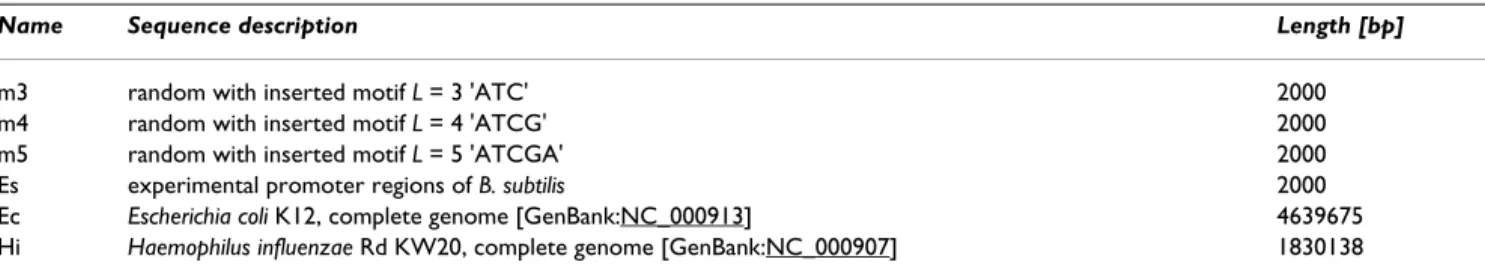
will be assessed. These genomes have been extensively analyzed after the completion of its DNA sequencing projects, thus constituting an excellent dataset to test new procedures. In particular, several important motifs have been studied elsewhere and can be compared directly with the proposed method. The following Table 1 recalls the DNA sequences examined.

All the datasets and additional information are available in the webpage referred to above.

Entropic profiles and parameters optimization

The tests consisted on calculating the entropic profiles (EP) for different combination of parameters L and φand check for particular features. The use of artificial DNA allows the accurate study of the impact of the parameters on the profiles obtained. The results can be directly obtained by using the deduced formulae of Equations 5

for L, φ(xi) and their corresponding normalized values

L, φ(xi) (Eq.3), after specifying the parameters (see

Meth-ods and online software).

The results presented in this section are focused on the analysis of specific positions, known to be important and/ or contain statistical significant motifs as suffixes. For example, Figure 1 represents the profiles obtained for the sequence m4 with the motif 'ATCG' implanted. This motif was implanted n = 20 times at equally spaced positions p = 50+i100, i = 1, ..., 20 (see details in [19]). By studying one of the positions where this suffix ends (as an illustra-tive example p = 353 was chosen), one immediately assesses for which combination of parameters L and φthe maximum values of the profiles is obtained. In this case this maximum is achieved with L = 4 and φapproximately of 1 (one might further search this parameter space con-tinuously in order to optimize φbut this is not pertinent in this explanatory step).

As seen from the Figure 1a) and 1b), there are parameter combinations for which that particular position/suffix is highlighted, with normalized density values way above alternative choices. It was not by chance that the maxi-mum was attained at L = 4, since this is precisely the length of the suffix highly repeated, so L_max ≥ 4 was expected to be a local maximum of EP.

In the other panels of Figure 1 the entropic profile for the complete sequence is plotted, using the parameters previ-ously optimized for the chosen position (p = 353). These plots allow the overview of all the sequence using local information obtained for a specific putative important suffix and, in fact, using this combination of parameters one immediately recovers all the positions where the known motif appears, which are simply the peaks on the graph. Panel d) shows a detail of the EP (from position 300 to 400), clearly illustrating the position where the implanted motif "ATCG" ends, with a density local maxi-mum around EP(353) = 3.9. The expected number of counts under a first-order Markov Chain model would be 10.7 (p-value = 0.0027, z-score = 2.78).

In Figure 1e) and 1f) is also shown the corresponding density estimations on the CGR map for two distinct

ˆ

f

ˆ

g

Table 1: DNA sequence dataset used in this report.

Name Sequence description Length [bp]

m3 random with inserted motif L = 3 'ATC' 2000

m4 random with inserted motif L = 4 'ATCG' 2000

m5 random with inserted motif L = 5 'ATCGA' 2000

Es experimental promoter regions of B. subtilis 2000

Ec Escherichia coli K12, complete genome [GenBank:NC_000913] 4639675 Hi Haemophilus influenzae Rd KW20, complete genome [GenBank:NC_000907] 1830138

The artificial sequences m3, m4 and m5 are obtained by generating random DNA (with symbol emission probabilities pA = pT = pC = pG = 0.25) and

subsequently implanting the motifs described (respectively 'ATC', 'ATCG' and 'ATCGA') in specific positions. The sequence Es corresponds to the concatenation of real DNA from 20 promoter regions of Bacillus subtilis [45, 46], with known consensus structured motif TTGACA-(space)-TATAAT

with at most one point mutation or substitution. The sequences Ec and Hi are the complete genomes of Escherichia coli and Haemophilus influenzae

Entropic profile (EP) for sequence m4

Figure 1

Entropic profile (EP) for sequence m4. Artificial DNA sequence with implanted motif "ATCG" in positions

[50i...53i+100], i = 0, ..., 19 (see Table 1). Several parameter combination L and φare presented, and the corresponding EP val-ues are plotted a) as a function of L for several φand b) as a function of φ(for the same L values). The maximum values of nor-malized estimations g vary along the positions. In this example, position 353 corresponds to the last symbol of one (randomly chosen) occurrence of motif ATCG, and its EP attains a maximum value for L = 4 and φ= 1, with more than 3.5 standard devi-ations from the mean densities (EP _θ(353) = 3.8). c) and d) The complete profile for these parameter values, showing the peaks on the implanted suffix ATCG. The most representative parameter values are plotted. e) and f) The CGR densities obtained from the profiles using the fractal kernel described.

✁ ✂ ✁

✄ ✁ ☎ ✁

✆ ✁ ✝✁

✞ ✟ ✠ ✡ ☛ ☞ ✌ ✍ ✎ ✞✏

✑

✞

✑

✏✒☛

✏

✏✒☛

✞

✞✒☛

✟

✟✒☛

✠

✠✒☛

✓✔✕✖✗✖✔✘✠☛✠

✙

✏✒✞ ✏✒✟☛

✞

✟

✞✏

✚ ✛ ✜ ✢ ✣ ✤✚

✥

✤

✥

✚✦✧

✚

✚✦✧

✤

✤✦✧

✛

✛✦✧

★

★✦✧

✜ ✩✪✫✬✭✬✪✮ ★✧★

I

✛

★

✜

✢

✤✚

✯ ✰✯✯ ✱✯✯✯ ✱✰✯✯ ✲✯✯✯ ✳✴

✳

✲

✳

✱

✯

✱

✲

✴

✵ ✶✷✸✹✺✻✼✽ ✻✹✺✾✼✿ ❀ ❁❂❃

✵❄

I❃ ✱❅

✻✺❆✼✸✼✺✷

❇❈❈ ❇❉❈ ❇❊❈ ❇❋❈ ❇●❈ ❊❈❈ ❍■

❈

■

❉

❇

❊ ❏❑▲▼◆❖P◗ ❖▼◆❘P❙

❚

❘◆▼❯❱❲ ❊❳

I

❲

■❨

❖◆❩P▲P◆❑ ❬❭❪❫

❴

❵

❛

❜❝❞❡

I❝ ❢

❣

❤

✐

❥

❦❧✜♠

I❧ ✤

parameter sets. Comparatively with the Gaussian function this kernel is better adjusted to the CGR square-based geometry and presents a more clear-cut profile, as expected. The darker squares correspond precisely to the implanted motif sub-quadrants.

The following figures present the same results obtained with the other datasets under study.

In Figure 2 the same pattern occurs, with maxima EP(393) = 3.8, obtained for L = 3, again the implanted motif length. It should be mentioned that occasionally, for some positions where the motif "ATC" appears, the

maxima occurs for a value L > 3. This can also happen and simply means that longer, non-implanted motifs appeared more often that would be expected by chance – in this case "ATC" is embedded in a longer significant motif, i.e. is contained in a longer string with potential significance. Interestingly, when plotting all the EP for the sequence using L = 3, one obtains additional, non-implanted motifs, which occurred just by chance – extra peaks with non-equal spacing in Figure 2c) and 2d). In fact, the probability of one specific motif of length 3 (under a null model of symbol equiprobability) is 4-3_, which implies, for a sequence of 2000, that the expected number of counts is roughly equal to 31. This simply

Entropic profile (EP) for sequence m3

Figure 2

Entropic profile (EP) for sequence m3. Artificial DNA sequence with implanted motif "ATC" in positions [30i+1...30i+3], i

= 1, ..., 66 (see Table 1). Same analysis conducted. See legend of Figure 1.

✁ ✂ ✁

✄ ✁ ☎ ✁

✆ ✝ ✞ ✟ ✠ ✡ ☛ ☞ ✌ ✆✍

✎

✆

✎

✍ ✏✠

✍

✍ ✏✠

✆

✆✏✠

✝

✝ ✏✠

✞

✞ ✏✠ ✑✒✓ ✔✕✔✒✖ ✞✌✞

✗

✍ ✏✆ ✍ ✏✝✠

✆

✝

✆✍

✘ ✙ ✚ ✛ ✜ ✢✘

✣

✢

✣

✘ ✤✥

✘

✘ ✤✥

✢

✢✤✥

✙

✙ ✤✥

✦

✦ ✤✥

✚ ✧★✩ ✪✫✪★✬ ✦✭✦

I

✙

✦

✚

✛

✢✘

✮ ✯✮✮ ✰✮✮✮ ✰✯✮✮ ✱✮✮✮

✲

✰

✲

✮ ✳✯

✮

✮ ✳✯

✰

✰✳✯

✱

✱ ✳✯

✴

✴ ✳✯

✵ ✶ ✷✸✹✺ ✻✼✽ ✻✹✺✾✼✿

❀

✾✺ ✹❁❂❃ ✴ ❄

I

❃

✰✮ ❅

✻✺❆✼✸✼✺ ✷

❇❈❈ ❇❉❈ ❇❊❈ ❇❋❈ ❇●❈ ❊❈❈ ❍■

❍

❈ ❏❑

❈

❈ ❏❑

■

■

❏❑

❉

❉ ❏❑

❇

❇ ❏❑

❊ ▲ ▼◆❖P ◗❘❙ ◗❖P❚❘❯

❱

❚P ❖ ❲❳❨ ❇ ❩

I

❨

■

❈ ❬

◗P❭ ❘◆❘P ▼

means that the motif already existed in the random sequence m3 before the implantation took place. The detail graph – Fig. 2d) – shows precisely these "extra" appearances. If one uses a first-order Markov chain model as previously the expected number of counts becomes 60.08 (p-value = 2.8E-10, z-score = 6.2).

A similar interpretation can be made regarding sequence m5: the positions where the suffix "ATCGA" appears have maximal values (x) for L = 5, although with high values in the range L = 4 to L = 7, which indicate nested

signifi-cant motifs. The entropic profile for the complete 2000 base-sequence shows the maxima of the equally spaced motif (see Fig. 3), where it is noticeable an extra peak that corresponds to a previously existing motif ATCGA (end-ing at position 729).

By spanning the parameters space (L, φ) it is possible to

find maximum values for (x). For example, in specific

positions 854 one finds out that attains a maximum

value for memory L = 5 and φ≥ 10 with EP(854) = 7.1, a ˆ

g

ˆ

g

ˆ

g

Entropic profile (EP) for sequence m5

Figure 3

Entropic profile (EP) for sequence m5. Artificial DNA sequence with implanted motif "ATCGA" in positions

[50+100i...54+100i], i = 0, ..., 19 (see Table 1). Position analysis for sequence m5, analogous to those conducted previously. See legend of Figure 1.

✁ ✂ ✁

✄ ✁ ☎ ✁

✆ ✝ ✞ ✟ ✠ ✡ ☛ ☞ ✌ ✆✍

✎

✆

✍

✆

✝

✞

✟

✠

✡

☛ ✏✑✒ ✓✔✓✑ ✕ ☞✠✟

✖

✍ ✗✆ ✍ ✗✝✠

✆

✝

✆✍

✘ ✙ ✚ ✛ ✜ ✢✘

✣

✢

✘

✢

✙

✤

✚

✥

✛

✦

✜ ✧★✩ ✪✫✪★ ✬ ✜✥✚

I

✙

✚

✥

✛

✢✘

✭ ✮✭✭ ✯✭✭✭ ✯✮✭✭ ✰✭✭✭

✱

✰

✱

✯

✭

✯

✰

✲

✳

✮

✴

✵

✶ ✷✸✹✺✻ ✼✽✾ ✼✺✻✿✽❀

❁

✿✻ ✺ ❂❃❄ ✮ ❅

I

❄

✯✭ ❆

✼✻❇ ✽✹✽✻ ✸

❈❉❊ ❋❊❊ ❋❉❊ ●❊❊ ●❉❊ ❍❊❊ ■❏

❊

❏

❑

▲

▼

❉

❈

❋ ◆ ❖P◗❘ ❙❚❯ ❙◗❘❱❚❲

❳

❱❘ ◗❨❩❬ ❉ ❭

I

❬

❏

❊ ❪

high relative value. By using these optima in the EP one obtains a profile that highlights immediately the suffixes where the highly repeated motif appears. Some other maxima appears sometimes (results not shown), but were discovered to correspond to other interpretable extreme values. The expected number of counts for this motif is just 3.07 that, comparing with the observed 21 occur-rences, gives a p-value≈0 (z-score = 10.02).

Finally, Figure 4 shows part of the results for the real DNA sequence in the position corresponding to the ending of the TATA box (motif = "TATAAT"). The graph for this posi-tion shows precisely that L = 6 is an interesting scale to search for. The EP, in contrast to the former ones, does not exhibit a clear trend. In fact, differently to the former sequences, which were artificially generated and pre-sented non-degenerate highly conserved motifs, the real DNA exhibits several point mutations that introduce some "noise" in the estimations. When plotting the com-plete profile for this sequence and observing one detail it is possible to recover the complete structured motif, known to bind to specific transcription factor binding sites, with values EP(TATAAT) = 4.3 and EP(TTGACA) = 3.6. It should be stressed however, that these results are biased towards the sequence itself: in this particular case, the concatenation of the promoter regions of B. subtilis

provided a set with conserved motifs, at least to the point where they could be detected by density estimations. Of course, if non-conservation is allowed up to a higher level, the EP becomes noisier and eventually the signal will be lost, hampering the recovering of any significant motif if no pre-processing correction is performed. The analysis based of Markov chains gives for the TATAAT motif an expected number of counts of 1.60 (p-value≈0, z-score = 10.38) and 0.94 for TTGACA (p-value≈0, z-score = 9.54). The most common motif EP(AAAAAA) = 5.4 is highly periodic which explains the peak, although under a Markov chain it is expected to occur 11.67 (p-value = 0.1245, z-score = 1.15).

The two last datasets are constituted by whole genomes from two Gammaproteobacteria: Escherichia coli K12 and

Haemophilus influenzae Rd (see Table 1 for NCBI GenBank accession numbers).

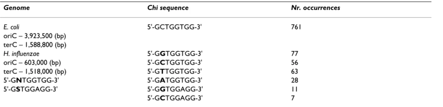
The study of the regions where Chi sequences appear will be analyzed in both genomes. Chi (crossover hotspot instigator) sites are homologous recombinational hotspot octamer sequences which modulate the exonuclease activ-ity of RecBCD. This enzyme is necessary for chromosomal dsDNA repair and integration of exogenous dsDNA, which supports the idea that Chi sites have a biologically functional role [24].

Since Chi motifs are orientation-dependent and strand-specific, the sequence to be analyzed should be previously processed to comply with this property. This means that one should extract the whole genome and use the DNA sequence from the origin of replication up to the terminus plus the reverse complementary sequence, since chromo-some replication in bacteria start from one replication ori-gin (oriC) and proceeds bi-directionally until the replication forks reach the termination site (terC). These pre-processed genomes will conform the 5'->3' direction of replication and therefore will be used throughout the analysis. The oriC and terC positions (referred to the NCBI GenBank database) have been estimated based on experimental data and asymmetric properties [25] and are specified in Table 2.

Chi sequences (see Table 2) are statistically overrepre-sented in the genome of E. coli (5'-GCTGGTGG-3'), appearing more often than would be expected by chance whereas in H. influenzae (5'-GNTGGTGG-3' and 5'-GST-GGAGG-3' show Chi activity) they are known to be less frequent and less conserved. This makes for two different datasets with distinct features that involve a different degree of difficulty to detect these regions.

The study of Chi sites have been subject to many analyses and therefore constitute an excellent test dataset to assess the strength of the entropic profile approach to detect these motifs. In particular several recent papers have assessed its statistical significance using Markov models [1], analyzing the 8-tuple frequency for the whole genome of E. coli [26] and also comparing Chi site conservation in both organisms [24].

The expected number of an 8-tuple in E. coli and H. influ-enzae using a Markov model of order 0 (only nucleotide abundance is taken into account) is respectively 70.796 and 27.926. One immediately sees that in E. coli this motif is highly represented whereas in H. influenzae this fact is less evident.

Interestingly, when analyzing whole genomes, several motifs appear with p-values near 0, i.e. they occur in exceptionally high number when considering a Markov chain model. This fact does not allow their accurate com-parison and is a major drawback of using solely the p-val-ues to assess the statistical significance and correctly compare and order the relative importance of these motifs. Therefore, as explained in the Methods, the nor-malized z-scores are also reported for clarity.

For example, using a first order Markov Chain model the expected number of counts for the chi-sequence in E. coli

corre-sponding z-score of 73.37 and 12.43 respectively puts it in different ranks among all motifs of the same length.

When analyzing one (random) position where Chi sequence ends in E. coli (exactly in the same way as the previous analysis) the following profiles are obtained (Fig. 5). The position p = 35840 shows that the maximum EP values are obtained for parameters (L = 8, φ= 10) and

(L = 9, φ= 5), for which the profiles attain similar values of EP = 8.04 and EP = 8.08 respectively. For L = 7 the motif also appears relevant. The complete profiles for that region are plotted in the panels c) and d), showing strik-ing and evident peaks at the positions where Chi sequences end. The other local maximum corresponds to a chi-related sequence (GCGCTGGC), which in fact shares the 5-mer GCTGG. Indeed, the family containing the

Entropic profile (EP) for sequence Es of the promoter regions in B. subtilis Figure 4

Entropic profile (EP) for sequence Es of the promoter regions in B. subtilis. The peaks in the EP correspond to the structured motif TTGACA-TATAAT. This particular position is well conserved so that the motif is easily detected. Other positions where the motif is degenerated do not exhibit a similar conservation and clear profile. The highest peaks in panel c) correspond to the motif 'AAAAAA', which is repeated more often in the sequence than the previous ones. The overlapping capacity of this motif can partially explain this behavior.

✁ ✂ ✁

✄ ✁ ☎ ✁

✆ ✝ ✞ ✟ ✠ ✡ ☛ ☞ ✌ ✆✍

✎

✆

✎

✍ ✏✠

✍

✍ ✏✠

✆

✆✏✠

✝

✝ ✏✠

✞

✞ ✏✠

✟ ✑✒✓ ✔✕✔✒ ✖ ✝☛✡

✗

✍ ✏✆ ✍ ✏✝✠

✆

✝

✆✍

✘ ✙ ✚ ✛ ✜ ✢✘

✣

✢

✘

✢

✙

✤

✚

✥ ✦✧★ ✩✪✩✧ ✫ ✙✬✛

I

✥

✛

✬

✜

✢✘

✭ ✮✭✭ ✯✭✭✭ ✯✮✭✭ ✰✭✭✭

✱

✰

✱

✯

✭

✯

✰

✲

✳

✮

✴ ✵✶✷✸✹ ✺✻✼ ✺✸✹✽✻✾

✿

✽✹ ✸ ❀❁❂ ✴ ❃

I

❂

✯✭ ❄

✺✹❅ ✻✷✻✹ ✶

❆❇❇ ❆❆❇ ❆❈❇ ❆❉❇ ❆❊❇ ❋❇❇

●

❇ ❍■

❇

❇ ❍■❏

❏

❍■

❆

❆ ❍■

❋

❋ ❍■

❈

❑ ▲▼◆❖ P◗❘ P◆❖❙◗❚❯ ❙❖ ◆❱❲❳❉ ❨

I❳

❏

❇ ❩

P❖❬ ◗▼◗❖▲ ❭❭❪ ❫❴ ❫

trimer CTG, often within the pentamer GCTGG, is very frequent in this genome [27], all with p-values≈0 and highest scoring ranks

When analyzing the genome of H. influenzae and studying one particular position where motif 5'-GGTGGTGG-3' ends (in the example, p = 36532), the following Figure 6 is obtained.

From Figure 6a) is it possible to see that the maximum EP = 0.1252 is obtained for parameters (L = 8, φ= 10), a rel-atively low value when compared with the previous exam-ples so far. Interestingly other peaks exhibit a period of 3 (L = 3 and L = 6) – the motif TGGTGG repeats every 3 and 6 bases and therefore that property is patent in the graph (Figure 6a) through the appearance of this local maxima every 3 bases. When using the above parameters to plot the entire profile one immediately sees that other posi-tions of extremely high significance appear. This is the case of the 8-tuple motifs AAGTGCGG and AGTGCGGT, which corresponds to EP(36549) = 11.1281, p-value≈0, z-score = 174.80, and EP(36550) = 9.7819, p-value≈0, z-score = 186.20, marked in Figure 6d). These motifs appear 867 and 770 times in the genome, which makes them the most common 8-tuples, along with CCGCACTT (820 times; EP = 10.4869, p-value≈0, z-score = 184.47), ACCG-CACT (755 times; EP = 9.5784, p-value≈0, z-score = 210.81) and AAAGTGCG (699 times; EP = 8.8696, p-value≈0, z-score = 97.35), using the same parameters.

As expected, the Chi sites are not detected solely based on EP maximization. In fact, the motif is not especially over-represented when compared with all the others, so it would be impossible to detect based solely on the raw entropic profiles. Furthermore and evident from the fig-ures, the H. influenzae genome has one extremely ubiqui-tous 9-tuple motif, the extensively studied uptake signal sequence (USS+) AAGTGCGGT (appears 740 times) and its inverted complement sequence (USS-) ACCGCACTT (731 times) with a total number of 1471 occurrences.

Their p-values≈0 and their extremely high z-scores of 293.28 and 329.74, puts them in the first rank positions of exceptionality. Furthermore, all the motifs present among the first 25 highest scoring positions greatly over-lap USS sequences [1].

USSs are involved in natural competence, which is a geneti-cally controlled form of horizontal gene transfer in some bacterial species, related to their ability to take up DNA from the surrounding environment (reviewed in [28]). This process allows genetic exchange in bacteria, which is the only organism known to actively take up DNA from the environment and recombine it into their own genome [29]. The DNA uptake machinery on the cell surface pref-erentially binds and takes up fragments containing this specific short sequence. In particular H. influenzae is able to take up double-stranded DNA of its own species and closely relatives, facilitated through the recognition of USS, which are indeed over represented in its genome.

One interesting statistical aspect of the USS distribution, besides its extremely over-representation, is that these sequences appear equally partitioned in both strands and are remarkably and significantly evenly spaced around the chromosome [30]. They can be constituted by the 9 bp core referred to but allowing a longer 29 bp consensus. The USS evolutionary origin and function was recently addressed [31] by confronting two models, preference first hypothesis and a molecular drive hypothesis. Never-theless this issue remains controversial [32].

Through the analysis of H. influenzae complete genome conducted above one obtains peaks on the entropic pro-files precisely at these ubiquitous motifs, which definitely obscures the retrieval of Chi sequences, whose number of occurrences is not at all comparable with USS frequency.

In fact, the profile obtained for the maximum values (L, φ) shows that the Chi sequence (with G) attains a maximum entropic density value of 0.12, which is way below the

Table 2: Description of Chi sites in E. coli and H. influenzae genomes.

Genome Chi sequence Nr. occurrences

E. coli 5'-GCTGGTGG-3' 761

oriC – 3,923,500 (bp) terC – 1,588,800 (bp)

H. influenzae 5'-GGTGGTGG-3' 77

oriC – 603,000 (bp) 5'-GCTGGTGG-3' 56

terC – 1,518,000 (bp) 5'-GTTGGTGG-3' 63

5'-GNTGGTGG-3' 5'-GATGGTGG-3' 28

5'-GSTGGAGG-3' 5'-GGTGGAGG-3' 11

5'-GCTGGAGG-3' 7

The number of occurrences of Chi motifs in the genomes shows that they are overrepresented in E. coli (761 occurrences) but not in H. influenzae

detection level when compared with the value obtained for USS which was equal to EP(AGTGCGGT) = 9.78 and EP(AAGTGCGG) = 11.13. This phenomenon is well understood, and some authors name it "contamination" [1]: the highly overrepresented expressed motif contami-nates the calculation of low expressed segments. The pro-gram R'MES [33] lists precisely USS motifs and their variants showing this behavior. One idea to assess the

sta-tistical significance excluding this bias is to delete, from the original sequence, the regions/positions where this ubiquitous 9-tuple appears [1]. This is approximately comparable to perform exact Markov calculations and therefore can be used to further study the sequence. The obtained values for the transformed sequence were never-theless very low around EP = 0.16 (results not shown). After investigation what might be happening it was found

Entropic profile (EP) for sequence Ec – complete genome of EE. coli Figure 5

Entropic profile (EP) for sequence Ec – complete genome of E. coli. a) and b) Analysis of position 35840 (from the beginning of replication). c) and d) Detail for positions 35800 to 35900. The peaks in the EP correspond to the Chi sequence motif 5'-GCTGGTGG-3'. This particular position is well conserved so the motif is easily detected.

✁ ✂ ✁

✄ ✁ ☎ ✁

✆ ✝ ✞ ✟ ✠ ✡ ☛ ☞ ✌

✍

✆

✎

✆

✝

✞

✟

✠

✡

☛

☞

✌ ✏✑✒ ✓✔✓✑✕ ✞✠☞✟✎

✖

✎ ✗✝✠

✝

✞

✠

✆✎

✎ ✝ ✟ ✡ ☞ ✆✎

✍

✆

✎

✆

✝

✞

✟

✠

✡

☛

☞

✌ ✏✑✒✓✔✓✑ ✕ ✞✠☞✟✎

I

✝

✠

☛

☞

✌

✞ ✗✠☞ ✞ ✗✠☞✝ ✞ ✗✠☞✟ ✞ ✗✠☞✡ ✞ ✗✠☞☞ ✞ ✗✠✌

✘

✆✎✙

✍

✝

✎

✝

✟

✡

☞

✆✎

✚

✑✒✓✔✓✑ ✕

✛

✕✔✜✑

✚

✓✢

✚

✜✑✣✓✤

✥

✣✑ ✜✦ ✖✧☞ ★

I✧ ✆✎ ✩

✠✪ ✍✫ ✬ ✭✫ ✫ ✭✫ ✫ ✍

✞✪ ✫ ✬ ✫ ✬ ✭✫ ✫ ✬

✞ ✗✠☞ ✞ ✗✠☞✝ ✞ ✗✠☞✟ ✞ ✗✠☞✡ ✞ ✗✠☞☞ ✞ ✗✠✌

✘

✆✎✙

✍

✝

✎

✝

✟

✡

☞

✆✎

✚

✑✒ ✓✔✓✑✕

✛

✕✔✜✑

✚

✓✢

✚

✜✑✣✓✤

✥

✣✑ ✜✦ ✖✧✌ ★

I✧✠ ✩

✠✪

that other motifs emerged even when USS were all deleted from the genome.

For example, the 8-tuple AAAATTTT (p-value→1, z-score = -10.70) appears with high EP values, along with other

motifs constituted by long successions of A's and T's. These long adenine-thymine tracts, previously detected for other organisms such as Yeast [34,35], might have an important role due to their strong DNA bending proper-ties [36]. Although the detection of Chi sites failed, other

Entropic profile (EP) for sequence Hi – complete genome of H. influenzae Figure 6

Entropic profile (EP) for sequence Hi – complete genome of H. influenzae. a) and b) Analysis of position 36532 (from the beginning of replication). c) and d) Detail for the EP for positions 36200 to 38200 and 36500 to 36600. The highest peaks in the EP correspond to uptake signal sequences (USS+) 5'-AAGTGCCGGT-3', its reverse complement (USS-) 5'-ACCG-CACTT-3' and related motifs, such as AGTGCGGT and AAGTGCGG. The Chi sites are not particularly well conserved nei-ther overexpressed [24] and nei-therefore are not easily detected with this approach.

✁ ✂ ✁

✄ ✁ ☎ ✁

✆ ✝ ✞ ✟ ✠ ✡ ☛ ☞ ✌ ✆✍

✎

✆

✎

✍ ✏✠

✍

✍ ✏✠

✆ ✑✒✓✔✕✔✒ ✖ ✞✡✠✞✝

✗

✍ ✏✆ ✍ ✏✝✠

✆

✝

✆✍

✘ ✙ ✚ ✛ ✜ ✢✘

✣

✢✤✥

✣

✢

✣

✘ ✤✥

✘

✘ ✤✥

✢ ✦✧★ ✩✪✩✧ ✫ ✬ ✛✥

✬

✙

I

✙

✬

✥

✜

✭

✮ ✯✰✱ ✮ ✯✲ ✮ ✯✲✱ ✮ ✯✳✴ ✵✶✷ ✸✹

✶

✹

✺

✰

✳

✵✶

✵

✹

✻✼✽✾✿✾✼ ❀

❁

❀✿❂✼ ✻✾❃ ✻❂✼❄✾❅❆ ❄✼ ❂❇❈❉ ✳ ❊

I❉ ✵✶ ❋

● ❍■❏ ● ❍■❏❑ ● ❍■❏▲ ● ❍■❏■ ● ❍■❏▼ ● ❍■■ ◆ ❖P◗

❘

❑

P

❑

▲

■

▼

❖P

❖

❑ ❙ ❚❯❱❲ ❳❨❩ ❳❱❲❬❨❭ ❪ ❬❲ ❱ ❫❴❵ ▼ ❛

I

❵

❖P ❜

❳❲❝ ❨❯❨❲❚ ❏❞

❘❡ ❡ ❢ ❣❢ ❤ ❢ ❢ ❣❘ ●❞

❏❞ ❘❢ ❢ ❣❢ ❢ ❣❢ ❢❘

motifs emerged that have notable biological functions and roles in the cell.

This effort highlight an important possible procedure, to be explored further, that one should plot the motifs hier-archically and delete the influence of more ubiquitous motifs that highly "pollute" the calculations, starting from the most exceptional. In fact, from the profile information we could further envisage an algorithm that automatically extracts putative motifs for each position. This is accom-plished by searching the parameters space for which the estimation is maximal for position i:

and then use these parameters to retrieve the suffix .

Using this methodology one obtains precisely the implanted motifs of the previous datasets. As an example, the "TATA"-box referred to before is correctly inferred and also the above mentioned examples with the artificial sequences (Figure 7).

It should be stressed however that this is not the most con-venient procedure for motif inference problems since sev-eral algorithms already exist that perform these searches very efficiently. Nevertheless is interesting to find that combinatorial and probabilistic methodologies are com-parable as the latter come with broader opportunities for theory development albeit leading to advantageous numerical solutions. The observation that there is a close relationship between the overrepresentation, detected by the majority of the algorithms, and the proposed Entropic Profiles with its density and statistical significance meas-ure suggests that it could provide a way of simultaneously finding and statistically classifying the motifs instead of pursuing the two goals separately.

The analysis also showed that the statistical significance z-scores and p-values are unequivocally related with the entropic profiles, since most of the algorithms detected the same motifs. Over-represented motifs exhibit a very low p-value, very near zero, and high z-scores and EP val-ues; common motifs, that appear a median and/or expected number of times, have high p-values and low z-scores, which indicate its non-exceptionality under the Markov chain model considered. These are the motifs that also attain low EP values. The full correspondence between both methods is still under study.

By expressing the density estimation as a function of the suffix counts, one is also allowed to search for

under-rep-resented segments, i.e., those whose density is below aver-age. Although not explored in this work, minimum entropic profile values might also play a role in under-rep-resented motifs detection. In fact, rare motifs/substrings are known to correspond to traits/regions with very spe-cific functions in high precision biological processes. The use of unique sub-strings, or UniMarkers, that appear only once in the genome, recently allowed to locate single nucleotide polymorphisms (SNP's) [37,38]. These unique substrings were shown to be clustered close to genes [39]. All these positions can be detected as low-density areas in the CGR and consequently correspond to local minima in their Entropic Profiles. Another example also related with low-density points is related with 6-tuple palindromes. These short sequences, which often correspond to restric-tion sites, are under-represented in E. coli and in the bac-teriophage lambda [1,40], thus providing a self-protecting effect. More generally this methodology can be used to find heterogeneous traits in the genome, both related with local under- and over- representation of motifs. This result can indicate the presence of foreign material which can have significant applications in the detection of horizon-tal transfer [11].

Conclusion

In this report, Entropic Profiles (EP) were proposed as a novel local information entropy measure for DNA sequences. This function is built on previous work on con-tinuous Rényi quadratic entropy where the Parzen win-dow method was applied to the non-parametric density estimation of the Chaos Game Representation/Universal Sequence Maps (CGR/USM) of a sequence. Subsequently, the estimation was decisively refined to the accuracy that the determination of local entropy requires. This advance, reported elsewhere, introduced a two-parameter fractal-based kernel, instead of Gaussian functions, which is more adequate to the geometry of the CGR domain.

The Entropic Profiles proposed here assess point/symbol normalized deviations from a mean composition signa-ture. EP calculation was based on a density estimation value per position, thus depicting local sequence informa-tion related with the statistical significance of a motif, measured as its global over- or under-representation. Fur-thermore, it was shown that using this kernel the EP can be calculated independently from a particular representa-tion. The local genome scale (or resolution) is defined by the combination of parameters for which a particular suf-fix emerges. Therefore, this scanning procedure identifies simultaneously the position and the scale at with the sequence composition is singular, by focusing and adjust-ing the best parameters locally and then lookadjust-ing back to the overall sequence. There is a strong biological rationale for such an approach as the genome is organized to con-serve motifs at different scales (lengths) and with varying

L _i g x

L L i

max max

, ,

,φ arg max

φ φ

(

)

=

( )

stringency. The underlying hypothesis is that over- or underrepresented motifs may be indicative of important biological functions.

This conclusion was illustrated with the analysis of artifi-cial DNA sequences, reference genomic datasets and also whole genomes from E. coli and H. influenzae, where

known regulatory components and motifs were correctly recovered – both as regards position and scale (length) of the conserved segments. By spanning the parameter space of this new function it was possible to study the local scale for which a given suffix and position were implicit. This effort highlighted the interaction between several meth-odologies in this field. Specifically, it greatly simplifies the

Conserved motif detection and extraction

Figure 7

Conserved motif detection and extraction. By searching the parameter space (L, φ) for a specific position i and finding

the values it is possible to extract the most significant suffix in) the entropic profile

con-text, illustrated here for the first four sequences. Each of the panels corresponds to a different sequence and position where the motif was correctly recovered just by using these maxima: a) m3, b) m4, c) m5 and d) Es (see also Table 1). The profiles for the Lmax and φmax are also shown: apparently one can obtain a non-decreasing function of the positions, which means that

pre-vious suffixes are embedded in the implanted motifs.

✁ ✂ ✁

✄ ✁ ☎ ✁

✆ ✝ ✞

✟✠

✡

☛

☞

✌

✍

✎

✏

✑

✠

✟ ✒✓✔ ✕✓ ✖✗✓ ✘ ☛ ✙✚ ✛✜✢✣✚✣✜

✖

✢ ☛✑ ✠✤

☛✑☛ ✥✦✧ ★✩✪

I✧ ★✩✫✬✭✬✮ ✥☛ ✪

✠

✟ ✫ ✯✧ ★✩

✦✧ ★✩

I✧ ★✩

✰ ✱ ✲ ✳

✴✵

✶

✷

✸

✹

✺

✻

✼

✽

✵

✴ ✾ ✿❀ ❁✿❂❃✿ ❄ ✸ ❅❆ ❇❈❉ ❊❆❊❈

❂

❉ ✷✹✴ ❋✷✹✷ ●❍■ ❏❑▲

I■ ❏❑▼◆❖◆P ●✸ ▲

✵

▼

◗■ ❏❑ ❍■❏❑

I■❏❑

✆ ✝ ✞ ❘ ✆

✟✠

✡

☛

☞

✌

✍

✎

✏

✑

✠

✟ ✒✓✔ ✕✓ ✖✗✓ ✘

✌

✙✚ ✛✜✢✣✚✣✜

✖

✢ ✏

✌

✟

✤

✏

✌

☞ ✥✦■ ❏❑✪

I■ ❏❑✫◆❖◆✮ ✥

✌

✪

✠

✟ ✫ ✯■ ❏❑

✦■ ❏❑

I■ ❏❑

✱ ✰ ✱ ✰ ✰ ✱

✴✵

✶

✷

✸

✹

✺

✻

✼

✽

✵

✴ ✾✿❀ ❁✿ ❂❃✿ ❙ ❉ ❅❆ ❇❈❉ ❊❆❊❈

❂

❉ ✶

✻

✵

❋✶

✻

✺ ●❍■ ❏❑▲

I■ ❏❑▼◆❖◆P ●✺ ▲

✵

✴ ▼ ◗■ ❏❑

❍■❏❑

I■❏❑

L _i g x

L L i

max max

, ,

,φ arg max

φ φ

exploration of fundamental relationships between dis-tinct sequence analysis approaches and concepts such as metrics on strings, information theory and entropy, iter-ated function systems and statistical significance of DNA segments, providing a common ground in kernel-based learning theory.

The procedure proposed here is easily extendable to other kernel function classes, which might be more adequate to model specific traits or genomes. Future work includes the generalization for point mutations and also dealing with nested or embedded motifs.

The proposed entropic profiles provide promising new tools for the study of biological sequences, allowing the quantification of repeatability and identifying key param-eters for which relevant features arise.

Methods

This section recalls the background work that led to the new analysis described here and defines the main con-cepts proposed, namely: the CGR/USM representation of DNA sequences; the assessment of entropy in biological sequences and definition of local Entropic Profile (EP); the use of specialized kernel density estimation functions and its conjugation with the EP method.

CGR/USM representation of DNA sequences and Parzen's method

The CGR/USM representation, introduced in [6] and gen-eralized to higher-order alphabets in [41], allows the mapping of a discrete DNA sequence onto ⺢n_{. Formally,}

the CGR mapping x_i ∈⺢2 _{of a N-length DNA sequence} S = s₁ s₂ ... s_N, s_i ∈ = {A, C, G, T }, i = 1, ..., N is given by Equation 1:

The properties and generalizations of this method have already been studied and extensively applied as a conse-quence to the natural development of alignment-free techniques for sequence comparison [13,42].

As previously, the variables employed in this work will be the USM coordinates sample points {x_i}i = 1, ..., N that

cor-respond to the symbols {s_i}i = 1, ..., N in the original

sequence.

In particular, it was seen in the previous report that these points could be adequately used to estimate the Rényi

entropy of the original sequence through the Parzen's window density estimation method [43]. This is a non-parametric technique used to estimate a probability den-sity function f from a sample. This method is one of the most widely used kernel-based methods and consists on the choice of a weighting function or kernel κ_θ(x). The

estimation (x) of a random vector x is a linear combi-nation of the kernels centered in the observed sample points a_i, i = 1, ..., N, and is defined for a specific window width τ(Eq.2):

In that former report [19] Gaussian or normal distribu-tion funcdistribu-tions were used in order to estimate the Rényi quadratic entropy of the CGR of a given DNA sequence. Due to important algebraic simplifications and properties of the Gaussian kernel it was shown that this calculation was obtained by using a simple potential function of the CGR map.

Entropic profile definition

The former equations provide a natural method to extract local information from a DNA sequence. By calculating

the values θ(xi) for each coordinate xi that represents the

ith symbol in the original sequence and parameter set θ, it is possible to plot, for each position i = 1, ..., N, normal-ized values θ(x) ≡ θ(x; a) of the density function esti-mated previously, obtained as the number of standard deviations from the mean (taking into account all the sample points or symbols, omitted for notation simplifi-cation):

In fact, this corresponds to extracting the local density, estimated for each coordinate that represents a symbol in the original sequence context. For example, if a particular motif appears more often than what would be expected by chance, the density estimation for that particular posi-tion/coordinate will be higher than the average m_θ.

For each parameter set θone can define the Entropic Profile EP_θ(i) ≡ θ(xi), i = 1, ..., N, that measures precisely the

density deviations from the mean in each coordinate, or 

x

x x y x i N y

s

i i i i

i

0

1 1

0 5 0 5 1 2 1 0 0 =

(

)

= +

(

−

)

= =

(

)

− − . , . , ,..., , where if _ii i i i A s C s G s T =

( )

=

( )

=

( )

= ⎧ ⎨ ⎪ ⎪ ⎩ ⎪ ⎪ ⎧ ⎨ ⎪ ⎪ ⎩ ⎪ ’ ’ , ’ ’ , ’ ’ , ’ ’ 0 1 1 0 1 1 if if if ⎪⎪ (1) ˆ f

ˆ _{; ,} ˆ _;

f x a f x a N x a i N i θ

τ κ τ

θ θ

(

)

=

(

)

= ⎛ − ⎝ ⎜ ⎞ ⎠ ⎟ =

∑

1 1 (2) ˆ f ˆ

g gˆ

ˆ ˆ , ˆ ˆ

g x f x m

s m N_i f xi s N f x

N

θ θ θ

θ θ θ θ θ

( )≡ ( )− = ( ) = −

=

∑

with 1 and 1

equivalently, in each last symbol of all the suffixes appear-ing in the original sequence.

Therefore, these values obtained with the kernel estima-tions are related to the statistical significance of the corre-sponding suffix present at that particular position, since they represent a density, which is strongly associated with the degree of repetition of a given suffix in the sequence.

It is worth noting that the proposed entropic profiles are a descriptive measure of local DNA properties and that a full extensive comparison with other methods that search for motifs and assign p-values to the results are out of the scope of this work. Future efforts will quantitatively com-pare these profiles with other models, e.g. Markov chain models, to confirm for the quantitative correspondence between methods on the assessment of under and over-representation of motifs.

Fractal kernel definition

The former approach used Gaussian distribution function to model the generalized Markov models. One possible drawback of this methodology is related with the domain issue above mentioned, since the normal distribution function is defined in ⺢n _{whereas the CGR/USM domain}

is explicitly defined in unit hypercubes. This concern lead to the development of another kernel [23] to be used in the CGR density estimation, which is recalled, reformu-lated and further discussed in this section.

Let χA : X → {0,1}, A ⊂X ⊆⺢, be an indicator or

charac-teristic function such that:

Each function : X → {0,1} with parameters k and x_j

is defined for a point x ∈X as:

where the interval depends on the point x_j ∈X and

on the resolution k chosen:

and N_x

jQ denotes the floor function. The interval above

defined has length V ( ) = 2-k_.

Intuitively, this function rounds the value of x_j, respecting the borders of the regions that represent specific k-tuples,

which are always given by multiples of 2-k _{(see figure 1}

in[19]). This might also be interpreted as the number of common digits of the binary representation of x_j and x, up to the kth _{decimal digit. This is more clearly deduced using}

numeric representation in base 2.

For the CGR mapping ≡ (x(1)_{, x}(2)₎ ∈ _⺢2_{, the 2D step}

function for a point ∈ ⺢2 _{is defined as}

, i.e., the

function is 1 when both coordinates x(1) _{and x}(2) _belong

the above mentioned intervals and is zero otherwise. This is due to the indicator function property χ_A ∩ B = χA χB. For

sake of clarity and notation simplification, in the follow-ing formulas all the variables x and x_j will be assumed in

⺢2 _{otherwise stated, i.e. .}

The kernel κf _{(x) used in this work and extensively}

pre-sented in [23] is based on the linear combination of block functions Ik, using particular resolutions k and a

parame-ter h that defines the height (or weight) of each block:

Additionally, considering the restriction of probability density functions, the following equation is obtained:

since and

.

Defining φas the (constant) ratio between two consecu-tive volumes A_k and A_k-1, k = 1, ..., L (in 2D):

it is possible to express this restriction in terms of φas:

And finally the (normalized) kernel (x) with

parameters L, φand x_j is:

χA x

x A x A

( )

= ∈

∉ ⎧

⎨ ⎩

1 0

if if

I’_{k x, j}

I_{k xj} x _A x

k x j

’ _,

( )

=χ _,

( )

A_{k x, j}

A_{k x, j} =

(

2−k⎢_⎣2kx_j⎥_⎦,2−k_⎣⎢2kx_j⎥_{⎦ +}2−k

)

A_{k x, j} A_{k x, j}

G

x

G

x_j ≡

(

x( )_j1,x( )_j2

)

I_{k x} x x I x I x

k x k x

j _{j j}

,G

(

( )1, ( )2

)

= ’ _,( )1

( )

( )1 × ’ _,( )2

( )

( )2

I_{k x,}G_j

(

x( )1,x( )2

)

≡I_{k x, j}

( )

x

κf κ

L x k k x

k L

x _j x h I _j x

( )

≡

( )

= ⋅

( )

=

∑

, , .

0

κ_{L x k} k k

L

j x x h

,

∫

( )

= ⇒

∑

− =

=

d 1 2 2 1

0

I_{k x, j} x x V A_{k x, j} k

∫

( )

d =

( )

=2−2

V A_{k x} V A V A

k x k x

k

j _{j j}

,G _, ( ) _,( )

( )

= ⎛

⎝

⎜ ⎞ ⎠ ⎟ ⎛

⎝

⎜ ⎞ ⎠ ⎟ = −

1 2 2 2

φ=

( )

φ φ

(

−

)

= − ⇒ = ⋅ − =

( )

⋅

V A V A

h

h h h h

k

k

k

k k k

k

1 1 1 0

1

4 4 4 ,

h k

k L

0 0

1

φ =

=

∑

The underlying idea is to weight, by powers of 4 φ, each step function (x), which corresponds to a sort of

gen-eralized Markov model. An illustration of this kernel func-tion (projected to one-dimensional space) is given in Figure 8 for L = 2 which correspond to three blocks

(x), k = 0,1,2.

Another important property of this function κis its

sym-metry regarding xi and xj, in fact,

since .

Actually, if x_i belongs to the interval A_k means that x_i and

x_j have the same binary expansion up to the k digit, which obviously implies symmetry.

This allows a straightforward generalization under kernel learning theory in which specific transformation of the data with kernel functions induce dot products and norms in other function spaces [44]. In fact, this kernel is related with the Cantor distance in strings, which measures pre-cisely the suffix similarity.

Furthermore, it should be clear that this new fractal kernel is more adjusted to the CGR geometry: instead of Gaus-sian functions that span all ⺢n domain the proposed κ_(x)

is defined on unit hypercubes, which is definitely more in agreement with these iterative maps.

Entropic profiles with fractal kernels

When using the above-defined fractal-based kernel, the expression for the estimation for the entropic profile is significantly simplified, thus allowing its optimal and

κ

φ

φ

φ

L x k k x

k L

k k x k

L

k

k L

j j

j

x h I x

I x

, , ,

,

( )

= ⋅

( )

=

( )

⋅

( )

=

=

=

∑

∑

∑

0

0

0 4

(4)

I_{k x, j}

I_{k x}

j

,

κL, ,φxj

( )

xi =κL, ,φxi

( )

xj Ik x′, i

( )

xj = ′Ik x, j

( )

xi

Example of the proposed fractal kernel κ(x)

Figure 8

Example of the proposed fractal kernel κ(x). Fractal kernel construction projected to one-dimension, for L = 2 and arbi-trary φ.

✁ ✂ ✄

☎ ☎ ✆ ✝ ✞

✟ ✟ ✠ ✡ ☛ ☞ ✌

I

✍

I

✎

✏

✑

✑

I

✒ ✓

✔

✕

✖ ✖ ✗ ✘ ✙

I

N

✚ ✚ ✁ ✂ ✄

☎ ☎ ✆ ✝ ✞

✟ ✟ ✠ ✡ ☛

☞

✎

I

✍

I

✎

✏

✑

✑

I

✒ ✓

✔

✕

✔

✕

✖ ✖ ✗ ✘ ✙

straightforward calculation. In fact, for a particular coordi-nate, each density block is only different from zero if the points in that neighborhood are close, in the sub-quad-rant sense. In other words, for one position, the only non-zero blocks of length k correspond to the nearest points, which are at a distance less than 2-k _apart.

Another important note is that this particular kernel, con-trary to the Gaussian which only has two parameters (mean and variance), depends on the point x_j: in effect, the format of the kernel varies according to the rounding procedure and the particular coordinate x_j considered.

Therefore, the Parzen density estimation for position i or point x_i is given as a function of all the other sample coor-dinates x_j, j = 1, ..., N, and parameter set θ≡ {L, φ}, where L represents the Markov resolution and φis a smoothing parameter:

By simple algebraic simplification and using Eq.4 one obtains a more condensed formula:

Due to the CGR suffix property, the last condition is equivalent of having the same suffix of length k, i.e.,

and if and only if the string

with length k corresponding to the CGR coordinate x_i is the same as the one represented by coordinate xj.

There-fore the sum (x_i) that appears in the last equation

is calculated by simply counting the number of common suffixes of length k shared through all the sequence S_:

where δij is the Kronecker delta and is the suffix of

length k that ends in position i.

Finally, and using this result, the Parzen density estima-tion with this kernel can be simplified to the formula given by the following Equation 5:

Computationally, this is a significant result since it allows

the simplification of L, φ(xi): instead of having to

calcu-late individual kernel function for each point and sum all the contributions, one can simplify the calculation up to a desired resolution or memory length L, greatly reducing the associated algorithmic complexity from quadratic to linear on L and sequence length. In the supplementary MATLAB functions available along this report this simpli-fication was taken into account. In practice this is an important result since low resolutions L are commonly used, remembering that they represent Markov orders. Indeed, most approaches in sequence modeling use Markov orders below 8, which greatly simplifies the calcu-lation time. Some limiting properties of the estimation f

for different φinclude:

These results show that the parameter φis weighting dif-ferent Markov chain models: φ = 0 means that a zero order, background (equal) frequencies are taken, whereas φ→∞ corresponds to weighting higher L-tuples, ignoring the lower order counts, which, in the limiting case, is equivalent to a L-order Markov chain.

In effect, L, φ(xi) can be interpreted as a linear

combina-tion of suffixes counts up to a given memory length, with increasing (φ> 1/4) or decreasing weights (φ< 1/4). These results came up as quite unpredictably, since the kernel defined above was based on a different rationale. It turned out that both perspectives are equivalent in terms of final formulation. It is also noteworthy the relation between this methodology and generalized Markov models and interpolated Markov chains (IMM). In fact, similar pro-files were obtained recently [39] representing the shortest unique substrings in sequences.

ˆ

, , ,

f x

N x

L i L x

j N

i j

φ

( )

= φ

( )

=

∑

1 1 κ ˆ , , f x N I x L i k k L k k L

k x i

j N j φ φ φ

( )

=

( )

( )

= = =

∑

∑

∑

1 4 0 0 1 where

I_{k xj} x_i xi Ak xj xi Ak xj

, ( ) , ( ) , ( ) ( )

( )

= ⎧1 ∈ ∈

0

1 2

1 2

if and

otherwise

⎨⎨ ⎪ ⎩⎪

x_i A

k x_j

( )

,( ) 1

1

∈ x_i A

k x_j

( )

, ( ) 2

2

∈

I_{k x}

j N j , =

∑

1

I_{k x} x count s s c i k i

j N

i s s

j N

i k i

j _ikk_j

, ,

= = − +

∑

( )

=

∑

=

(

)

=

(

[

− +

]

)

1 1

1 1

d s "

s_ik

ˆ , _,

,

f x N

c i k i L L i k k k L k k L φ φ φ

( )

= + = ⋅

(

[

− +

]

)

≥ =

∑

∑

1 1 4 1

1 1 0 (5) ˆ f lim , li ,

φ→∞fLφ

( )

xi = N ⋅c

(

[

i− +L i

]

)

= N ⋅c L

(

i

)

L L

4

1 4 -tuple suffix

m

m ,

φ→0fLφ

( )

xi =1

ˆ