Faculdade de Engenharia da Universidade do Porto
A 2D Stress Analysis of Zirconia Dental Implants: A
Comparison Study
Leonor Gonçalves Piqueiro
P
ROVISIONAL VERSIONThesis submitted to Faculdade de Engenharia da Universidade do Porto as a
requirement to obtain the MSc Degree in Bioengineering
Under the supervision of:
Professor Jorge Américo Oliveira Pinto Belinha
Professor Renato Manuel Natal Jorge
iii
Resumo
Ao longo dos anos, a saúde da boca, bem como o sorriso têm ganho importância, devido ao facto de ser uma das mais importantes capacidades de comunicação de uma pessoa. De facto, a frequência de próteses dentárias removíveis entre os adultos variou entre 13 e 29%, enquanto a frequência das próteses dentárias fixas foi a maior na Suécia (45%) e na Suíça (34%). Ainda assim, os tratamentos de implantes dentários oferecem uma solução que poderá gerar resultados mais satisfatórios para pacientes que não se conseguem adaptar às dentaduras convencionais ou aqueles que já tenham comprometido o osso local.
Existem dois tipos de implantes dentários, que são as próteses dentárias removíveis (RDPs) e as próteses dentárias fixas (FDPs). Os tipos e restauração mencionados possuem nomes diferentes de acordo com a fixação (ou inexistência de fixação) ao osso. As próteses dentárias são aquelas que serão mais aprofundadas neste estudo. Estas próteses são constituídas por três elementos principais, que são a coroa, o abutment e o implante dentário propriamente dito.
A integridade biomecânica dos implantes compreende o comportamento mecânico dos materiais do implante, especialmente, Zircónia. As restaurações de zircónia possuem um papel importante nas FPDs, devido à sua vulnerabilidade mecânica.
Neste trabalho foram usadas técnicas avançadas de discretização numérica – meshless methods – mais especificamente, o Natural Neighbour Radial Point Interpolation Method (NNRPIM) e o Radial Point Interpolation Method (RPIM), mas também, o Método dos Elementos Finitos. O principal objectivo deste trabalho foi compreender o comportamento mecânico dos implantes em zircónia e a resposta do tecido ósseo na presença destes implantes, bem como comparar os três métodos numéricos utilizados neste trabalho, FEM, RPIM e NNRPIM.
Os resultados obtidos mostram que os meshless methods são capazes de produzir campos de deslocamento e tensão mais precisos e suaves quando comparados com malhas de elementos finitos.
v
Abstract
Throughout the years, the health of the mouth and the smile have an increasing importance, due to the fact that is one of the most important interactive communication skills of a person. In fact, the frequency of removable dental prosthesis among adults varied between 13 and 29%, while the frequency of fixed dental prosthesis was the highest in Sweden (45%) and Switzerland (34%). Yet, dental implant treatments offers a solution that may generate more satisfactory outcomes for patients who are not able to adapt to conventional dentures or who have already compromised local host bone.
There are two types of dental implants, which are the removable dental prosthesis (RDPs) and the fixed dental prosthesis (FDPs). The aforementioned types of restorations have different names according to the fixation (or absence of fixation) to the bone. Fixed dental prostheses are the ones that will be mainly focused in this study. These prostheses are constituted by three key elements, which are the crown, the abutment and the dental implant itself. The biomechanical integrity of implants comprises the mechanical behavior of implant materials, especially zirconia. Zirconia restorations have found their indications for FPDs supported by teeth implants due to its mechanical reliability.
It was used advanced discretization numerical techniques – meshless methods – more specifically, the Natural Neighbour Radial Point Interpolation Method (NNRPIM) and the Radial Point Interpolation Method (RPIM), and also the Finite Element Method (FEM)
.The main goal of this work was to understand the mechanical behavior of zirconia implants and the bone tissue response in the presence of such implants and also compare the three numerical methods used in this work, FEM, RPIM and NNRPIM.
The results obtained show that meshless methods are capable to produce more accurate and smooth displacement and stress fields when compared to finite element meshes.
vii
Acknowledgements/Agradecimentos
Em primeiro lugar, gostaria de agradecer ao Professor Jorge Belinha, pelo incansável apoio e por estar sempre disponível ao longo de todo este último semestre. Por todas as dúvidas esclarecidas, por todas as vezes que me ajudo a entender qual o melhor caminho a seguir após cada etapa.
Aos meus amigos Ana Faria, Ana Pereira, José Ribeiro, Madalena Peyroteo e Maria Magalhães por todos os almoços de quarta-feira, mas também por estes 5 anos incríveis que sem vocês não teriam sido a mesma coisa. Aprendi muito com vocês e espero continuar a aprender no futuro. Mas um obrigado especial à Madalena por me aturares 5 meses em Londres. Muito obrigado a todos.
Aos meus amigos do ginásio com quem passei uma boa parte da minha vida, são como uma segunda família para mim, sem dúvida. Por me ouvirem falar, mesmo que não vos interesse nada, por me animarem quando estou mais em baixo e por me terem permitido conquistar tanto. Quer ao nível pessoal, quer a nível técnico. Obrigada.
À Operação Tide 2014, só tenho a dizer ‘Obrigada’. Obrigada por me terem deixado caminhar com vocês, aprender com vocês, viver com vocês, e tantas outras coisas que é difícil descrever por palavras. Muito Obrigada por me fazerem parte deste Caminho.
Ao meu irmão Henrique, por ser sempre o meu melhor amigo em todas as situações. Por me mostrar que vale sempre a pena lutar pelos nossos objetivos e que nada é impossível, basta querer e acreditar em nós mesmo. Obrigada por tudo.
Por fim, aos meus pais, muito obrigada, por me apoiarem sempre, em todas as situações e por acreditarem sempre em mim. Obrigada por me proporcionarem todas as aventuras que vivi até aqui, desde 5 meses em Londres, até uns dia na Colômbia. Obrigada por serem os meus maiores exemplos e por nunca me deixarem de desistir de nenhum sonho. Obrigada por tudo.
ix
Funding
The author truly acknowledge the logistic conditions provided by Ministério da Educação e Ciência– Fundação para a Ciência e a Tecnologia (Portugal), under project funding UID/EMS/50022/2013 (funding provided by the inter-institutional projects from LAETA) and project NORTE-01-0145-FEDER-000022 - SciTech - Science and Technology for Competitive and Sustainable Industries, cofinanced by Programa Operacional Regional do Norte (NORTE2020), through Fundo Europeu de Desenvolvimento Regional (FEDER).
Additionally, the author truly acknowledge the work conditions provided by the department of Mechanical Engineering from FEUP and INEGI.
xi
Índice
Chapter 1 ... 1
Introduction ... 1
1.1 Meshless Methods ... 1
1.1.1. Radial Point Interpolation Method ... 3
1.1.2. Natural Neighbour Radial Point Interpolation Method ... 4
1.2 Objectives ... 5
1.3 Document Structure ... 5
Chapter 2 ... 6
Meshless Methods ... 6
2.1 General Meshless Method Procedure ... 6
2.2 RPIM Formulation ... 7
2.2.1. Influence-domains and nodal connectivity ... 7
2.2.2. Numerical Integration ... 8
2.3 NNRPIM Formulation ... 11
2.3.1. Natural Neighbours ... 11
2.3.2. Influence-Cells and Nodal Connectivity ... 13
2.3.3. Numerical Integration ... 13
2.4 Shape Functions ... 16
Chapter 3 ... 19
Solid Mechanics Fundamentals ... 19
3.1 Stress Components ... 19
3.2 Equilibrium equations ... 20
3.3 Components of strain ... 20
3.4 Constitutive equations ... 22
3.5 Strong form and weak form formulation ... 23
3.5.1. Galerkin weak form ... 23
3.6 Discrete System Equations ... 25
Chapter 4 ... 27
FEMAS ... 27 4.1 FEMAS ... 27Chapter 5 ... 30
Dental Implants ... 30 5.1. Types of Implants ... 30 5.2. Implants Description ... 315.3. Used Materials for Implants ... 32
5.3.1. Zirconia ... 33 5.3.2. Bone ... 34
Chapter 6 ... 36
Numerical Examples ... 36 6.1. The work ... 37Chapter 7 ... 45
Appendix 1 ... 51
Appendix 2 ... 57
Appendix 3 ... 78
xiii
List of figures
Figure 2.1 a.Problem domain with the essential and natural boundaries applied. b.Regular nodal discretization. c.Irregular nodal discretization3 ... 6
Figure 2.2 Influence-domains with different sizes and shapes3 ... 8
Figure 2.3 a.Fitted Gaussian background mesh. b.General Gaussian integration mesh.3 ... 9
Figure 2.4 a.Initial grid-cell. b.Isoparametric square with integration points. c.Initial
quadrature cell with integration points3 ... 9
Figure 2.5 a.Initial nodal set. b.First trial plane. c.Second trial plane. d.Provisional
Voronoï cell. e.Voronoï cell from node n0. f.Voronoï diagram.3 ... 12
Figure 2.6 a.First degree influence-cell. b.Second degree influence-cell.3 ... 13
Figure 2.7 a.Voronoï cell and respective intersection points (PIi). b.Middle points (MIi) and
the respective generated quadrilaterals. c.Quadilateral3 ... 14
Figure 2.8 a.Voronoï cell and respective intersection points (PIi). b.Middle points (MIi) and
the respective generated quadrilaterals. c.Quadilateral3 ... 14
Figure 2.9 Triangular and quadrilateral shapes and the respective integration points.3 ... 15
Figure 2.10 Division in quadrilaterals of the sub-cells3 ... 15
Figure 2.11 Triangular and rectangular shape and respective integration points, xI, using
the Gauss-Legendre integration scheme.3 ... 16
Figure 3.1 Linear deformation of a virtual body3 ... 21
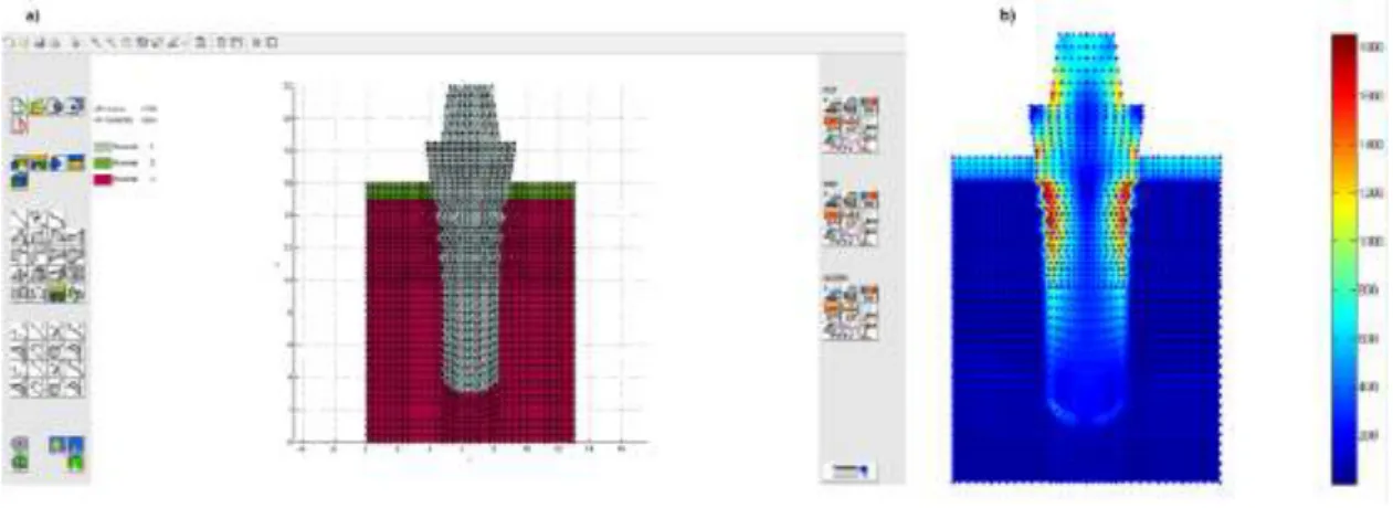
Figure 4.1 FEMAS initial presentation ... 27 Figure 4.2 a.2D Model of a dental implant built in FEMAS b.Stress field of dental implant
obtained in FEMAS... 28 Figure 5.1 Constitution of an Implant ... 31 Figure 6.1 a)3D model of the zirconia implant. b)2D view showing the minimum geometric
dimensions. c)2D view showing the maximum geometric dimensions. ... 37 Figure 6.2 a)3D model of the zirconia implant inserted in the bone block. b)2D section cut
capturing the minimum geometric dimensions. c)2D section cut capturing the
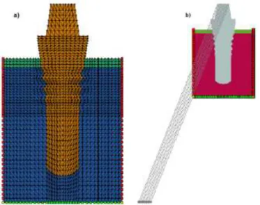
maximum geometric dimensions. ... 38 Figure 6.3 a.Model 1. b.Model 2 ... 38 Figure 6.4 a.Model with essential boundary conditions b.Model with essential boundary
conditions and applied load at 70º ... 39 Figure 6.5 Stress map from type of bone 1, ‘Model 1’, angle 10º, analysed with FEM ... 40 Figure 6.6 Model of a dental implant with the two lines selected ... 41
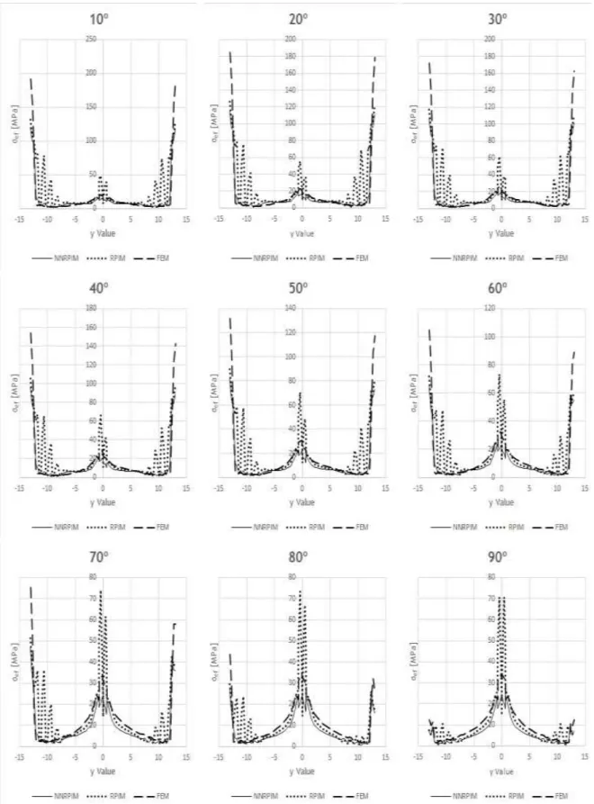
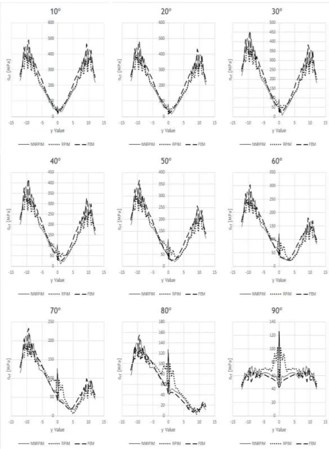
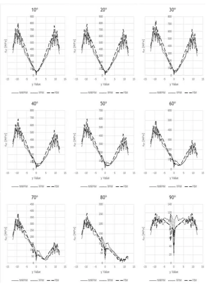
Figure 6.7 a.Stress distribution from bone side, from ‘Model 1’, for an angle of 10º
b.Stress distribution from implant side, from ‘Model 1’, for an angle of 10º ... 41
Figure 6.8 Points of interest in the model of the dental implant ... 42
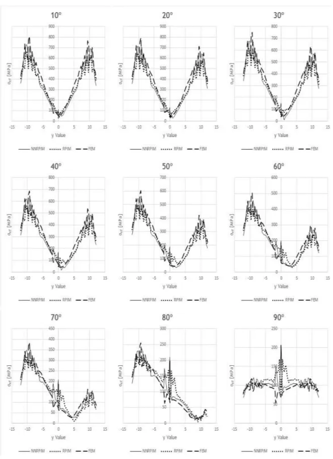
Figure 6.9 Discrete Stress Values for type of bone 4, 'Model 1' and from implant side (point 16) ... 43
Figure A.1 Stress Map from 'Model 1' and bone type 1 ... 52
Figure A.2 Stress Map from 'Model 1' and bone type 2 ... 52
Figure A.3 Stress Map from 'Model 1' and bone type 3 ... 53
Figure A.4 Stress Map from 'Model 1' and bone type 4 ... 53
Figure A.5 Stress Map from 'Model 1' and bone type 5 ... 54
Figure A.6 Stress Map from 'Model 2' and bone type 1 ... 54
Figure A.7 Stress Map from 'Model 2' and bone type 2 ... 55
Figure A.8 Stress Map from 'Model 2' and bone type 3 ... 55
Figure A.9 Stress Map from 'Model 2' and bone type 4 ... 56
Figure A.10 Stress Map from 'Model 2' and bone type 5 ... 56
Figure A.11 Stress distribution from bone side, from ‘Model 1’, from bone type 1 ... 58
Figure A.12 Stress distribution from bone side, from ‘Model 1’, from bone type 2 ... 59
Figure A.13 Stress distribution from bone side, from ‘Model 1’, from bone type 3 ... 60
Figure A.14 Stress distribution from bone side, from ‘Model 1’, from bone type 4 ... 61
Figure A.15 Stress distribution from bone side, from ‘Model 1’, from bone type 5 ... 62
Figure A.16 Stress distribution from bone side, from ‘Model 2’, from bone type 1 ... 63
Figure A.17 Stress distribution from bone side, from ‘Model 2’, from bone type 2 ... 64
Figure A.18 Stress distribution from bone side, from ‘Model 2’, from bone type 3 ... 65
Figure A.19 Stress distribution from bone side, from ‘Model 2’, from bone type 4 ... 66
Figure A.20 Stress distribution from bone side, from ‘Model 2’, from bone type 5 ... 67
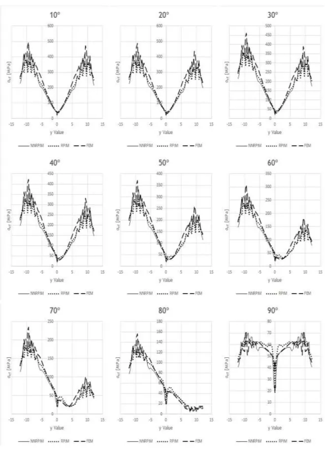
Figure A.21 Stress distribution from implant side, from ‘Model 1’, from bone type 1 ... 68
Figure A.22 Stress distribution from implant side, from ‘Model 1’, from bone type 2 ... 69
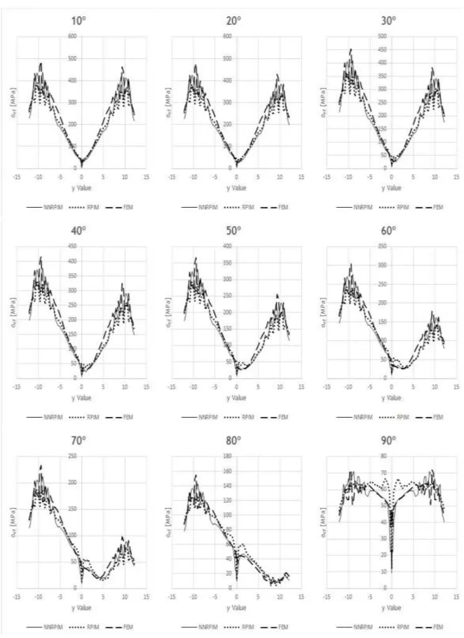
Figure A.23 Stress distribution from implant side, from ‘Model 1’, from bone type 3 ... 70
Figure A.24 Stress distribution from implant side, from ‘Model 1’, from bone type 4 ... 71
Figure A.25 Stress distribution from implant side, from ‘Model 1’, from bone type 5 ... 72
xv
Figure A.27 Stress distribution from implant side, from ‘Model 2’, from bone type 2 ... 74
Figure A.28 Stress distribution from implant side, from ‘Model 2’, from bone type 3 ... 75
Figure A.29 Stress distribution from implant side, from ‘Model 2’, from bone type 4 ... 76
Figure A.30 Stress distribution from implant side, from ‘Model 2’, from bone type 5 ... 77
Figure A.31 Discrete stress values for type of bone 1, 'Model 1' and from bone side ... 103
Figure A.32 Discrete stress values for type of bone 1, for ‘Model 1’ and from implant side .. 104
Figure A.33 Discrete stress values for type of bone 1, 'Model 2' and from bone side ... 105
Figure A.34 Discrete stress values for type of bone 1, for ‘Model 2’ and from implant side .. 106
Figure A.35 Discrete stress values for type of bone 2, 'Model 1' and from bone side ... 107
Figure A.36 Discrete stress values for type of bone 2, 'Model 1' and from implant side ... 108
Figure A.37 Discrete stress values for type of bone 2, 'Model 2' and from bone side ... 109
Figure A.38 Discrete stress values for type of bone 2, 'Model 2' and from implant side ... 110
Figure A.39 Discrete stress values for type of bone 3, 'Model 1' and from bone side ... 111
Figure A.40 Discrete stress values for type of bone 3, 'Model 1' and from implant side ... 112
Figure A.41 Discrete stress values for type of bone 3, 'Model 2' and from bone side ... 113
Figure A.42 Discrete stress values for type of bone 3, 'Model 2' and from implant side ... 114
Figure A.43 Discrete stress values for type of bone 4, 'Model 1' and from bone side ... 115
Figure A.44 Discrete stress values for type of bone 4, 'Model 1' and from implant side ... 116
Figure A.45 Discrete stress values for type of bone 4, 'Model 2' and from bone side ... 117
Figure A.46 Discrete stress values for type of bone 4, 'Model 2' and from implant side ... 118
Figure A.47 Discrete stress values for type of bone 5, 'Model 1' and from bone side ... 119
Figure A.48 Discrete stress values for type of bone 5, 'Model 1' and from implant side ... 120
Figure A.49 Discrete stress values for type of bone 5, 'Model 2' and from bone side ... 121
List of tables
Table 2.1 Integration points coordinates and weights for quadrilateral ‘cells’. ... 10
Table 2.2 Integration points coordinates and weights for triangular ‘cells’. ... 10
Table 5.1 Mechanical Properties of bone cases ... 35
Table A.1 Stress Values for specific points, for type of bone 1 at 10º ... 79
Table A.2 Stress Values for specific points, for type of bone 1 at 20º ... 79
Table A.3 Stress Values for specific points, for type of bone 1 at 30º ... 80
Table A.4 Stress Values for specific points, for type of bone 1 at40º ... 80
Table A.5 Stress Values for specific points, for type of bone 1 at 50º ... 81
Table A.6 Stress Values for specific points, for type of bone 1 at 60º ... 81
Table A.7 Stress Values for specific points, for type of bone 1 at 70º ... 82
Table A.8 Stress Values for specific points, for type of bone 1 at 80º ... 82
Table A.9 Stress Values for specific points, for type of bone 1 at 90º ... 83
Table A.10 Stress Values for specific points, for type of bone 2 at 10º ... 83
Table A.11 Stress Values for specific points, for type of bone 2 at 20º ... 84
Table A.12 Stress Values for specific points, for type of bone 2 at 30º ... 84
Table A.13 Stress Values for specific points, for type of bone 2 at 40º ... 85
Table A.14 Stress Values for specific points, for type of bone 2 at 50º ... 85
Table A.15 Stress Values for specific points, for type of bone 2 at 60º ... 86
Table A.16 Stress Values for specific points, for type of bone 2 at 70º ... 86
Table A.17 Stress Values for specific points, for type of bone 2 at 80º ... 87
Table A.18 Stress Values for specific points, for type of bone 2 at 90º ... 87
Table A.19 Stress Values for specific points, for type of bone 3 at 10º ... 88
Table A.20 Stress Values for specific points, for type of bone 3 at 20º ... 88
Table A.21 Stress Values for specific points, for type of bone 3 at 30º ... 89
Table A.22 Stress Values for specific points, for type of bone 3 at 40º ... 89
xvii
Table A.24 Stress Values for specific points, for type of bone 3 at 60º ... 90
Table A. 25 Stress Values for specific points, for type of bone 3 at 70º ... 91
Table A.26 Stress Values for specific points, for type of bone 3 at 80º ... 91
Table A.27 Stress Values for specific points, for type of bone 3 at 90º ... 92
Table A.28 Stress Values for specific points, for type of bone 4 at 10º ... 92
Table A.29 Stress Values for specific points, for type of bone 4 at 20º ... 93
Table A.30 Stress Values for specific points, for type of bone 4 at 30º ... 93
Table A.31 Stress Values for specific points, for type of bone 4 at 40º ... 94
Table A.32 Stress Values for specific points, for type of bone 4 at 50º ... 94
Table A.33 Stress Values for specific points, for type of bone 4 at 60º ... 95
Table A.34 Stress Values for specific points, for type of bone 4 at 70º ... 95
Table A.35 Stress Values for specific points, for type of bone 4 at 80º ... 96
Table A.36 Stress Values for specific points, for type of bone 4 at 90º ... 96
Table A.37 Stress Values for specific points, for type of bone 5 at 10º ... 97
Table A.38 Stress Values for specific points, for type of bone 5 at 20º ... 97
Table A.39 Stress Values for specific points, for type of bone 5 at 30º ... 98
Table A.40 Stress Values for specific points, for type of bone 5 at 40º ... 98
Table A.41 Stress Values for specific points, for type of bone 5 at 50º ... 99
Table A.42 Stress Values for specific points, for type of bone 5 at 60º ... 99
Table A.43 Stress Values for specific points, for type of bone 5 at 70º ... 100
Table A.44 Stress Values for specific points, for type of bone 5 at 80º ... 100
Abbreviations
DEM Diffuse Element Method EFGM Element-Free Galerkin Method FEM Finite Element Method
GUI Graphical User Interface MFEM Meshless Finite Element Method MLPG Meshless Local Petrov-Galerkin MLS Moving Least Square
NEM Natural Element Method
NNFEM Natural Neighbour Finite Element Method
NNRPIM Natural Neighbour Radial Point Interpolation Method PIM Point Interpolation Method
RBF Radial Basis Functions
RKPM Reproducing Kernel Particle Method RPIM Radial Point Interpolation Method SED Strain Energy Density
Chapter 1
Introduction
Throughout the years, the importance of the health of the mouth and smile have increased, being one of the most important interactive communication skills of a person. Patients and consumers, now demand, not only a healthy mouth, but also a perfect smile. However, the main purpose of dental restorations is to replace missing teeth and, in addition, restore teeth that have been hardly damaged or, for any reason, are not aesthetic, either because of colour, form or contour.1 In order to determine if a single missing tooth can be replaced, it is necessary
in the first instance, to analyse if the tooth in question can be restored or not.2
1.1 Meshless Methods
There is a vast quantity of numerical methods, and they can be defined and classified by three fundamental modules: the field approximation (or interpolation) function, the used formulation and the integration.3 From this point of view, it is possible to define the Finite
Element Method (FEM) and the Meshless Methods as numerical methods.
The Finite Element Method was firstly developed to solve structural problems in the aerospace industry, in the early 1960s and, ever since, has been extended to solve a wide range of problems, from heat transfer to electromagnetics.4
The Finite Element Method is a very recognized and optimized method, often applied to a widespread variety of engineering fields, as well as to distinct sciences. According to this method, a more complex problem can be simplified by dividing the problem’s domain into smaller elements, which are, usually, triangles. This means that the domain of the problem is discretized, and the field function is obtained by means of consecutive interpolations by simple functions, so called shape functions. In other words, instead of seeking a solution function for the entire domain, FEM intends to formulate the solution function for each element previously created and after combines them properly to obtain the solution for the whole domain. This method requires a mesh to divide the whole domain into smaller elements. The discretization
2
of the problem domain includes the process of creating the mesh, elements, their respective nodes and defining boundary conditions.4,5
This method is very effective and successful due to the local character of approximations, the ability to deal with complex geometrical domains and the existence of a large set of approximation schemes adapted to various problems but embedded in a unified formulation.6
Yet, FEM presents two major drawbacks. First, FEM’s approximate solutions present limited regularity, by way of, the solution itself, in most cases, is continuous, but some of its derivatives are discontinuous at elements boundaries leading to difficulties of interpretation and the use of unsatisfactory smoothing techniques. Second, generating adequate discretization meshes is a difficult task, in particular, in complex three-dimensional domains. For example, as a result of the lack of efficient mesh generators able to dynamically adjust the size of each individual element, the development of auto-adaptive methods is limited.6
Thus, when analysing more complex geometries, FEM can easily generate highly distorted elements, causing shape functions to have low quality and compromising the performance of it.5
Considering the issues mentioned before, and with the intention to create new solutions that would fulfil the existing problems, meshless methods were created. Moreover, the stress and displacement fields produced with meshless methods, relating the analysis of structural problems, are, usually, much more uniform and close to the analytical solution than those created by low order element meshes (three and four nodes). On the contrary of Finite Element Methods, which uses the element mesh to obtain the approximation, meshless methods build the approximation based on nothing but an arbitrary nodal set, without any knowledge of the relation between nodes, at first instance.7
It was only in the middle 90s that meshless methods came into focus of interest for numerically solving partial differential equations, especially in the computational mechanics community.3,8 Despite this fact, this methods have rapidly evolved, solving many of their initial
problems, such as accuracy, imposition of essential boundary conditions, numerical integration, stability and many others.9 The type of functions used initially for meshless methods were
approximation functions, since the implementation of the influence-domain concept was easier and the background integration scheme was nodal independent.3
One of the first meshless method is the Smooth Particle Hydrodynamics (SPH) method, which was created to solve problems in astrophysics and, later on, fluid dynamics. Although SPH and their corrected versions were based on a strong form, other methods were based on a weak form. One of the first meshless methods based on a global weak form and one of the most popular, developed in 1994, was the Element-Free Galerkin method (EFGM).7 This method was
developed having in mind the concept created in the Diffuse Element Method (DEM), which, by its turn was the first meshless method using the Moving Least Square(MLS) approximants in the construction of the shape functions.6 The Reproducing Kernel Particle Method (RKPM) was also
3
a very successful method and it was developed one year later than EFG, but this method has its origin in wavelets on the contrary to the Element-Free Galerkin method and was based in two different methods, the SPH and the Meshless Local Petrov-Galerkin (MLPG).7 Meshless
Methods have some major advantages such as (i) h-adaptivity is simpler to incorporate in Meshless Methods than in mesh-based methods (ii) problems with moving discontinuities such as crack propagation, shear bands and phase transformation can be treated with ease (iii) large deformation can be handled more robustly (iv) higher-order continuous shape functions (v) non-local interpolation character (vi) no mesh alignment sensitivity. Besides these improvements, there also some disadvantages, in particular, the fact that approximation Meshless Methods do not satisfy the Kronecker delta property, making the imposition of essential and natural boundary conditions difficult.7 This is the immediate consequence, in the referred meshless
methods, of using approximation functions instead of interpolation functions.5
Meanwhile, this obstacle was solved by exploring the advantages of both mesh-free methods and finite element methods, by means, hybrid methods, also called interpolation meshless methods.7 Some of this newly developed meshless methods were the Point
Interpolation Method (PIM), the Point Assembly Method, the Natural Neighbour Finite Element Method (NNFEM) or Natural Element Method (NEM) and the Meshless Finite Element Method (MFEM).5 As a consequence of the evolution of the first meshless method, PIM, which initially
used the original polynomial basis function, it was possible to start using a radial basis function for solving partial differential equations. This combination allows the generation of the Radial Point Interpolation Method (RPIM). The radial basis functions used in the first works done with this method were the Gaussian and the multiquadric radial basis functions.5 Recently, having
RPIM and the natural neighbours geometric concept as starting point, it was developed a new concept, the Natural Neighbour Radial Point Interpolation Method (NNRPIM).
1.1.1. Radial Point Interpolation Method
The Radial Point Interpolation Method started with the Point Interpolation Method.10
Having in mind that methods that uses MLS approximation for the construction of shape functions have issues related with the imposition of essential and natural boundary conditions, PIM was proposed.10 Starting with only a group of arbitrarily distributed points, this technique
consisted in constructing polynomial interpolants that possessed the Kronecker delta property as shape functions. This means that they pass through every single node, which fixes the issue of the essential and natural boundary imposition. However, this method has too many numerical problems. For instance, the perfect alignment of the nodes produces singular solutions in the interpolation function construction process. As a result, this technique evolved and originated the Radial Point Interpolation Method (RPIM). 3,11
4
In order to stabilize the procedure, the Radial Basis Function (RBF) was added in the construction process of the interpolation function. In addition to the benefit mentioned before, the RBF allowed the removal of the possible singularities existent in PIM. Moreover, since the RPIM uses the concept of ‘influence-domain’, it creates sparse and banded stiffness matrices, which are more adequate to complex geometries problems.3
Due to all of the aforementioned advantages, together with the high convergence of the method, it is still used nowadays.
1.1.2. Natural Neighbour Radial Point Interpolation Method
The NNRPIM is one of the most recent developments in Radial Point Interpolators (RPI) and it uses the natural neighbour concept, which was firstly introduced by Sibson for data fitting and field smoothing.12 This method results from the combination of the RPI and the Natural
Neighbours geometric concept.3
The major difference between this method and the one described before, RPIM, is the way the nodal connectivity is enforced. In RPIM it was used the concept of ‘influence-domain’ and it is replaced by the ‘influence-cell’ concept, when considering the NNRPIM method.3
Having in mind the influence-cells, the NNRPIM relies on both geometrical (Voronoï diagrams13) and mathematical (Delaunay tessellation14) constructions. Hence, considering
Voronoï cells, departing from an arbitrary set of nodes, a set of influence-cells are created. The Delaunay triangles, which are the dual of the Voronoï cells, are applied to create a node-depending background mesh used in numerical integration of the interpolation functions of the method in question.3
Due to the fact that NNRPIM interpolation functions, used in the Galerkin weak form, are constructed in a similar manner to the RPIM, it also possess the Kronecker delta property.3 As
a result of the way nodal connectivity is imposed, NNRPIM possesses smoother and more accurate displacements and stress fields when compared to results obtained with other methods, especially, FEM. Moreover, considering that the integration mesh is total dependent from the initial nodal distribution, NNRPIM can be considered a truly meshless method.
Even though NNRPIM is a recent developed meshless method, it already has been extended to numerous fields, such as the static analysis of isotropic and orthotropic plates, the functionally graded material plate analysis, the 3D shell-like approach for laminated plates and shells.3
Also, this method was already applied to biomechanics, with highlights to bone structures, since the non-convex boundaries and the material discontinuities in the bone structure, are easily handled by the NNRPIM. Because of this characteristics, meshless methods were already applied to bone tissue analysis and, more recently, Belinha and co-workers presented a new bone tissue remodelling algorithm relying on the meshless method accuracy.3
5
1.2 Objectives
The main purposes of this thesis are:
- Perform an elasto-static analysis of a dental implant, applying a concentrated load, using three numerical methods: FEM, RPIM and NNRPIM
- Compare the performance of all three methods, especially FEM, against the two meshless methods.
- Understand the mechanical behaviour of zirconia implants and the bone tissue response in the presence of such implants.
1.3 Document Structure
This thesis is composed by 7 main chapters, which are: Introduction, Meshless Methods, Solid Mechanics Fundamentals, FEMAS, Dental Implants, Numerical Examples and Conclusions and Future Work.
In the first chapter, Introduction, is presented a brief state-of-the-art regarding the origin of numerical methods, in particular, meshless methods in general and specifically the RPIM and NNRPIM. Also, the objectives of this work are defined.
In the second chapter, Meshless Methods, the two highlighted meshless methods are carefully presented, as well as their formulation.
In the third chapter, Solid Mechanics Fundamentals, it is presented and explained the basic notions of solid mechanics which are important to better understand some aspects of this work.
In the fourth chapter, FEMAS, it is presented and explained the software used in this thesis. In the fifth chapter, Dental Implants, it is presented a state-of-the-art regarding dental implants, mainly considering their constitution, the materials and also the bone.
In the sixth chapter, Numerical Examples, are presented some works already done about the numerical problems solved along the development of this thesis. Also, using the software described in chapter 4, a dental implant is analysed and all the results obtained are presented. In seventh chapter, Conclusions and Future Work, it is presented the conclusions about the work done and suggestions for possible works based on this one.
Chapter 2
Meshless Methods
The work here presented was developed having in mind two of the most recently developed meshless methods: the RPIM and the NNRPIM. After a brief description of the procedure of meshless methods in general and an overall presentation of RPIM and NNRPIM, it is now possible to present a thoroughly explanation of them both.
2.1 General Meshless Method Procedure
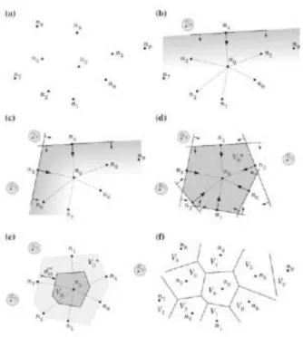
The outline respected by most meshless methods and the majority of other nodal dependent discretization numerical methods is as follows: first, it is necessary to study the problem geometry and establish the solid domain and the contour. Then, the essential and natural boundary conditions are identified, as it is possible to see in Figure 2.1a. Afterwards, as it is shown in Figure 2.1b and c, the problem domain and boundary is numerically discretized by a nodal set following a regular or irregular distribution.3
Figure 2.1 a.Problem domain with the essential and natural boundaries applied. b.Regular nodal discretization. c.Irregular nodal discretization3
7
Considering that it is not required, for meshless methods, any kind of previous information about the relation between the nodes towards the construction of the approximation (or interpolation) functions of the unknown variable field functions, the nodal distribution do not form a mesh. In fact, the only information necessary by truly meshless methods is the spatial location of each node discretized in the problem domain. The nodal discretization has a direct effect on the numerical analysis outcome and consequently, affects the method performance. An even nodal distribution as seen in Figure 2.1b leads, generally, to more accurate results and on the opposite, an uneven discretization of the nodes, Figure 2.1c, can often present lower accuracy. Despite this fact, locations with predictable stress concentrations, such as: domain discontinuities, crack tips, as seen in Figure 2.1 , among others, should present a higher nodal density when compared with locations in which smooth stress distributions are expected. In pursuance of solving both issues named before, it is possible to add extra nodes, only on the locations with predictable stress concentrations while maintaining a regular mesh on the rest of the problem domain, therefore, not increasing the computational cost significantly.3
Once it is obtained the problem domain discretization, it is now possible to get the nodal connectivity. While in FEM this is obtained using a predefined finite element mesh, in which it is known a priori which nodes belong to the same element and, consequently, interact directly between themselves. The boundary nodes interact with boundary nodes of nearby elements. On the other hand, in meshless methods, such connectivity is ensured by overlapping the influence-domains, when it comes to RPIM and influence-cells, when regarding NNRPIM.
Subsequently, it is created a background integration mesh, which can either be nodal dependent or independent, the later having a higher accuracy. The integration mesh can, at least, have the size of the problem domain, but in the cases in which it is larger, it cannot affect too much the final results. Afterwards, it is possible to obtain the field variables under study by using either approximation or interpolation shape functions, based on the combination of Radial Basis Functions (RBF) with polynomial basis functions.3
2.2 RPIM Formulation
2.2.1. Influence-domains and nodal connectivity
After the initial nodal discretization of the problem domain, it is necessary to impose the nodal connectivity between each and every node.
In order to find the nodal connectivity it is necessary to overlap the influence-domain of each node. The influence-domains are obtained through a process in which, firstly, it is settled an area (in case the problem is 2D) or a volume (in case the problem is 3D). Then, it is necessary to search for a specified number of nodes inside the previously established zone. As it is possible
8
to observe in Figure 2.2, there are influence-domains with different size and shape. Yet, the variation of this parameters along the problem domain affects the performance and the final solution of the meshless method. This said, it is important that all the influence-domains in the problem contain approximately the same number of nodes. Irregular domain boundaries or node clusters in the nodal distribution can lead to unbalanced influenced-domains. Regardless the used meshless technique, according to the literature, it is recommended using between n=[9,16] nodes for 2D problems and n=[27,70] nodes for 3D problems.7,11,15–17
Figure 2.2 Influence-domains with different sizes and shapes3
The number of nodes inside each influence-domain does not depend on the density of the nodal discretization and once selected, the value is valid for all domain discretization within the same analysis.
2.2.2. Numerical Integration
Based on the RPIM, a new meshless method has recently proven better results than other meshless RPIM approaches based on Gauss-Legendre integration schemes. Even though using a stabilized nodal integration, the extra time spent in this process does not pay the increased accuracy of the final solution.11,18 This said, in RPIM, the differential equations are integrated
using the Gauss-Legendre integration scheme. In order to ensure this, firstly, a background mesh is created. The connection of the nodes discretizing the problem domain gives origin to cells. These are the ones that will later compose the background mesh.
9
Figure 2.3 a.Fitted Gaussian background mesh. b.General Gaussian integration mesh.3
This mesh can either fit the solid-domain, as seen in Figure 2.3a, where no pos-treatment is needed, or, as it is possible to see in Figure 2.3b, be larger than the solid domain. In the latter case, the points outside the solid domain have to be removed.3
After all the solid domain is divided in a regular grid, each grid-cell is filled with integration points respecting the Gauss-Legendre quadrature rule. Taking as example Figure 2.4a, it is represented one grid-cell of the total background mesh. The initial quadrilateral is transformed in an isoparametric square, as seen in Figure 2.4b. Then, the Gauss-Legendre quadrature points are distributed inside the isoparametric square, and, in this case, it was used a 2x2 quadrature, Figure 2.4b.19,20
Figure 2.4 a.Initial grid-cell. b.Isoparametric square with integration points. c.Initial quadrature cell with integration points3
Later, with the intention to obtain the Cartesian coordinates of the quadrature points, isoparametric interpolation functions were used, and the results is the one presented in Figure 2.4c. The integration weight of the quadrature point is obtained multiplying the isoparametric weight of the quadrature point with the inverse of the Jacobian matrix determinant of the respective grid-cell.3 The following tables display the location and the weights of the
isoparametric integration points for quadrilateral and triangular element background meshes, respectively.
10
Table 2.1 Integration points coordinates and weights for quadrilateral ‘cells’.
Points ξ η Weight Representation
1 0 0 4 a − 1 √3 − 1 √3 1 b + 1 √3 − 1 √3 1 c − 1 √3 + 1 √3 1 d + 1 √3 + 1 √3 1 a −√3 5⁄ −√3 5⁄ 25 81 b 0 −√3 5⁄ 40 81 c +√3 5⁄ −√3 5⁄ 25 81 d −√3 5⁄ 0 40 81 e 0 0 64 81 f +√3 5⁄ 0 40 81 g −√3 5⁄ +√3 5⁄ 25 81 h 0 +√3 5⁄ 40 81 i +√3 5⁄ +√3 5⁄ 25 81
Table 2.2 Integration points coordinates and weights for triangular ‘cells’.
Points ξ η Weight Representation
a 13 13 12
a 16 16 16
OR
b 23 16 16
11 a 13 13 −27 96 b 15 15 2596 c 35 15 2596 d 15 35 2596
2.3 NNRPIM Formulation
2.3.1. Natural Neighbours
First introduced in 1980, as a way to obtain influence-cells, the concept of natural neighbours was created and is used by the NNRPIM, in order to determine the nodal connectivity. In opposition to the RPIM, which relies on the use of influence-domains.21 The
influence-cells are determined based on the geometric and spatial relations between the Voronoï cells, obtained from the Voronoï diagram of the nodal distribution. This concept was firstly introduced by Sibson for data fitting and field smoothing.12
Initially it is necessary to consider a nodal set, N, discretized in the space domain Ω ∈ ℝ2,
𝑁 = {𝑛1, 𝑛2, … , 𝑛𝑁}, and also 𝑋 = {𝑥1, 𝑥2, … , 𝑥𝑋}. The Voronoï diagram of N is the assembly of i
sub-regions Vi, closed and convex, in which, each sub-region is associated to the node ni in a
way that any point in the interior of Vi is closer to ni than any other node nj.3
𝑉𝑖= {𝑥𝐼 ∈ ℝ2: ‖𝑥𝐼− 𝑥𝑖‖ < ‖𝑥𝐼− 𝑥𝑗‖, ∀𝑖 ≠ 𝑗} (eq. 2.1)
being ‖. ‖ the distance between xI, an interest point and the nodes with coordinates defined
by xi e xj. Thus, the Voronoï diagram is defined by:
𝑉 = {𝑉1, 𝑉2, … , 𝑉𝑁} (eq. 2.2)
In Figure 2.5a, it is represented a nodal set in a two-dimensional space. Considering that the purpose is to determine the Voronoï cell V0 of the node n0, initially, it is necessary to choose
12
Figure 2.5 a.Initial nodal set. b.First trial plane. c.Second trial plane. d.Provisional Voronoï cell. e.Voronoï cell from node n0. f.Voronoï diagram.3
The nodes that are not included in the provisional selection are discarded. After this step, one of the nodes is selected as potential neighbour, for instance node n4, as seen in Figure
2.5b, it determined a vector u40.
𝑢40= (𝑥0−𝑥4)
‖𝑥0−𝑥4‖ (eq. 2.3)
In which 𝑢40= {𝑢40, 𝑣40, 𝑤40}. Afterwards a plane is defined. All the nodes that do not
respect the following condition are discarded:
𝑢40𝑥 + 𝑣40𝑦 + 𝑤40𝑧 ≥ (𝑢40𝑥4+ 𝑣40𝑦4+ 𝑤40𝑧4) (eq. 2.4)
This procedure is repeated for each and every node of the initial set of nodes, as it is possible to observe in Figure 2.5c. In Figure 2.5d, it is represented all of the 6 natural neighbours of node n0, and it is possible to see that nodes n7, n8 and n9 does not belong to the
referred cluster, because they do not respect the equation 2.4, mentioned before.3
Having already obtained the provisional Voronoï cell, it is now possible to obtain a definitive one, as shown in Figure 2.5e. The distance between node n0 and the boundary of the Voronoï
cell, V0 is half of node’s n0 and the neighbour node in question Euclidian norm. So, this distance
is given by the following equation:
𝑑0𝑖∗ = 𝑑0𝑖
2 = ‖𝑥0−𝑥𝑖‖
13
In order to obtain the remaining Voronoi cells, a similar procedure is applied, as seen in Figure 2.5f.3
2.3.2. Influence-Cells and Nodal Connectivity
As mentioned before in this work, in meshless methods, the nodal connectivity is obtained by overlapping the influence-domains of each interest point. In order to respond to difficulties that can affect the efficiency of the meshless methods when using blind influence-domains, the concept of influence-cells was created.22
Figure 2.6 a.First degree influence-cell. b.Second degree influence-cell.3
Regarding the level of nodal connectivity, influence-cells can be either “First degree influence-cells” or “Second degree influence-cells”, as seen in Figure 2.6a and 2.6b, respectively. According to the literature, “First degree influence-cells” are composed by only these natural neighbours and “Second degree influence-cells” contain, not only the first degree natural neighbour of a certain point of interest, but also, the natural neighbours of all the nodes belonging to the first degree of influence cells. Thus, the first degree influence-cell is naturally smaller than the second degree influence-cell. Therefore, as expected, the use of second degree influence-cells generally leads to better numerical results.
2.3.3. Numerical Integration
The Natural Neighbour Radial Point Interpolation Method (NNRPIM) uses a nodal based integration scheme proposed by Belinha and co-workers3 The most important advantage of this
scheme is that the background integration scheme is constructed using uniquely the nodal distribution spatial information. Since there is no information besides the spatial location of
14
the nodes discretizing the problem domain, is also necessary to: establish the nodal connectivity, determine the integration points and construct the shape functions. Hence, following the construction of the Voronoï diagram, it is possible to obtain a nodal dependent integration mesh based purely on the nodal distribution spatial information.
In order for this to be done, it is necessary to divide each of the Voronoï cells of the previously obtained Voronoï diagram and divide them into smaller sub-cells.
Figure 2.7 a.Voronoï cell and respective intersection points (PIi). b.Middle points (MIi) and the
respective generated quadrilaterals. c.Quadilateral3
In Figure 2.7a is possible to observe a constructed Voronoï cell, VI, of node nI, based on its
natural neighbours. Afterwards, the corners PIi of the polygonal shape defined by VI are
determined, Figure 2.7a. Then, the middle points, MIi, between nI and each neighbour node, ni
are obtained, Figure 2.7b. Hence, the Voronoï cells are divided in n quadrilateral sub-cells, SIi,
in which n is the number of natural neighbours of node nI, as seen in both Figure 2.7b and 2.7c.
If the N nodes discretizing the problem domain are irregularly scattered, the sub-cells that are originated are quadrilateral, on the other hand, if the field nodes N discretizing the problem domain are scattered in a regular nodal distribution, the Voronoï cells are divided in triangles, as sub-cells, instead of quadrilateral, as seen in Figure 2.8.
Figure 2.8 a.Voronoï cell and respective intersection points (PIi). b.Middle points (MIi) and the
respective generated quadrilaterals. c.Quadilateral3
The procedure to obtain sub-cells in case of a regular discretization of the problem domain is the same mentioned previously for the case of an irregular discretization of the problem domain. Due to the fact that it is always possible to divide a Voronoï cell, VI, in n sub-cells, SIi,
15
being n the total number of natural neighbours of ni, therefore, the area of the Voronoï cell,
VI, can be determined using the area of the n sub-cells SIi:
𝐴𝑉𝐼= ∑ 𝐴𝑆𝐼𝑖, ∀𝐴𝑆𝐼𝑖 ≥ 0
𝑛
𝑖=1 (eq. 2.6)
In which, 𝐴𝑉𝐼 is the area of the Voronoï cell VI and 𝐴𝑆𝐼𝑖 is the area of the sub-cell SIi.
In order to obtain the simplest integration scheme that can be established, using sub-cells with either triangular or quadrilateral shape, a single integration point is placed in the barycentre of the sub-cells. Consequently, spatial location of each integration point is determined on each sub-cell, Figure 2.9, being the weight of each integration point the area of the respective sub-cell.
The example pictured below only uses 1 integration point in each cell. However, it is possible to add more integration points.
Figure 2.9 Triangular and quadrilateral shapes and the respective integration points.3
Regarding this subject, initially, the sub-cell is divided again, although this time only as quadrilaterals, as seen in Figure 2.10, then, it is possible to apply the Gauss-Legendre quadrature to the obtained sub-quadrilaterals in order to obtain the integration points.19,20
Figure 2.10 Division in quadrilaterals of the sub-cells3
Afterwards, the process follows as it was described, in section 2.2.2, for the RPIM using quadrilateral integration. The resultant integration is as follows, in Figure 2.11.
16
Figure 2.11 Triangular and rectangular shape and respective integration points, xI, using the
Gauss-Legendre integration scheme.3
In Figure 2.11 are shown distinct integration schemes for the triangular and the quadrilateral sub-cells. Nevertheless, adding more integration points does not increase significantly the solution accuracy and, in addition, greatly increases the computational cost.3
Therefore, this work follows the suggestion from Belinha3 and only uses one integration point
per sub-cell. The domain integration mesh is obtained by repeating this process for the remaining Voronoï cells.
2.4 Shape Functions
Since the shape functions construction methodology should be able to use only the nodes discretizing the domain without the need of any pre-established mesh providing the nodal connectivity, its construction and development assume great importance in meshless methods.7
Both RPIM and NNRPIM use the same shape functions, based on a combination of radial basis functions with polynomial functions. The combination of these functions eliminates some issues such as the possible singularities created by methods that only use polynomial functions.11,18
One of the biggest advantages of both these method’s shape functions is that they possess the Kronecker delta property, meaning that they are interpolating shape functions.
First of all, it is necessary to consider an influence domain that has a set of arbitrarily distributed nodes 𝑃𝑖(𝑥𝑖) (𝑖 = 1,2, … , 𝑛), being n the number of nodes in the influence domain of
x and consider, also, a shape function (in this case, approximation function) u(x) in the referred
influence domain. Radial PIM constructs the approximation functions u(x) to pass through all these node points using radial basis function (RBF), Bi(x), and polynomial basis function,
Pj(x).11,18
Thus,
17
In equation 2.7, ai is the coefficient for Bi(x), and bj is the coefficient for Pj(x). Moreover,
n is the number of nodes in an domain of x, m is the polynomial term which is usually 𝑚 < 𝑛.
In equation 2.8 are defined the vectors
𝑎 = [𝑎1, 𝑎2, 𝑎3, … , 𝑎𝑛]𝑇, 𝑏 = [𝑏1, 𝑏2, 𝑏3, … , 𝑏𝑚]𝑇, 𝐵𝑇= [𝐵 1(𝑥), 𝐵2(𝑥), 𝐵3(𝑥), … , 𝐵𝑛(𝑥)], 𝑃𝑇 = [𝑃 1(𝑥), 𝑃2(𝑥), 𝑃3(𝑥), … , 𝑃𝑚(𝑥)], (eq. 2.8)
Above is defined the radial basis function, which is a function of distance r:
𝐵𝑖(𝑥) = 𝐵𝑖(𝑟𝑖)
𝑟𝑖= √[(𝑥 − 𝑥𝑖)2+ (𝑦 − 𝑦𝑖)2]
(eq. 2.9)
The monomial terms of the polynomial basis functions are as follows:
𝑃𝑇(𝑥) = [1, 𝑥, 𝑦, 𝑥2, 𝑥𝑦, 𝑦2, … ] (eq. 2.10)
The radial term transforms a multidimension into one-dimension, and the polynomial term improves the polynomial accuracy of the interpolation. According to Wang et al18 and his
research, addition of polynomial terms does not improve greatly the accuracy for non-polynomial functions, but it was revealed that there was no guarantee that the interpolating condition could be satisfied without the addition of polynomial terms.
Additionally, the coefficients should be constrained in order to assure the uniqueness of the interpolation. Constrains presented in equation 2.11 are usually imposed:
∑𝑛𝑖=1𝑃𝑗(𝑥𝑖, 𝑦𝑖)𝑎𝑖= 0, 𝑗 = 1,2, … , 𝑚 (eq. 2.11)
It can be expressed in matrix form, as follows:
[𝐵0 𝑃0 𝑃0𝑇 0 ] {𝑎𝑏} = {𝑢𝑒 0} 𝑜𝑟 𝐺 { 𝑎 𝑏} = { 𝑢𝑒 0} (eq. 2.12)
The distance is directionless, 𝐵𝑘(𝑥𝑖, 𝑦𝑖) = 𝐵𝑖(𝑥𝑘, 𝑦𝑘). If the inverse of the matrix G exists,
consequently, it is possible to obtain a unique solution:
{𝑎𝑏} = 𝐺−1{𝑢𝑒
18
As result, the interpolation is expressed as:
𝑢(𝑥) = [𝐵𝑇(𝑥)𝑃𝑇(𝑥)]𝐺−1{𝑢𝑒
0} = 𝜑(𝑥)𝑢
𝑒 (eq. 2.14)
Being 𝜑(𝑥) the shape function defined by:
𝜑(𝑥) = [𝛷1(𝑥), 𝛷2(𝑥), … , 𝛷𝑖(𝑥), … , 𝛷𝑛(𝑥)] (eq. 2.15)
Since shape functions from both RPIM and NNRPIM, as already said, respect the Kronecker delta property,
𝜑𝑖(𝑥𝑗) = {
1, 𝑖 = 𝑗, 𝑗 = 1,2, … , 𝑛
0, 𝑖 ≠ 𝑗, 𝑗 = 1,2, … , 𝑛 (eq. 2.16)
This means they pass through every single node within the domain (or influence-cell), in opposition to approximation shape functions which do not. When comparing approximation shape functions to interpolation shape function, the latter ones have reduced computational costs associated, due to using direct imposition methods, which allows to easily impose the essential and natural boundary conditions.11,18
Chapter 3
Solid Mechanics Fundamentals
Solids and structures subjected to loads or forces become stressed. The stresses lead to strains, which can be interpreted as deformations or relative displacements. Solid mechanics aim is to understand the relationship between stress and strain, as well as, the relationship between strain and displacements.3 Depending on the solid material stress-strain curve, solids
can show different behaviours.
In the present work, all solids were considered as being linear-elastic, it means that the relationship between stress and strain is assumed to be linear and after the removal of the applied load, the solid returns to its undeformed shape. Additionally, since this is a static study, only static loads were applied and considered, meaning that stresses, strains and displacements are not considered as a function of time.
Also, there are anisotropic and isotropic materials. The first ones are materials in which the properties varies with the directions. On this type of materials the deformation caused by a load applied in a certain direction is different from the deformation caused by the same load applied in a different direction. Isotropic materials are a special case of anisotropic materials, since only two independent material properties need to be known, the Young modulus (E) and the Poisson ratio (ν). In this work, only isotropic material were used.3
3.1 Stress Components
Due to the application of external loads, internal forces are produced. As represented in equation 3.1, these internal forces are defined by the variation of force per unit of area and are entitled stress.
𝑇 = lim
∆𝐴→0 ∆𝐹
20
On a certain point, the stress a body is under is given by the following stress tensor:
𝜏 = [
𝜎𝑥𝑥 𝜏𝑥𝑦 𝜏𝑥𝑧
𝜏𝑦𝑥 𝜎𝑦𝑦 𝜏𝑦𝑧
𝜏𝑧𝑥 𝜏𝑧𝑦 𝜎𝑧𝑧
] (eq. 3.2)
This tensor can also be written as a vector:
𝜎 = {𝜎𝑥𝑥𝜎𝑦𝑦𝜎𝑧𝑧𝜏𝑥𝑦𝜏𝑦𝑧𝜏𝑧𝑥}T (eq. 3.3)
Stress can be divided into two categories, normal stress, which is perpendicular to the plane in question, denotes by the letter σ and shear stress, which is tangential to the plane in which it acts, denoted by the letter τ.23
3.2 Equilibrium equations
Although stresses vary according to the volume of the body, these cannot vary randomly between two given points. An infinitesimal element is characterized by three dimensional equilibrium equation, which are:
𝜕𝜎𝑥𝑥 𝜕𝑥 + 𝜕𝜏𝑦𝑥 𝜕𝑦 + 𝜕𝜏𝑧𝑥 𝜕𝑧 + 𝐹𝑥 = 0 𝜕𝜏𝑥𝑦 𝜕𝑥 + 𝜕𝜎𝑦𝑦 𝜕𝑦 + 𝜕𝜏𝑧𝑦 𝜕𝑧 + 𝐹𝑦= 0 𝜕𝜏𝑥𝑧 𝜕𝑥 + 𝜕𝜏𝑦𝑧 𝜕𝑦 + 𝜕𝜎𝑧𝑧 𝜕𝑧 + 𝐹𝑧= 0 (eq. 3.4)
And must be verified for every point throughout the volume of the body.23
3.3 Components of strain
Due to the fact that no material is perfectly rigid, when subject to external loads, a body will become deformed. Regarding the deformable body presented in Figure 3.1, prior to applying any external loads, point Q was in a certain space location, but as soon as external loads are applied, this leads to a change on the location giving origin to any point location, q.
21
Figure 3.1 Linear deformation of a virtual body3
The equation that defines the displacement field, for any given point of the solid is:
𝑢(𝑢, 𝑣, 𝑤) = {
𝑢(𝑥, 𝑦, 𝑧) 𝑣(𝑥, 𝑦, 𝑧) 𝑤(𝑥, 𝑦, 𝑧)
} (eq. 3.5)
Strain and displacements are related according to the following equations,
𝜀𝑥𝑥 𝜕𝑢 𝜕𝑥 𝜀𝑦𝑦 𝜕𝑣 𝜕𝑦 𝜀𝑧𝑧 𝜕𝑤 𝜕𝑧 𝑌𝑥𝑦= 𝜕𝑣 𝜕𝑥+ 𝜕𝑢 𝜕𝑦 𝑌𝑦𝑧= 𝜕𝑤 𝜕𝑦+ 𝜕𝑣 𝜕𝑧 𝑌𝑧𝑥= 𝜕𝑢 𝜕𝑧+ 𝜕𝑤 𝑑𝑥 (eq. 3.6)
Similarly to what happens in stress, there is also two types of strain. The normal strain, which can be represented by the letter ε, and represents the relative change of length of a certain line segment. On the other hand, the shear strain is represented by the letter γ and refers to the change in angle of two previously perpendicular line segments.23
The strain tensor comes:
𝜀 = [
𝜀𝑥𝑥 𝛾𝑥𝑦 𝛾𝑥𝑧
𝛾𝑦𝑥 𝛾𝑦𝑦 𝛾𝑦𝑧
𝛾𝑧𝑥 𝛾𝑧𝑦 𝜀𝑧𝑧
] (eq.3.7)
The equations presented in 3.6 can be represented in matrix form as the product of the partial differential equation operator matrix L and the displacement field u.
𝜀 = 𝑳𝒖 (eq.3.8)
22 𝑳 = [ 𝜕 𝜕𝑥 0 0 𝜕 𝜕𝑦 0 𝜕 𝜕𝑧 0 𝜕 𝜕𝑦 0 𝜕 𝜕𝑥 𝜕 𝜕𝑧 0 0 0 𝜕 𝜕𝑧 0 𝜕 𝜕𝑦 𝜕 𝜕𝑥] 𝑻 ……. (eq. 3.9)
3.4 Constitutive equations
Due to all solids considered in this work were isotropic, besides the fact that not only is the material completely defined by just its Elastic Modulus and Poisson’s ratio, but also, by the components of stress and strain relation, which is given by the generalized Hooke’s Law.23
𝝈 = 𝒄 𝜺 (eq. 3.10)
In which, c is the constitutive matrix of the material, defined by:
𝒄 = 𝐸 (1+𝜈)(1−2𝜈) [ 1 − 𝜈 𝜈 𝜈 0 0 0 𝜈 1 − 𝜈 𝜈 0 0 0 𝜈 𝜈 1 − 𝜈 0 0 0 0 0 0 (1 − 2𝜈) 0 0 0 0 0 0 (1 − 2𝜈) 0 0 0 0 0 0 (1 − 2𝜈)] (eq. 3.11)
This constitutive matrix can also be obtained by inverting the compliance elasticity matrix, 𝑐 = 𝑠−1. In equations 3.12 and 3.13 are defined the plane stress and plane strain, respectively,
for the general anisotropic material case, the compliance elasticity matrix s.
𝑠𝑝𝑙𝑎𝑛𝑒 𝑠𝑡𝑟𝑒𝑠𝑠= [ 1 𝐸11 − 𝜈21 𝐸22 0 −𝜈12 𝐸11 1 𝐸22 0 0 0 1 𝐺12] (eq. 3.12) 𝑠𝑝𝑙𝑎𝑛𝑒 𝑠𝑡𝑟𝑎𝑖𝑛= [ 1−𝜈31𝜈13 𝐸11 − 𝜈12+𝜈31𝜈23 𝐸22 0 −𝜈12+𝜈32𝜈13 𝐸11 1−𝜈32𝜈23 𝐸22 0 0 0 1 𝐺12] (eq. 3.13)
being Eij the elastic modulus, νij the material Poisson coefficient and Gij the distortion
modulus in material direction i and j. It is possible to align the constitutive matrix c with a new material referential Ox’y’ defined by 𝑖′= {𝑖
𝑥′, 𝑖𝑦′} and 𝑗′= {−𝑖𝑦′, 𝑖𝑥′}, which are versors of the new
material referential. Hence,
23
where the transformation matrix T is defined by,
𝑇 = [
𝑐𝑜𝑠2 𝛼 𝑠𝑖𝑛2 𝛼 − sin 2𝛼
𝑠𝑖𝑛2 𝛼 𝑐𝑜𝑠2 𝛼 sin 2𝛼
sin 𝛼 ∙ cos 𝛼 − sin 𝛼 ∙ cos 𝛼 𝑐𝑜𝑠2𝛼 − 𝑠𝑖𝑛2𝛼
] (eq. 3.15)
the angle 𝛼 is the angle between the original material axis Ox and the new material axis 𝑂𝑥′: 𝛼 = cos−1(𝑖 ∙ 𝑖′).
3.5 Strong form and weak form formulation
The partial differential system equations are strong forms of the governing system of equations for solids. The strong form, in contrast to a weak form, requires strong continuity on the dependent field variables. Whatsoever functions that define these field variables have to be differentiable up to the order of the partial differential equations that exist in the strong form of the system. On the other hand, the weak form requires a weaker consistency on the adopted approximation (or interpolation) functions.
By reason of the weaker requirements on the field variables, and the integral operation, a formulation based on a weak form, usually produces a set of discretized system equations that give much more accurate results, especially for problems of complex geometry. These are the reasons why so many prefer the weak form to obtain the approximated solution. However, accuracy is dependent on the density of the mesh discretizing the problem domain.3,24
3.5.1. Galerkin weak form
The Galerkin weak form is a variational principle based on the energy principle. Between all possible displacement configurations satisfying the compatibility conditions, the essential boundary conditions and the initial and final time conditions, the real solution correspondent configuration in the one that minimizes the Lagrangian functional L,
𝐿 = 𝑇 − 𝑈 + 𝑊𝑓 (eq. 3.16)
Where T is the kinetic energy, U is the strain energy and Wf is the work produced by the
external forces.
The variables above can be replaced by the equations that defines them, which can be written as, 𝐿 =1 2∫ 𝜌
ů
𝑇 𝛺 ů 𝑑𝛺 − 1 2∫ 𝜀 𝑇𝜎 𝑑𝛺 + ∫ 𝑢𝑇𝑏 𝑑𝛺 + ∫ 𝑢𝑇𝑓 𝑑Г Г𝑡 𝛺 𝛺 (eq. 3.17)24
Where the solid volume is defined by Ω, ů is the displacement first derivative with respect to time and ρ is the solid mass density. ε is the strain vector and σ is the stress vector. Lastly,
u represents the displacement, b the body forces and Гt the traction boundary where the
external forces f are applied.
Minimizing equation 3.17, the following is obtained:
𝛿 ∫ [1 2∫ 𝜌
ů
𝑇 𝛺 ů 𝑑𝛺 − 1 2∫ 𝜀 𝑇𝜎 𝑑𝛺 + ∫ 𝑢𝑇𝑏 𝑑𝛺 + ∫ 𝑢𝑇𝑓 𝑑Г Г𝑡 𝛺 𝛺 ] 𝑑𝑡 = 0 𝑡2 𝑡1 (eq. 3.18)Moving the variation operator 𝛿 inside the integrals,
∫ [1 2∫ 𝛿(𝜌
ů
𝑇 𝛺 ů)𝑑𝛺 − 1 2∫ 𝛿(𝜀 𝑇𝜎)𝑑𝛺 + ∫ 𝛿𝑢𝑇𝑏 𝑑𝛺 + ∫ 𝛿𝑢𝑇𝑓 𝑑Г Г𝑡 𝛺 𝛺 ] 𝑑𝑡 = 0 𝑡2 𝑡1 (eq. 3.19)Due to the fact that in this work only static problems were considered, the first term of the equation 3.19 can be discard, which leads to:
∫ [−12∫ 𝛿(𝜀𝑇𝜎)𝑑𝛺 + ∫ 𝛿𝑢𝑇𝑏 𝑑𝛺 + ∫ 𝛿𝑢𝑇𝑓 𝑑Г Г𝑡 𝛺 𝛺 ] 𝑑𝑡 = 0 𝑡2 𝑡1 (eq. 3.20)
Considering the equation 3.20, there are some simplifications that can be made to the first term of the integral. The integrand function can be written as:
𝛿(𝜀𝑇𝜎) = 𝛿𝜀𝑇𝜎 + 𝜀𝑇𝛿𝜎 (eq. 3.21)
Since both terms are scalars, in equation 3.21,
𝜀𝑇𝛿𝜎 = (𝜀𝑇𝛿𝜎)𝑇 = 𝛿𝜎𝑇𝜀 (eq. 3.22)
According to the generalized Hooke’s law shown in 3.10, and the symmetric property of material shown in 3.11, 𝑐𝑇 = 𝑐, it is possible to write:
𝛿𝜎𝑇𝜀 = 𝛿𝜀𝑇𝜎 (eq. 3.23)
Hence, by replacing equation 3.23 in equation 3.21,
𝛿(𝜀𝑇𝜎) = 2(𝛿𝜀𝑇𝜎) ...(eq. 3.24)
Substituting equation 3.24 in equation 3.20
∫ [− ∫ 𝛿(𝜀𝑇𝜎)𝑑𝛺 + ∫ 𝛿𝑢𝑇𝑏 𝑑𝛺 + ∫ 𝛿𝑢𝑇𝑓 𝑑Г Г𝑡 𝛺 𝛺 ] 𝑑𝑡 = 0 𝑡2 𝑡1 …….(eq. 3.25)
25
If it is pretended for the time integration to be valid for any pair of initial and final time,
t1 and t2, respectively, the integrand from equation 3.25 must be null. This leads to the
“Galerkin weak form” equation,
− ∫ 𝛿𝜀𝑇𝜎𝑑𝛺 + ∫ 𝛿𝑢𝑇𝑏 𝑑𝛺 + ∫ 𝛿𝑢𝑇𝑓 𝑑Г Г𝑡
𝛺
𝛺 = 0 (eq. 3.26)
Replacing equations 3.8 and 3.10 In equation 3.26, the generic Galerkin weak form written in terms of displacement is obtained,
∫ 𝛿(𝑳 𝒖)𝑇𝒄 (𝑳 𝒖)𝑑𝛺 − ∫ 𝛿𝑢𝑇𝑏 𝑑𝛺 − ∫ 𝛿𝑢𝑇𝑓 𝑑Г Г𝑡
𝛺
𝛺 = 0 (eq. 3.27)
3.6 Discrete System Equations
Having as base the principle of virtual work, the discrete equations for meshless methods are obtained by using the meshless shape functions as trial and test functions. The meshless trial function u(xI) Is given by,
𝑢(𝑥𝑖) = ∑𝑛𝑖=1𝜑𝑖(𝑥𝐼)𝑢𝑖 (eq. 3.28)
in which 𝜑𝑖(𝑥𝐼) is the meshless approximation or interpolation function and 𝑢𝑖 are the nodal
displacements of the n nodes belonging to the influence-domain of interest node 𝑥𝑖.
It is known that the NNRPIM interpolation function satisfies the condition,
𝜑𝑖(𝑥𝑗) = 𝛿𝑖𝑗 (eq. 3.29)
Where 𝛿𝑖𝑗 is the Kronecker delta, being 𝛿𝑖𝑗= 1 𝑖𝑓 𝑖 = 𝑗 and 𝛿𝑖𝑗= 0 𝑖𝑓 𝑖 ≠ 𝑗.
Following equation 3.24, the test function (or virtual displacements) are defined as,
𝑑𝑢(𝑥𝑖) = ∑𝑛𝑖=1𝜑𝑖(𝑥𝐼)𝑑𝑢𝑖 (eq. 3.30)
Where 𝑑𝑢𝑖 are the nodal values for the test function.
Since that in the presented work it was studied only two-dimensional problems considering the plane strain or the plane stress assumptions, each node xi discretizing the problem domain
has two degrees of freedom: 𝑢𝑖= {𝑢𝑖, 𝑣𝑖}. Thus, in order to interpolate the virtual displacement