Human Activity Recognition for an Intelligent Knee Orthosis

(1)

Diliana Maria Barradas Rebelo dos Santos

Master’s in Biomedical Engineering

Human Activity Recognition for an Intelligent

Knee Orthosis

Dissertação para obtenção do Grau de Mestre em Engenharia Biomédica

Orientador :

Hugo Filipe Silveira Gamboa, Prof. Auxiliar,

Faculdade de Ciências e Tecnologias da

Uni-versidade Nova de Lisboa

Co-orientadores :

Christoph Amma, phD Student,

Cognitive Systems Lab, Karlsruhe Institute of

Technology, Germany

Tanja Schultz, Profª. Catedrático,

Cognitive Systems Lab, Karlsruhe Institute of

Technology, Germany and Carnegie Mellon

University, Pittsburg, USA

Júri:

Presidente: Doutor Pedro Manuel Cardoso Vieira

Arguente: Doutora Ana Luísa Nobre Fred

(2)

(3)

iii

Human Activity Recognition for an Intelligent Knee Orthosis

(4)

(5)

(6)

(7)

Acknowledgements

First and foremost, I offer my sincerest gratitude to my supervisor, Professor Hugo Gam-boa, who has supported me throughout my thesis with his patience and knowledge whilst allowing me the room to work in my own way. I attribute the level of my Masters degree to his encouragement and effort and without him this thesis, too, would not have been completed.

This project would not have been possible either without my stay in Karlsruhe, in

CSL-Cognitive Systems Labof theKIT-Karlsruhe Institute of Technologyunder Dr.Tanja Scultz’s

guidance. To you, Dr.Tanja Scultz, I thank you for the wonderful reception, environment and knowledge your laboratory offered me. To my co-supervisor, PhD student Christoph Amma, my biggest acknowledgement for the extreme patience to fulfil all of my ques-tions and needs, to polish my failures and to be available 24/7.

In my daily work I have been blessed with a friendly and cheerful group of fellow stu-dents. I would like to thank all of myCSL-friends, Mark, Thang, Dominic T., George, Tim,

Dario, Dirk, Dominic H., Christian, Matthias, Michael, Daniel L., Daniel, Lena, Zlatka, and every others and to my friend from India, Melvin, for making my time in Germany one of the best in my life. Back in Portugal, the daily presence of my dearest friends Rodolfo, Ângela, Ricardo and Nuno was crucial whether for the funny moments and ad-ventures or for the constant available support.

I shall thank you with all of my heart.

I also want to underline the primordial role of all of the excellency professionals from

PLUX-Wireless Biosignals, S.A., who welcomed me and supported me along my thesis.

(8)

(9)

Abstract

Activity recognition with body-worn sensors is a large and growing field of research. In this thesis we evaluate the possibility to recognize human activities based on data from biosignal sensors solely placed on or under an existing passive knee orthosis, which will produce the needed information to integrate sensors into the orthosis in the future.

The development of active orthotic knee devices will allow population to ambulate in a more natural, efficient and less painful manner than they might with a traditional orthosis. Thus, the term’active orthosis’refers to a device intended to increase the

ambu-latory ability of a person suffering from a knee pathology by applying forces to correct the position only when necessary and thereby make usable over longer periods of time.

The contribution of this work is the evaluation of the ability to recognize activities with these restrictions on sensor placement as well as providing a proof-of-concept for the development of an activity recognition system for an intelligent orthosis.

We use accelerometers and a goniometer placed on the orthosis and Electromyography (EMG) sensors placed on the skin under the orthosis to measure motion and muscle activ-ity respectively. We segment signals in motion primitives semi-automatically and apply Hidden-Markov-Models (HMM) to classify the isolated motion primitives. We discrim-inate between seven activities like for example walking stairs up and ascend a hill. In a user study with six participants, we evaluate the systems performance for each of the different biosignal modalities alone as well as the combinations of them. For the best performing combination, we reach an average person-dependent accuracy of 98% and a person-independent accuracy of 79%.

(10)

(11)

Resumo

O reconhecimento de actividade humana com sensores corporais é um vasto e pro-missor campo de investigação. Ao longo deste projecto de mestrado, avaliamos a possi-bilidade de reconhecimento de movimento humano através do estudo de biosinais cap-tados por sensores localizados directamente numa ortótese do joelho ou na pele, o que permitirá obter a informação necessária para se proceder à integração futura destes sen-sores no próprio dispositivo.

O desenvolvimento de dispositivos ortóticos activos do joelho proporcionará à po-pulação doente um meio de locomoção mais natural, eficiente e menos dolorosa quando comparado com os tradicionais. O termo’ortótese activa’refere-se ao dispositivo cuja

fun-ção é melhorar a capacidade de movimento de uma pessoa que sofre de uma patologia do joelho recorrendo à aplicação de uma força somente quando necessária o que leva ao seu uso por um maior período de tempo.

Este trabalho contribuirá para o desenvolvimento da área de reconhecimento de acti-vidade humana na vertente de possibilidade de criação de equipamentos médicos inteli-gentes com sensores incorporados.

Sob a ortótese, dispomos os acelerómetros e o goniómetro e, sob a pele, são colocados os eléctrodos de electromiografia de superfície de modo a captar movimento e activi-dade muscular, respectivamente. Quanto à metodologia, os sinais são repartidos semi-automáticamente em ciclos que, após a extracção de características, constituem a entrada para o classificador supervisionado escolhido,HMM. Num estudo desempenhado por seis participantes, investigámos qual o grau de identificação dos movimentos bem como qual ou quais as combinações de sinais com maior precisão. Para a melhor combina-ção, obtivémos um rigor de 98% num contexto sujeito-dependente e 79% para o caso de sujeito-independente.

(12)

(13)

List of Figures

1.1 Thesis’ overview diagram . . . 2

2.1 Knee anterior (A) and posterior (B) view [1] . . . 6

2.2 Superior end of the right tibia [1] . . . 6

2.3 Knee supporting structures diagram [1] . . . 7

2.4 Knee extensors and flexors muscles [2, 3]. . . 8

2.5 X-ray of a normal knee with space between the bone of the upper and lower leg (A). (B) shows bone spurs and a narrowed joint space caused by osteoarthritis [4] . . . 9

2.6 Signal classification . . . 10

2.7 EMG acquisition, with an electrode placed on the skin, and example of a raw signal [5] . . . 11

2.8 The figure represents two goniometers from Biometrics Ldt. . . 12

2.9 Accelerometer axis representation and acquired signals [6]. This pictures also shows the sensors’ length (L), width (W) and height (H).. . . 12

2.10 Classification theory scheme . . . 13

2.11 HMM model with left-to-right topology with three emissors states [7]. . . 15

3.1 Standard right knee Ortema ipomax passive orthosis . . . 18

3.2 Complete experimental setup: two Bioplux research devices, two ACC (red circles), six EMG and one GON sensors (green arrow) placed on a regular Ortema right knee orthosis . . . 19

3.3 Placement of EMG surface electrodes. . . 19

3.4 Goniometer and the device attached to the orthosis . . . 20

3.5 Principal bones of the knee joint [8] . . . 21

3.6 Placement of the ACC sensors . . . 21

(16)

xvi LIST OF FIGURES

4.1 EMG raw signals for the sequence walk and walk stairs up. Plot shows quadriceps’, hamstrings’ and gastrocnemius’ activity, from top to bottom. 26 4.2 GON raw signal for the sequence walk and walk stairs up. Plot shows how

the range of motion evolutes over time for theyaxis . . . 26

4.3 ACC raw signals for the sequence walk and walk stairs up. Plot shows femur’s(x, y, x) and tibia’s(x, y, z)acceleration, respectively, from top to

bottom . . . 26 4.4 Representative scheme for the automatic segmentation algorithm. The

sig-nals refer to the movementwalk . . . 27

4.5 One cycle for walking based on the analysis of the goniometer output. . . 28 4.6 One cycle for walking stairs up based on the analysis of the goniometer

output . . . 28

6.1 Classification accuracy per combination of signals in a subject’s dependent case . . . 36 6.2 Classification accuracy per subjects for Goniometry and Accelerometry

(GON&ACC) set in a subject’s dependent case . . . 38 6.3 Classification accuracy per combination of signals in a subject’s

indepen-dent case . . . 39 6.4 Classification accuracy per subjects for GON&ACC in a subject’s

indepen-dent case . . . 42

(17)

List of Tables

3.1 Means and standard deviations of the anthropometric characteristics of all subjects . . . 17

4.1 Number of isolated cycles from all subjects for each movement from all original acquired data . . . 29 4.2 Number of isolated cycles from all subjects for each movement randomly

selected for a balanced database. . . 29

6.1 Classification accuracy (mean and standard deviation) per combination of signals in a subject’s dependent case . . . 36 6.2 Confusion matrix for EMG set in a subject-dependent context (in percentage) 36 6.3 Confusion matrix for GON set in a subject-dependent context (in percentage) 37 6.4 Confusion matrix for ACC set in a subject-dependent context (in percentage) 37 6.5 Confusion matrix for Electromyography and Goniometry (EMG&GON)

set in a subject-dependent context (in percentage) . . . 37 6.6 Confusion matrix for GON&ACC set in a subject-dependent context (in

percentage). . . 37 6.7 Confusion matrix for Electromyography and Accelerometry (EMG&ACC)

set in a subject-dependent context (in percentage) . . . 38 6.8 Confusion matrix for Electromyography, Goniometry and Accelerometry

(EMG&GON&ACC) set in a subject-dependent context (in percentage) . . 38 6.9 Classification accuracy (mean and standard deviation) per subject for GON&ACC

set in a subject’s dependent case . . . 39 6.10 Classification accuracy (mean and standard deviation) per combination of

signals in a subject’s independent case . . . 39 6.11 Confusion matrix for EMG set in a subject-independent context (in

per-centage). . . 40 6.12 Confusion matrix for GON set in a subject-independent context (in

(18)

xviii LIST OF TABLES

6.13 Confusion matrix for ACC set in a subject-independent context (in per-centage). . . 40 6.14 Confusion matrix for EMG&GON set in a subject-independent context (in

percentage) . . . 41 6.15 Confusion matrix for GON&ACC set in a subject-independent context (in

percentage) . . . 41 6.16 Confusion matrix for EMG&ACC set in a subject-independent context (in

percentage) . . . 41 6.17 Confusion matrix for EMG&GON&ACC set in a subject-independent

con-text (in percentage) . . . 41 6.18 Classification accuracy (mean and standard deviation) per subject for GON&ACC

(19)

Listings

ACC Accelerometry

EMG Electromyography

GON Goniometry

HMM Hidden-Markov-Models

GMM Gaussian Mixture Model

MCL Medial Collateral Ligament

LCL Lateral Collateral Ligament

ACL Anterior Collateral Ligament

PCL Posterior Collateral Ligament

ROM Range of Motion

EM Expectation Maximization

MCFS Multi Channel Feature Sequence

FS Feature Sequence

EMG&GON Electromyography and Goniometry

GON&ACC Goniometry and Accelerometry

EMG&ACC Electromyography and Accelerometry

EMG&GON&ACC Electromyography, Goniometry and Accelerometry

ECG Electrocardiography

(20)

(21)

1

Introduction

1.1 Motivation

Passive orthoses are widely used for conservative therapy of diseases like Gonarthrosis, which is Osteoarthritis in the knee joint. Depending on the type of arthrosis, these or-thoses apply a constant force on the knee joint to correct a defective position. This is usually painful or at least unpleasant for the wearer after a certain amount of time. Fu-ture active orthoses could be able to vary this force depending on the current wearers activity and therefore only apply force if the knee joint is stressed, e.g. while walking stairs but not while the wearer is sitting. This will impose less strain on the wearer. In order to develop such an active orthosis it is necessary to robustly recognize the users activity, which is the topic of this thesis.

Briefly, we can summarize the motivation of this work in two questions:

• How can we improve the patient’s daily life quality?

• How can we rely on biomechanical signals for human activity recognition?

1.2 Objectives

(22)

1. INTRODUCTION 1.3. Thesis Overview

objective of this thesis is to state which signal (or combination of signals) provide higher classification accuracy.

In order to fulfill these goals, we used a methodology based on pattern recognition andHMMas classifier. The procedure is explained on chapters5and6.

The contribution of this work is the evaluation of the ability to recognize activities with these restrictions on sensor placement as well as providing a proof-of-concept for the development of an activity recognition system for an intelligent orthosis.

1.3 Thesis Overview

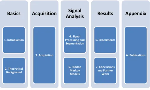
This thesis is organized in seven chapters and one appendix, as represented in figure1.1.

Basics

1. Introduction 2. Theoretical Background

Acquisition

3. Acquisition

Signal

Analysis

4. Signal Processing and Segmentation 5. Hidden Markov Models

Results

6. Experiments 7. Conclusions and Further Work

Appendix

A. Publications

Figure 1.1: Thesis’ overview diagram

This first chapter introduces the theme and motivation to the reader, explaining the objectives and importance of the developed work. It has the goal to contextualize the reader giving a thesis overview. Next, in Chapter2, the theoretical concepts are presented as well as the state of the art. These two chapters form the basic structure for the overall work.

The second block consists in just one chapter, Acquisition, where the procedure for

signal recording is detailed. Each one of the six subjects hadEMGsensors placed on the skin and wore a passive orthosis withGONandACCsensors placed on it and performed the activities’ acquisition protocol. This chapter concerns the collection of data.

Chapter 4 discusses the acquired raw signals and clarify the algorithm for semi-automatic segmentation. Plus, the total structure of our final database is presented. In Chapter5theHMMdecoding used in this project is introduced as well as the main dif-ferences compared to a standardHMM. These two chapters fix up the third block named

(23)

1. INTRODUCTION 1.3. Thesis Overview

The Results set consists of chapter 6 and chapter 7. Chapter 6 presents a detailed

description of the performed experiments together with a discussion of the results. As a continuation, chapter7resumes our work by presenting the main conclusions and further work.

The thesis has one additional appendix which contains the papers published during this project:Clustering Algorithm for Human Behaviour Recognition based on Biosignals Anal-ysis, accepted as a book chapter in Human Behaviour Recognition Technologies: Intelligent Applications for Monitoring and Security andHuman Activity Recognition for an Intelligent Knee Orthosissubmitted to the2013 Biosignals Conference.

The implemented algorithms were develop usingPython,Eclipseand theBioKit

(24)

(25)

2

Theoretical Background

The purpose of this chapter is to contextualize the reader about the main subject of this work. Through the subchapters, we will introduce the knee anatomy, biomechanical signals acquisition and processing, classification algorithms and literature review.

2.1 Knee Anatomy

2.1.1 Essential Concepts

The knee joint combines several bones, muscles and ligaments. As a short approach, it integrates three bones: femur, which is the thigh large bone attached by ligaments to the

tibiaand thepatella(or kneecap), that slides on the knee as it bends (see figures2.1,2.2and

2.3). There are also a number of ligaments, cartilages and muscles which strengthen and support the knee [1]. Basically, the knee can be thought of having four ligaments which stabilize it [1]:

1. Medial Collateral Ligament (MCL): Runs along the inner part of the knee and pre-vents bending inwards;

2. Lateral Collateral Ligament (LCL): Runs along the outer part of the knee and pre-vents bending outwards;

3. Anterior Collateral Ligament (ACL): Lies in the middle of the knee and prevents the tibia sliding forwards in front of the femur. It also provides rotational stability;

(26)

2. THEORETICALBACKGROUND 2.1. Knee Anatomy

Meniscus

The meniscus is a wedge-like cushion which connects the bones of the knee together. The cartilages are shaped in a form that provides a strong stabilization. It helps the weight support and it also interferes in sliding and turning in many direction. It also acts as a shock absorber and keeps the thigh bone and shin bones from grinding against

each other.Changed with the DEMO VERSION of CAD-KAS PDF-Editor (http://www.cadkas.com).Changed with the DEMO VERSION of CAD-KAS PDF-Editor (http://www.cadkas.com).Changed with the DEMO VERSION of CAD-KAS PDF-Editor (http://www.cadkas.com).

Figure 2.1: Knee anterior (A) and posterior (B) view [1]

(27)

Capsular arm

Tibial arm

Tibial collateral ligament

Direct insertion semimenbranosus

Superficial arm posterior oblique ligament

Semimembranosus

Capsular arm semimembranosus

Pars reflexa

Medial head of gastrocnemius

Changed with the DEMO VERSION of CAD-KAS PDF-Editor (http://www.cadkas.com).Changed with the DEMO VERSION of CAD-KAS PDF-Editor (http://www.cadkas.com).Changed with the DEMO VERSION of CAD-KAS PDF-Editor (http://www.cadkas.com).

Figure 2.3: Knee supporting structures diagram [1]

2.1.2 Muscles

2.1.2.1 Quadriceps: Extensor muscles

The extensor knee muscle group is the quadriceps. As the name suggests, it has four

"components":anterior rectum,vastus lateralis,vastus medialisandvastus intermedius, which

converge to a distal insertion at the patella and tibia’s anterior tuberosity. Quadriceps are responsible for knee extension.Thevastus medialisis responsible for medial rotation and, vastus lateralisfor lateral rotation [9].

2.1.2.2 Hamstring: Flexor muscles

Hamstringis the muscle complex responsible for flexion. It consists of a combination of

three small but long muscles:femoral biceps,semitendinosusandsemimembranosusmuscles

[9].

Femoral biceps It begins at the ischial tuberosity and at the lateral lip of the linea aspera of the femur converging to the fibular head. This muscle performs extension by adduction and external rotation and, flexion by external rotation of the knee. It also provides pelvic retroversion.

Semitendinosus muscleSemitendinosus muscle also begins at the ischial tuberosity next to the femoral biceps and converges to the tibial tuberosity. It is responsible for hip extension, helps in internal rotation and adduction as well as performing flexion and medial rotation of the knee. If the lower limbs are fixed, semitendinosus muscle provides pelvis retroversion.

Semimembranosus muscleAnalogously to femoral biceps and semitendinosus

(28)

insertion is in the proximal tibia by fascia of the popliteal muscle. It performs extension, adduction and hip internal rotation as well as flexion and internal rotation of the knee.

2.1.2.3 Gastrocnemius: Flexor muscle

The gastrocnemius is a large muscle located in the lower leg forming part of the calf and participates directly on the flexion of the knee. Its purpose is to push the leg down when required during activities such as walking, jogging or even just standing. It also allows plantar flexion of the foot, which is important in a number of different activities.

The gastrocnemius originates toward the bottom of the femur and inserts at the Achilles tendon.

The figure2.4illustrates all of the three muscle complexes aforementioned.

Gastrocnemius

Biceps Femoris

Semi-membranosus

Semi-tendinosus Vastus Intermedius and Rectus Femoris

Vastus Lateralis

Vastus Medialis

Figure 2.4: Knee extensors and flexors muscles [2,3]

2.1.3 Pathology: Gonarthrosis

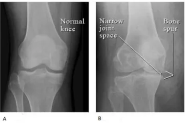
Osteoarthritis is a joint inflammation that results from cartilage degeneration and it can be caused by aging, heredity and injury from trauma or disease. This pathology is de-generative and it can be characterized by the progressive destruction of joint cartilage, bone sclerosis and osteochondral proliferation, which results in a painful movement or progressive functional movement impotence.

Gonarthrosis is osteoarthritis in the knee.

(29)

2. THEORETICALBACKGROUND 2.2. Introduction to biosignals

Figure 2.5: X-ray of a normal knee with space between the bone of the upper and lower leg (A). (B) shows bone spurs and a narrowed joint space caused by osteoarthritis [4]

2.2 Introduction to biosignals

Biosignal monitoring and recording is the extension of medical investigations taking into consideration the development over time. A biosignal is a term applied to all signals continuously captured from biological sources. Each kind may be related to a specific event so they are usually categorized as [10–12]:

• Bioelectrical signals: Bioelectric signals are formed in cells and organs by nerve cells, mainly in the heart and the brain. Its source is the cell membrane and it propagates as an action potential. They are very low amplitude and low frequency;

• Biomechanical signals:This type represents all signals from some biological move-ment source such as motion, force, pressure or flow;

• Biomagnetic signals: The concept of biomagnetic signals is inborn in the electric human nature and it is associated to the measurement of magnetic fields in some organs (e.g, brain);

• Bioacoustics signals:Many biomedical phenomena have an acoustic nature. Bioa-coustics signals raise from the attainment of this events such as blood flow or di-gestive noises. The one primary acoustic signal is speech and sound produced by the vocal tract.

In this work, a biosignal can be also referred astime series. A time series is a sequence

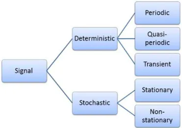
of observations of a variable over time. Each one of the aforementioned signals can be whether deterministic or stochastic, depending on its probabilistic character.

Determinis-tic signalsare those that might be described by mathematical functions and they can be

subdivided in periodic, quasi-periodic and transient. A signal isperiodicif it completes a

(30)

2. THEORETICALBACKGROUND 2.3. Methods of sensing biosignals

identical subsequent periods. Thus, consideringx(t)a periodic signal, it can be described as:

x(t) =x(t+kT) (2.1)

wherekis an integer.

The quasi-periodic group is the most common type and it refers to signals that present some similarity to a periodic function but do not meet the strict definition. A transient signal usually presents high-amplitude and short-duration. As examples, a sine wave is the perfect example of a periodic signal, an Electrocardiography (ECG) exam is the quasi-periodic representative and, a cell response illustrates the third class.

On the other hand, astochastic signalcan be defined as a statistical phenomenon that

evolves in time according to probabilistic laws and can be divided into stationary, if its probability distribution does not change when shifted in space or time, or non-stationary categories. As examples, brain alpha waves represent a stationary time series while an Electroencephalography (EEG) exam illustrates the second referred label. These relation-ships are exhibited on figure2.6.

Figure 2.6: Signal classification

2.3 Methods of sensing biosignals

In this section, only the activity recognition’s biosignals used in this project will be ad-dressed:EMG,GONandACC.

2.3.1 EMG

The human skeletal muscle is formed by cylindrical individual cells (named fibers) joined together by connective tissue.

(31)

brain or spinal cord to skeletal muscles. In order to reach the muscle, each axon (or ner-vous fiber) suffers ramifications and enervations into manifold muscle individual fibers. Although one motor neuron may innervate several muscle fibers, each fiber is innervated by only one motor neuron. A motor unit can be defined as a group of muscle fibres and their innervating terminal branches of one fibre whose cell body is located in the anterior horn of the spinal gray matter. Thus, when a neuron is activated, all of its enervated fibers respond to the impulse which causes its own electric signal and, consequently, leads to contraction. Although the electric impulse created and conducted by each fiber is too low (less than100mV), when several fibers transport the impulse simultaneously, they form

sufficient voltage that can be detected on the surface of the skin by a pair of electrodes. The detection, amplification and recording of these potential differences produced by the contraction of the skeletal muscle is calledEMG.

In this research, theEMGis obtained according to a non-invasive method, by placing the electrodes on the skin, as can be seen in2.7.

Figure 2.7: EMG acquisition, with an electrode placed on the skin, and example of a raw signal [5]

FromEMG’s analysis, it is possible to detect clinical abnormalities, level of activation, recruitment order or to evaluate movement biomechanics.

2.3.2 GON

In Medicine, GON is a method directly related to measure and document initial and subsequent joint’s angles.

A goniometer is a device used to quantify joint angles. Figure2.8shows the goniome-ter sensor used in this work from Biometrics Ldt1_{. This device is designed to measure}

rotations in two planes. When applied to the knee, the goniometer is capable to detect flexion/extension and valgus/varus. In this work, this sensor was used to measure the angle of the knee joint over time.

(32)

The maximum available angle range is defined as the Range of Motion (ROM) al-lowed at a joint and it is usually measured by the number of degrees from the starting to the ending position of a segment considering its full range of movement [13].

Figure 2.8: The figure represents two goniometers from Biometrics Ldt.

2.3.3 ACC

The ACC is a common procedure for kinematic and motion analysis. Motion can be quantified with an accelerometer which measures acceleration relative to itself. Hence, the signal from accelerometers may be used as motion detectors [14] or recognition [15] as well as for body-position and posture sensing [16]. A triaxial accelerometer is a sensor capable to estimate the value of acceleration along the x,y and z axes; it measures acceler-ation relative to free fall as well as its magnitude and direction, as a vector quantity. The output can be used to sense position, for example. In the context of this work, each one of the accelerometers presented the coordinate system shown in figure2.9.

Figure 2.9: Accelerometer axis representation and acquired signals [6]. This pictures also shows the sensors’ length (L), width (W) and height (H).

According to the figure, the acquired signals present positive, negative or neutral volt-age values which correspond, respectively, to a positive, negative or neutral proportional acceleration.

(33)

2. THEORETICALBACKGROUND 2.4. Biosignal pattern recognition and Classification

that, at rest, the sensor with its sensitive axis pointing towards the center of the Earth present1gas result, which concerns to gravity.

2.4 Biosignal pattern recognition and Classification

Biosignal pattern recognition concerns a group of measures applicable in biomedical signal processing. This phase involves all the stages from data acquisition to identifica-tion of the pattern and its usage for classificaidentifica-tion, detecidentifica-tion or parameter estimaidentifica-tion of the input value and machine’s comprehension of previous results or concepts obtained from feature extraction, feature selection, clustering and classification, detection or parameter estimation, which is important for learning [17].

Classificationis the allocation of a label to an input value: assuming known the num-ber of possible labels in a given data, the aim is to establish a rule whereby we can clas-sify new examples into one of the existing classes (Supervised Learning) which can be accomplished, depending on the problem, by different types of algorithms: logic-based, perceptron-based, instance-based or statistical algorithms [18]. On the contrary, Unsuper-vised Learning or Clustering occurs when the aim is to discover the existence of classes or clusters in a given set of observations, without a priori labelling.

Figure 2.10: Classification theory scheme

Figure2.10represents a classification scheme of a statistical learning algorithm: given a samplex, the classifier “reads” its characteristics and assigns it to a class. As

super-vised learning, each sample has a respective label,Y, which is already known. The X

represents a sample withX =X1, . . . , X_N whereN is the number of acquired channels.

After features extraction, each sample has a group of attributes,F = F1, . . . , FM where M is the number of features.

So the classification is well accomplished, the classifier needs to calculate p(Y|X)

which is the probability of the class is Y knowing that the sample is X. To do it, it

also determinesp(X|Y), the probability of the sample isX knowing that the class isY.

Ideally, the recognizer output,_Yˇ_{,is equal to}_Y_.

(34)

2. THEORETICALBACKGROUND 2.4. Biosignal pattern recognition and Classification

instance, i.e, is the percentage of well classified data in the testing data set.

Accuracy or Recognition Rate= Number of correct classifications

All tested cases (2.2)

However, this can also be expressed in terms of the errors

Error Rate= Number of wrong classifications

All tested cases (2.3)

Nevertheless, the correct error value is never known since it is impossible to test the classifier with all possible examples. Even so, for limited data, one possible technique is the leave-one-out cross-validation.Cross-validationis an evaluation method that involves

partitioning the initial data into complementary subsets , performing the analysis on one subset, thetrain set, and validating the analysis on the other subset, thetest setorvalidation set. When the validation set has only one sample and the remaining data is used for

training, the method is calledleave-one-out cross-validation[19].

2.4.1 Hidden Markov Models (HMM)

Hidden Markov Models (HMM) are a very powerful tool that statistically models a pro-cess that varies in time [20]. They are stochastic methods that use temporal information to model a sequence of observations. They are organized in a finite set of states, each of which is associated with a probability distribution, generally multidimensional. Tran-sitions among the states are defined by a set of transition probabilities. Each state has

probability function associated; thus, each state can generate an observation. However, the same sequences of observations can be achieved from different probabilities and from sequences of different states. A model can be described by Equation2.4,

λ={A, B,Π}={ai,j, bi, πi}, i, j= 1, . . . , N (2.4)

where:

• A={ai,j}is the transitions probability matrix between stateiandj(andN the

num-ber of states);

• B={bi}represents the matrix of all emission probabilities of the statei. Considering

a continuous distribution, this matrix refers to a probability density function;

• Π={πi} represents the matrix with the probabilities of a model being initialized

from the statei.

Given the form ofHMM, there are three items to consider so the model is useful in real applications. These points are the following:

(35)

2. THEORETICALBACKGROUND 2.5. State of the Art

2. Computation of the probability for the observation sequence, given the model;

3. Resolution of the most likely sequence of states that best explains the observations;

Figure2.11illustrates a simpleHMMwith a left-to-right topology.

Figure 2.11: HMM model with left-to-right topology with three emissors states [7]

The main goal is to determine the sequence of states that maximizes the posterior probability. To do that, theViterbi algorithm[20] is applied: computes the most likely state

sequence for time step. This algorithm is responsible for finding theViterbi path (most

likely sequence of hidden states) in a sequence of observed events.

2.5 State of the Art

Activity recognition concerns the automatic identification of types of physical activity from a set of measurements which can contain data from devices such video cameras, pedometers, heart rate monitors, accelerometers, EDA sensors, goniometers,EMG sen-sors, among others. Although activity recognition can be easily achieved by humans, in order to program it, automatic classification needs to improve itself considering classes and accuracy. Even so, the advantages are still relevant mainly because direct classifi-cation of visual data is expensive, very time-consuming and depends on the subjects as well as the recording environment.

The constant pursuit of electrophysiologic knowledge led to various experiments or studies in which several techniques and models were developed. In this section are pre-sented and discussed some of these studies, which results or limitations can be used as a start point for new research, structured by themes: work on gait, activity analysis and recognition as well as classification methods.

The intuitive procedure to evaluate human motion comes from the direct observation of movement which can be obtained from video camera data analysis. In [21], Boesnach et al. present a new procedure to model human motion based on 3Djoint features

(36)

2. THEORETICALBACKGROUND 2.5. State of the Art

pouring water from a coffepot into the cup and stirring the water in the cup with a coffee spoon. The extracted features were used to feed the artificial neural network. The results obtained were compared to those obtained fromHMMclassifier.

Gait analysis as well as posture are the primers subjects to investigate in health do-main [22–24]. Gait analysis studies involves continuous curves of data measured over a gait cycle [25]. In order to deliver a proper report, health technicians need to compare the exam results with statistical proved normal data. In [25] several tools to process statistical gait data are described.

Once the basic human movement is detected and modelled, different approaches can be applied to analyse different activities. Some studies present different methods or appli-cations onACCsignals, always keeping in mind the goal of activity classification with health purpose. For example, Takeda et al. in [26] exhibits a model possibility based on accelerometers and gyroscopes implemented in a suit so the human activity can be properly measured. Foerster et al. [27] uses a small number of calibrated piezoresistive accelerometers devices to validate the accelerometric evaluation against behaviour obser-vation and conclude about reliability. He proves that wearable accelerometers placed in different parts of the body identify correctly different postures and motions, by compar-ing the different behaviours and the respective kinematic analysis. In a similar approach, Moe-Nilssen et al. [28] reports a study on a portable system to measure gait parameters which are extracted from a triaxial accelerometer positioned in the lower trunk, during walking. In [29] the use of triaxial accelerometers successfully distinguished between activity (transitions sit-to-stand and stand-to-sit and walk) and rest. In the context of physical activity recognition, in [30], sedentary activities such as sitting or sleeping are discriminated from moderate intensity activities such as walking through the analysis of acceleration data.

ConcerningEMG, its analysis is useful for evaluation of muscle activation [31], whether for isolate muscles [32,33] or joint muscular groups [34]. The use ofEMGor electrogo-niometers have been applied mostly on kinematics evaluation [23,35] or on pattern com-parisons for diagnosis [36]. Recently, Fleicher et al. [37] prove the importance of muscular activity by presenting a method to determine the joints intended motions throughEMG analysis. After the motion is calculated, a leg orthosis can be real-time controlled to sus-tain patients in daily activities such walking or climbing stairs.

(37)

3

Acquisition

This chapter exposes the data acquisition procedure used in this work. Along the differ-ent sections, all the acquisition set up is explained: subjects, sensors and protocol.

3.1 Subjects

This work required the participation of one group of volunteer subjects. We performed a study with 6 male subjects. All participants were students and had no known disease related to gait or their knee. Table3.1 gives anthropometric characteristics on the par-ticipants. During the acquisition, all subjects wore shorts and sports shoes. Although the orthosis was not adapted to the anatomy of the subjects, all participants were able to move their knee freely and did not feel any pain. All subjects were shaved on the knee area to increase the quality of theEMGsignal and the electrodes’ adherence on the skin.

Subject’s Statistics

Height (cm) 181.33±8.16

Weight (kg) 78.17±10.32

Length of femur (cm) 46.17±6.18

Length of tibia (cm) 45.17±2.71

(38)

3. ACQUISITION 3.2. Material and Equipment

3.2 Material and Equipment

3.2.1 Orthosis

This project intends to investigate the possibility to classify isolated human activities from biosignal sensors integrated into a knee orthosis. We created a makeshift intelligent device by equipping a standard Ortema1 _{ipomax passive orthosis with sensors. Figure} 3.1illustrates the original equipment.

Figure 3.1: Standard right knee Ortema ipomax passive orthosis

The orthosis itself consists of two rigid shells, one for the upper and one for the lower part of the leg which are fixed to the leg with straps. The shells are connected by a joint on each side in order to allow flexion of the knee joint.

3.2.2 Sensor Layout and Signal Recording

In this research, we equipped the standard orthosis with sensors from PLUX-Wireless Biosignals2_{: two triaxial accelerometers (}_xyzPlux_{) and one goniometer. Additionally, six} EMGsensors (emgPlux) to measure muscle activity were put on the skin under the

ortho-sis.

Since all sensors should be integratable into the the orthosis in the future, our setup re-quires to place all sensors on or under the orthosis.

The orthosis with the full sensor setup can be seen in figure3.2.

A more detailed description about each sensor layout will be described on the next sections.

3.2.2.1 EMG

Concerning the surfaceEMG, and according to what was referred in chapter2, we wanted to acquire signal from six different muscles:vastus lateralis,vastus medialis,semitendinosus,

(39)

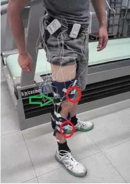
Figure 3.2: Complete experimental setup: two Bioplux research devices, twoACC(red circles), sixEMGand oneGONsensors (green arrow) placed on a regular Ortema right knee orthosis

semimembranosusand both parts of thegastrocnemius. Hence, sixEMGsensors were used

on these muscles, under the orthosis. Twelve surface electrodes were placed directly on the skin to acquire muscular activity; plus, the reference electrode was placed on the in-ternal part of the knee, with low percentage of muscles fibres. Figure3.3 illustrates the placement of the surface electrodes.

(40)

3.2.2.2 GON

One characteristic of a joint is its angular movement. The goniometer has the ability to capture the range of motion over time. However, the crucial aim of its use in this work is related to the angle measurement of the joint during different activities. The goniometer was placed on the joint so it can measure the angle of the orthosis joint which can be assume equal to the angle of the knee joint. Although the goniometer is biaxial only the information from the axis aligned to the degree of freedom of the knee joint was used. Figure3.4shows the sensor itself and this scenario.

(41)

3.2.2.3 ACC

The knee joint is basically made up of four bones: the largest thigh bone,femur, is at-tached by ligaments and capsule to thetibia; the fibula, that is located next to the tibia and runs parallel to it and, thepatella (or knee cap), that moves along with the knee. Figure3.5shows knee’s bone structure.

Figure 3.5: Principal bones of the knee joint [8]

The movements of the knee involve directly the femur and the tibia that are recruited by muscular contraction and tendon response. We used one triaxial accelerometer for each bone. Considering the accelerometers location, we put them vertically aligned with the patella, with the positivey axis pointing to the floor, placed on the frontside of the

orthosis, one on the lower part and other on the upper part to measure the acceleration of the tibia and the femur respectively (Figure3.6).

(42)

3. ACQUISITION 3.3. Acquisition Protocol

3.2.2.4 Recording devices

To record the data from our subjects, we used two bioPLUXresearch connected by the synchronism toolkit.

The bioPLUXresearch (figure3.7) is a device that collects and digitalizes signals from the sensors, transmitting them via bluetooth to the computer where the signals are shown in real-time. It has eight 12-bit analogue channels, with a sample frequency of1000Hz.

It also has a digital port, a connector for the transformer to recharge the internal battery and a channel to connect the reference electrode, an essential requirement to correctly monitor the electromyographic signal.

Figure 3.7: bioPLUXresearch system

In total we used fourteen of the sixteen available channels for our recording proce-dure. However, since one of the goniometer channels does not provide relevant informa-tion, we deleted it; so, at the end, we resorted thirteen channels.

3.3 Acquisition Protocol

The signal acquisition protocol was performed by all of the subjects.

The acquisition protocol is composed by a set of 8 activities, described in the following items, where an activity is considered as a sequence of movements.

(43)

3. ACQUISITION 3.3. Acquisition Protocol

• Activity 2. Sit and stand: The activity 2 consisted of one recording per subject where the participant, starting in a lower position, got up and sat down consecu-tively until 20 repetitions;

• Activity 3. Sit, stand and walk a few steps: Starting in a lower position, each participant was requested to get up and walk a few steps; here, five recordings per subjects were collected;

• Activity 4. Walk to a chair, turn, sit and stand: Each volunteer had to walk to a chair, turn, sit and stand consecutively until 20 repetitions. We also acquire one single recording per subject;

• Activity 5. Walk and stairs up: Each volunteer was asked to walk and walk stairs up a group of steps. In total, we collected ten recordings for each subject;

• Activity 6. Walk and stairs down: Each volunteer was asked to walk and walk stairs down a group of steps. In total, we collected ten recordings for each subject;

• Activity 7. Ascend a hill: We acquired two recordings of about two minutes each where each volunteer was requested to ascend a hill. The treadmill used as a ’hill’ was positioned with 27% of inclination;

• Activity 8. Descend a hill: Similar to activity 7, here the participants descended a hill during approximately two minutes for each one of the two recordings. The treadmill used as a ’hill’ was positioned with 27% of inclination.

(44)

(45)

4

Segmentation

In this chapter we intend to explain the segmentation procedure applied on the signals so that, at last, we can provide an overview about ourdata corpus. Therefore, we begin by

presenting some of the signals resulting from the acquisition.

4.1 Signal’s overview

In this section, we will exhibit an example of the raw data obtained directly from the ac-quisition.

As will be seen, each wave has its proper shape which can provide us different informa-tion about the moinforma-tion in acinforma-tion.

Considering theEMG, it is important to refer that the instance when muscular activity occurs depends on the function that muscle has; e.g, when flexors muscles show some contraction, extensors muscles tend to be approximately at rest and vice-versa.

On the other hand, theACCwave allow us to understand how and with which accelera-tion both lower limb’s segments move.

TheGONoutput show the evolution of knee’s angular position over time.

All of the biosignals’ acquisition procedure was accompanied by video recording to be used in future stages of this project.

As an example, the figures4.1,4.2and4.3represent theEMG,GONandACCsignals acquired for the activity 5,Walk and Walk stairs up, respectively.

4.2 Segmentation

(46)

4. SEGMENTATION 4.2. Segmentation

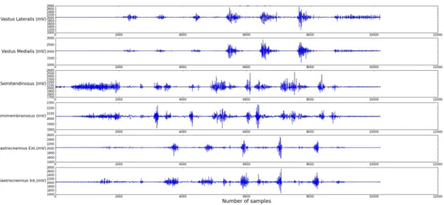
Figure 4.1:EMGraw signals for the sequence walk and walk stairs up. Plot shows quadri-ceps’, hamstrings’ and gastrocnemius’ activity, from top to bottom

Figure 4.2: GONraw signal for the sequence walk and walk stairs up. Plot shows how the range of motion evolutes over time for theyaxis

(47)

The purpose of the data segmentation step is to split the continuous sensor record-ings into motion primitives to be used as the classifier’s input. For the periodic motions

walk,stairs up,stairs down, andascendanddescenda hill, we define a motion primitive as

one complete gait cycle. For motions likestand-to-sitandsit-to-stand, we define a motion primitive as the movement that occurs between the two static postures “stand” and “sit”. We segment each continuous periodic signals in its unique motion primitives. We seg-ment automatically the periodic activities according to the standard segseg-mentation of gait cycles in [23,39,40].

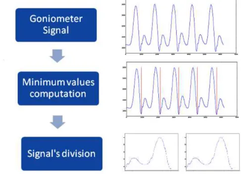
A gait cycle consists of a stance and a swing phase and starts and ends with the initial contact of the heel on the floor. At this point of the gait cycle the knee angle is minimal. Our automatic segmentation algorithm computes the local minima of the goniometer signal and takes these as segment borders. The signal is then split into motion primitives according to the found segment borders. Figure4.4illustrates this procedure.

The non-periodic movementsstand-to-sitandsit-to-standare segmented manually.

Figure 4.4: Representative scheme for the automatic segmentation algorithm. The signals refer to the movementwalk

We additionally checked the results of the automatic segmentation manually to verify the correctness of our data segmentation.

The figures4.5 and4.6 show our segmentation results for the activity 5, previously shown.

4.2.1 Data Corpus

(48)

Figure 4.5: One cycle for walking based on the analysis of the goniometer output Changed with the DEMO VERSION of CAD-KAS PDF-Editor (http://www.cadkas.com).Changed with the DEMO VERSION of CAD-KAS PDF-Editor (http://www.cadkas.com).Changed with the DEMO VERSION of CAD-KAS PDF-Editor (http://www.cadkas.com).

Figure 4.6: One cycle for walking stairs up based on the analysis of the goniometer output

anddescend. Table4.1shows the original database’s structure.

The database is unbalanced because the acquisition was not performed equally for each label. For example, for ascend anddescend, we recorded two times 2min of

walk-ing which lead to a much higher number of cycles than the activities which were not performed on the treadmill, e.g. climbing stairs. Our classifier computes themaximum a

posteriori probabilitywhich is a method used to obtain predictions on the most probables

hypothesis. Hence, the classifier’s input should have the same amount of information per each class. In order to get a balanced dataset for the evaluation we randomly chose 17 motion primitives per person for each activity, which is the minimum number of sam-ples we recorded over all activities. The resulting balanced data corpus therefore consists of 714 motion primitives. Table4.2shows the operational database’s structure.

(49)

Movements Number of isolated cycles

Walk 1356

Sit-to-stand 121

Stand-to-sit 116

Stairs up 170

Stairs down 172

Ascend 902

Descend 1021

Total 3858

Table 4.1: Number of isolated cycles from all subjects for each movement from all original acquired data

Movements Number of isolated cycles

Walk 102

Sit-to-stand 102

Stand-to-sit 102

Stairs up 102

Stairs down 102

Ascend 102

Descend 102

Total 714

(50)

(51)

5

Classification using

Hidden-Markov-Models

HMM

This chapter presents an overview about theHMMdecoding used in this work. During the exposition, we will outline the differences between the standardHMMand the ap-plied decoding procedure. Section5.1summarizes the classification procedure applied on this project.

5.1 Classification and Feature Extraction

We used continuous densityHMM as classifier [20]. Since HMMs can model stochas-tic processes over time, they are well suited to model signals that have a characterisstochas-tic temporal pattern, which is typically true for human motions. For each motion primi-tive we use anHMMwith a left-to-right topology with 10 states and a Gaussian Mixture Model (GMM) with two components. We apply four iterations of Expectation Maximiza-tion (EM) training in each of the experiments. As aforementioned, we used the BioKit toolbox developed at the Cognitive Systems Lab for the training and decoding.

For feature extraction the signal is windowed using a rectangular window function with 50ms window length and no window overlap. All features are computed on the resulting windows. We denote the samples in one window by(x1, . . . , x_N) whereN is

(52)

5. CLASSIFICATION USINGHIDDEN-MARKOV-MODELSHMM 5.2. BioKit

• Average

avg= 1 N

N−1

X

k=0

xk (5.1)

• Root mean square (RMS)

RM S =

r x2

1+x 2

2+. . .+x 2

N

N (5.2)

We therefore get a one-dimensional feature vector for the goniometer signal and six-dimensional feature vectors for the six accelerometer channels as well as the six EMG channels. We use feature fusion, also known as early fusion, to fuse the different signal modalities. Depending on the signal type, the features are computed and then combined in one feature vector by concatenation. Feature fusion is an appropriate fusion scheme if the underlying processes that produce the signals are synchronized. This can be assumed in our case because the underlying process, moving the knee, is the same for all signal modalities. Additionally, since all modalities were recorded synchronous with the same sampling rate, we consider this fusion scheme to be a reasonable choice.

The experiments and results are presented and discussed on section6.1.

5.2 BioKit

In this work, we used theBioKittoolbox which is a software from Cognitive Systems Lab

that performs theHMManalysis.

Given a sequence of observations, the BioKit converts them into feature vectors and stores them in different data structures.

After the conversion, theHMMis initialized: definition of the number of states, num-ber of gaussians, dimensionality and models’ list. Each model (oratom) refers to the most

primitive unit of which more complex models can be built; for example, in speech recog-nition, atoms are phonems. Atokenis created from atoms; for example, words (groups of letters). In this work, movements are the most basic unit we can get; so, tokens are atoms. Thus, each motion primitive is one atom which is described by one model. Considering this fact, it it possible to model arbitrary sequences of motion primitives.

The left-to-rightHMMtopology in use presents a mixture model defined.A mixture model is a way to represent the emission probability distribution. In this project, we usedGMM. In other words, GMM is a combination of Normal distributions to model more complex distributions; the more components it has, the more complex distributions it can model.

According to a standard procedure, the Viterbi path would be computed for each model. However, if we work with a large space this calculation becomes complex and time con-suming. Thus, the BioKit introduces the concept of Beam Searchwhich deletes the less

(53)

5. CLASSIFICATION USINGHIDDEN-MARKOV-MODELSHMM 5.2. BioKit

be seen as one possible path during the search. In short words, the beam search prune the hypothesis.

Furthermore, this software uses by default diagonal covariance matrices instead of full covariance matrices which decreases the number of parameters to train.GMMs are a combination of multidimensional normal distributions. A normal distribution is defined by mean and variance, and in the multidimensional case by the mean vector and the covariance matrix. To limit the number of parameters that need to be estimated, diagonal covariances matrices are used.

As an additional BioKit’s feature, it is possible to define agrammar(possible sequences

of atoms), which also helps on eliminating non-interesting paths.

(54)

(55)

6

Experiments

The goal of this chapter is lodge to the reader the experiments investigated and the results from our recognizer as well as their discussion (section6.2).

6.1 Experiments and Results

The main goal of this project is to investigate how well movement primitives can be correctly recognized. Since we are working with three different types of signals, our in-tention is to evaluate how much the different signal’s modalities contribute to the overall performance of the classifier. Hence, we explore all possible combinations of the different signals:EMG,GON,ACC,EMG&GON,GON&ACC,EMG&ACCandEMG&GON&ACC, whether in a context of subject’s dependency or independency. After the extraction of the features referred in5.1, in total, we work with 6, 1, 6, 7, 7, 12 and 13-dimensional features spaces, respectively. Each experiment was repeated four times.

For each different context, we compute the accuracy (see section2.4) of the respective leave-one-out cross-validation (see section2.4).

6.1.1 Experiment 1: Subject’s dependent context

The first test procedure investigates how the recognizer performs in a subject’s depen-dent context.

(56)

6. EXPERIMENTS 6.1. Experiments and Results

Signals’ Combination Classification Accuracy (%)

EMG 65.41±0.17

GON 83.33±0.12

ACC 97.34±0.01

EMG&GON 72.13±0.17

GON&ACC 98.32±0.05

EMG&ACC 81.23±0.14

EMG&GON&ACC 87.54±0.13

Table 6.1: Classification accuracy (mean and standard deviation) per combination of sig-nals in a subject’s dependent case

To evaluate the subject-dependent accuracy of the classifier we performed a leave-one-out cross-validation for each subjects data. We chose a set of 119 motion primitives avail-able for each subject. Figure6.1and table6.1shows a breakdown of the results for each of the signals’ combination.

EMG GON ACC EMG&GON GON&ACC EMG&ACC All 40 60 80 100 Accuracy (%) Signals

Figure 6.1: Classification accuracy per combination of signals in a subject’s dependent case

Based on these results, the recognizer accomplished its task with an accuracy between 65 and 98% with an average accuracy of 84%. We can also conclude that the combination of GON&ACC presents the highest classification accuracy. Since these signals present a more defined shape and consequently, a more defined pattern, this result could be expected. Likewise, theEMGpresents the lower accuracy.

The confusion matrices for each combination are represented on tables6.2to6.8.

Walk Stand-to-sit Sit-to-stand Stairs up Stairs down Ascend Descend

Walk 26 0 6 17 3 21 27

Stand-to-sit 1 95 4 0 0 0 0

Sit-to-stand 3 4 90 2 1 0 0

Stairs up 9 0 1 46 8 12 25

Stairs down 6 0 4 10 53 8 20

Ascend 3 0 8 8 2 67 13

Descend 7 0 0 6 2 5 80

(57)

Walk 89 0 0 2 0 0 9

Stand-to-sit 0 99 0 0 1 0 0

Sit-to-stand 0 0 96 2 1 1 0

Stairs up 1 0 0 73 16 2 9

Stairs down 0 0 0 3 92 0 5

Ascend 14 0 0 9 2 62 14

Descend 8 0 0 0 18 2 73

Table 6.3: Confusion matrix forGONset in a subject-dependent context (in percentage)

Walk 90 0 0 3 6 0 1

Stand-to-sit 0 100 0 0 0 0 0

Sit-to-stand 0 0 100 0 0 0 0

Stairs up 0 0 0 98 0 0 2

Stairs down 0 0 0 1 97 0 2

Ascend 0 0 0 1 1 98 0

Descend 0 0 0 2 0 0 98

Table 6.4: Confusion matrix forACCset in a subject-dependent context (in percentage)

Walk 43 0 0 8 9 16 25

Stand-to-sit 1 98 1 0 0 0 0

Sit-to-stand 1 1 97 0 1 0 0

Stairs up 5 0 0 55 6 10 25

Stairs down 3 10 1 0 55 10 22

Ascend 2 0 2 10 2 74 11

Descend 4 0 0 7 1 5 83

Table 6.5: Confusion matrix forEMG&GONset in a subject-dependent context (in per-centage)

Walk 95 0 0 0 3 1 1

Stand-to-sit 0 100 0 0 0 0 0

Sit-to-stand 0 1 99 0 0 0 0

Stairs up 0 0 0 98 2 0 0

Stairs down 0 0 0 0 98 0 2

Ascend 0 0 0 1 0 99 0

Descend 0 0 0 0 1 0 99

(58)

Walk 56 0 0 15 5 10 15

Stand-to-sit 1 98 0 0 1 0 0

Sit-to-stand 2 1 94 2 1 0 0

Stairs up 2 0 0 77 6 11 4

Stairs down 7 0 0 3 75 2 13

Ascend 6 0 0 10 1 82 2

Descend 7 0 0 1 4 2 86

Table 6.7: Confusion matrix forEMG&ACCset in a subject-dependent context (in per-centage)

Walk 75 0 0 8 7 3 7

Stand-to-sit 1 98 1 0 0 0 0

Sit-to-stand 1 1 95 2 1 0 0

Stairs up 2 0 0 83 7 8 0

Stairs down 2 0 0 5 82 1 10

Ascend 3 0 0 7 1 89 0

Descend 7 0 0 0 2 2 89

Table 6.8: Confusion matrix forEMG&GON&ACCset in a subject-dependent context (in percentage)

Each confusion matrix present how well the classifier performed in each activity type. Concerning the worst classified set, by analysing the table6.2, we may infer that only 26% from all of the walkprimitives are recognized correctly; 27% is labelled asdescend, 21%

as ascend, 17% asstairs up, 6% as sit-to-stand and the remaining 3% asstairs down.

Ad-ditionally, for the best performing combination (table6.6), we achieve high classification accuracies for all classes. As a further analysis, figure6.2and table6.9shows the classifi-cation accuracy per subject for the best performing combination.

1 2 3 4 5 6

90 95 100

Accuracy (%)

Subjects

Figure 6.2: Classification accuracy per subjects forGON&ACCset in a subject’s depen-dent case

(59)

Subjects Classification Accuracy (%)

1 97.32±0.04

2 99.11±0.02

3 97.32±0.04

4 98.22±0.03

5 98.22±0.03

6 99.11±0.04

Table 6.9: Classification accuracy (mean and standard deviation) per subject for GON&ACCset in a subject’s dependent case

Signals’ Combination Classification Accuracy (%) EMG 44.57±13.87

GON 61.46±11.67

ACC 75.05±22.65

EMG&GON 47.94±14.60

GON&ACC 78.70±21.64

EMG&ACC 55.52±14.46

EMG&GON&ACC 63.66±17.14

Table 6.10: Classification accuracy (mean and standard deviation) per combination of signals in a subject’s independent case

6.1.2 Experiment 2: Subject’s independent context

The second test procedure investigates how the recognizer performs in a subject’s inde-pendent context.

Subject’s independent context is when we train the recognizer with a database formed by data of all subjects except the one we intend to evaluate and test only with data of that test subject.

We evaluate the subject-independent performance with a leave-one-out cross-validation on the subjects. We use all samples in our database, resulting in 595 samples for training and 119 samples for testing for each subject. Figure6.3and table6.10presents the results for each of the signal’s combination.

EMG GON ACC EMG&GON GON&ACC EMG&ACC All 40 60 80 100 Accuracy (%) Signals

(60)

The recognizer performed with an accuracy between 44% and 79% with an average accuracy of 61%. We can also conclude that the combination GON&ACC exhibits the highest accuracy value, analogously to6.1.1. However, we can state that, compared to the subject-dependent case, the accuracy is much lower which can be explained by the variations in human motion for different subjects.

The confusion matrices for each signal’s combination are presented on tables6.11to 6.17.

Walk 5 0 2 31 6 50 7

Stand-to-sit 0 80 20 0 0 0 0

Sit-to-stand 0 19 57 0 3 19 3

Stairs up 1 0 1 41 21 10 26

Stairs down 0 0 5 15 50 17 13

Ascend 0 0 4 9 0 76 11

Descend 0 0 0 28 23 46 3

Table 6.11: Confusion matrix for EMGset in a subject-independent context (in percent-age)

Walk 36 0 0 14 44 7 0

Stand-to-sit 0 98 2 0 0 0 0

Sit-to-stand 0 0 71 29 0 0 0

Stairs up 0 0 0 66 11 16 7

Stairs down 1 0 0 1 86 3 9

Ascend 2 0 0 6 10 72 11

Descend 1 0 0 0 79 17 3

Table 6.12: Confusion matrix forGONset in a subject-independent context (in percent-age)

Walk 74 0 0 1 0 3 22

Stand-to-sit 0 83 0 3 0 0 14

Sit-to-stand 12 0 83 1 0 0 4

Stairs up 1 0 0 90 2 5 2

Stairs down 2 0 0 13 56 5 23

Ascend 28 0 0 5 0 67 0

Descend 17 0 0 0 14 0 70

Table 6.13: Confusion matrix forACCset in a subject-independent context (in percentage)

For the worst performing combination (table 6.11), the movement descend is easily

confused. From all of its primitives, only 3% are correctly recognized; 46% of them is labelled as ascend, 28% asstairs upand 23% asstairs down. Concerning theGON&ACC

set, the classesstairs downandascendare those with higher percentage of misclassification being confused withdescend andstairs up, respectively. This is not surprising since the

(61)

Walk 14 0 7 14 8 48 10

Stand-to-sit 0 80 20 0 0 0 0

Sit-to-stand 0 10 66 0 9 5 11

Stairs up 0 0 1 52 17 25 5

Stairs down 0 0 5 16 48 14 17

Ascend 1 0 5 12 0 70 13

Descend 7 0 0 12 29 46 6

Table 6.14: Confusion matrix for EMG&GONset in a subject-independent context (in percentage)

Walk 89 0 0 0 4 0 7

Stand-to-sit 0 83 0 0 17 0 0

Sit-to-stand 0 0 83 17 0 0 0

Stairs up 0 0 0 92 4 4 0

Stairs down 4 1 1 9 66 1 18

Ascend 1 0 0 32 0 67 0

Descend 19 0 0 0 9 0 72

Table 6.15: Confusion matrix for GON&ACC set in a subject-independent context (in percentage)

Walk 39 0 6 22 6 25 3

Stand-to-sit 0 89 0 0 11 0 0

Sit-to-stand 10 4 74 4 0 7 2

Stairs up 4 0 0 61 11 24 0

Stairs down 4 0 4 14 52 12 14

Ascend 17 0 3 16 0 57 8

Descend 29 0 0 6 28 19 18

Table 6.16: Confusion matrix for EMG&ACC set in a subject-independent context (in percentage)

Walk 60 0 5 14 7 9 5

Stand-to-sit 0 88 0 0 12 0 0

Sit-to-stand 0 1 77 6 0 16 0

Stairs up 1 0 0 66 11 23 0

Stairs down 4 0 0 13 55 13 15

Ascend 13 0 0 19 4 65 0

Descend 20 0 0 2 22 18 38

Human Activity Recognition for an Intelligent Knee Orthosis

Diliana Maria Barradas Rebelo dos Santos