Leonardo Sousa Gomes Marinho
Soluções Caóticas em um Problema de Programação Dinâmica
Este trabalho é dedicado a meu pai,
Agradecimentos
A realização desta dissertação de mestrado não teria sido possível sem o apoio de várias pessoas às quais sou muito grato.
Inicio agradecendo, em especial, ao meu orientador Daniel Cajueiro pelo apoio e paciência. Aos colegas da Universidade de Brasília pelas discussões e ajuda, em especial a Guilherme Solino pela valiosa ajuda na formatação do texto final. A Oona Rodrigues pelo apoio emocional, sem o qual esta tarefa teria sido muito mais árdua e menos prazerosa. Aos colegas do Banco Central do Brasil pelas dicas e frutíferas discussões.
Gostaria de agradecer também a Frederico Macedo e Alberto Mendes pela revisão do texto e sugestões de melhoria e aos funcionários da secretaria e membros da Comissão de Pós-Graduação do Departamento de Economia da UnB pela paciência com meus prazos incovenientes.
Também agradeço a meus sócios e amigos Pedro Vinícius, Guilherme Lavoratti e Rodolfo Carvalho pela paciência com minhas ausências em nossos compromissos num momento crucial de nossas vidas.
Resumo
Programação dinâmica é uma técnica onipresente em toda a ciência econômica, e é de interesse saber se as soluções para esta classe de problemas podem ser caóticas. A literatura na área provém, principalmente, do estudo de modelos de crescimento endógeno, mas o presente trabalho analisa um modelo proveniente da área de pesquisa conhecida como dinâmica humana, um ramo da teoria dos sistemas complexos. Um aspecto crucial da possibilidade de soluções caóticas para este tipo de problema é o valor do fator de desconto, onde a literatura econômica sugere que tais soluções só seriam comuns para fatores de desconto baixos, atípicos em economia. Aqui, para valores elevados do fator de desconto, são apresentadas soluções caóticas nos valores esperados de um modelo estocástico de programação dinâmica onde o espaço de estados é discreto. Tais soluções são analisadas numericamente por meio de gráficos e simulações e algumas de suas principais características, especialmente sua natureza caótica, são demonstradas analiticamente.
Abstract
Dynamic programming is a ubiquitous technique throughout economics, and it is of interest to know whether solutions to this class of problems may be chaotic. Literature in this area comes mainly from the study of endogenous growth models, but the present work analyzes a model from the research area known as human dynamics, a branch of complex systems theory. A crucial aspect of the possibility of chaotic solutions to this kind of problem is the discount factor value, where economic literature suggests that such solutions are common only for low, atypical values. Here, chaotic solutions for high values of the discount factor are presented for the expected values of a stochastic dynamic programming model with discrete state space. Such solutions are analyzed numerically and graphically through simulations and some of their main characteristics, especially their chaotic nature, are demonstrated analytically.
Lista de ilustrações
Figura 1 – PlanexL−xHshowing regions A, B and C.. . . 34
Figura 2 – Time evolution and cobweb diagram for equation (3.9) withk= 0. . . 36
Figura 3 – Time evolution and cobweb diagram for equation (3.9) withk= 0.3. . . 36
Figura 4 – Time evolution and cobweb diagram for equation (3.9) withk= 0.17911111111111111. 37 Figura 5 – Time evolution of (3.9) showing trajectories starting at 29.5 and 29.51. . . 38
Figura 6 – Cobweb diagrams for equation (3.10). . . 38
Figura 7 – Time evolution and cobweb diagram for equation (3.10). . . 39
Figura 8 – Time evolution of (3.10) showing trajectories starting at 29 and 29.00001. . . 40
Figura 9 – Time evolution and cobweb diagram for equation (3.10). Escaping trajectories. . . 40
Figura 10 – Time evolution and cobweb diagram for equation (3.11). . . 41
Figura 11 – Time evolution and cobweb diagram for equation (3.11). Oscillating sink.. . . 41
Figura 12 – Time evolution and cobweb diagram for equation (3.11). Chaos frontier. . . 42
Figura 13 – Bifurcation diagram for (3.11).. . . 43
Figura 14 – Time evolution and cobweb diagram for equation (3.11). Unstable periodic orbit. . . . 43
Figura 15 – Time evolution and cobweb diagram for equation (3.11). Chaos and floating point. . . 44
Figura 16 – Time evolution of (3.11) showing trajectories starting at 29.4 and 29.40001. . . 44
Figura 17 – Cobweb diagrams for equations (4.3) and (4.4).. . . 50
Figura 18 – Time evolution and cobweb diagrams for equation (4.3). . . 50
Lista de tabelas
Sumário
Introdução . . . 19
1 REVISÃO DA LITERATURA. . . 23
2 THE MODEL . . . 27
3 PROTOCOLS . . . 33
3.1 Introduction . . . 33
3.2 The Constant Protocol . . . 35
3.3 The Positive Slope Protocol . . . 37
3.4 The Negative Slope Protocol. . . 39
3.5 Conclusion . . . 45
4 CHAOS . . . 47
4.1 Some Properties of One-dimensional Maps . . . 47
4.2 Analysis of the Positive Slope Map . . . 48
4.3 Analysis of the Negative Slope Map . . . 49
5 CONCLUSÃO . . . 55
19
Introdução
Compreender o comportamento de pessoas individualmente ou coletivamente é de suma importância para ramos do conhecimento como a sociologia, a psicologia e a economia. Diversas abordagens são utilizadas em diferentes disciplinas, com ênfase em variados aspectos do comportamento humano, dependendo dos objetivos da pesquisa na área. Em particular, embora a ciência econômica tenha abordado o processo de tomada de decisão individual ou coletiva principalmente com base no presuposto da racionalidade dos agentes econômicos, recentemente este pressuposto tem sido relaxado de diversas formas, numa tentativa de explicar dados que não se encaixam na premissa do agente racional.
Uma destas abordagens com potencial para explicar determinadas características do compor-tamento humano de interesse para a Ciência Econômica é o ramo do conhecimento conhecido como dinâmica humana. Este é um ramo de pesquisa da teoria de sistemas complexos que tenta compreender o comportamento humano em interação com outras pessoas e diversos tipos de ambientes, frequente-mente utilizando-se perspectivas inspiradas em técnicas do ramo da física conhecido como mecânica estatística. Neste ramo existem modelos de filas e estudos sobre o comportamento de multidões, e um dos princiais trabalhos nesta área, principalmente por sua influência nas pesquisas realizadas posteriormente, é o artigo pioneiro deBarabasi(2005):The origin of bursts and heavy tails in human dynamics.
Neste trabalho, o autor modela o tempo de espera entre ações humanas utilizando um modelo de filas, na tentativa de explicar as “caudas gordas” observadas experimentalmente em processos deste tipo. Por exemplo,Paxson e Floyd(1995) abordam o problema do tráfego de informações em redes de computadores, focando em processos de acesso à rede iniciados por usuários, um típico problema de execução aleatória de uma determinada tarefa ao longo do tempo. Os autores concluem que o uso de processos de Poisson para a modelagem de tais processos mostra-se inadequado.
Tradicionalmente, a modelagem de eventos que ocorrem aleatoriamente ao longo do tempo é feita com processos de Poisson. Esta é uma escolha natural, dado que é a solução para este tipo de problema quando os eventos são estatisticamente independentes ao longo do tempo (veja, por exemplo,Daley e Vere-Jones(2003)). Porém, em várias situações reais, especialmente as que envolvem agentes humanos, esta suposição não é válida. Por exemplo: pessoas que chegam aos caixas de um supermercado observam o tamanho das filas e normalmente escolhem a menor, de modo que a probabilidade de chegada em uma fila específica é influenciada pelo tamanho desta fila em relação às outras.
Barabasi(2005) aborda o problema assumindo que pessoas tomam decisões de execução de tarefas organizadas em filas por meio de um protocolo que executa primeiro as tarefas com alta prioridade, deixando as tarefas com baixa prioridade esperando um tempo mais longo na fila. Com esta simples hipótese, ele mostra numericamente que a distribuição do tempo de espera entre a execução de tarefas segue uma lei de potência, com uma cauda muito mais gorda que a esperada num processo de Poisson. Posteriormente,Vazquez(2005) demonstrou analiticamente tais resultados.
Este modelo levou a um aumento da atividade de pesquisa na área, com diversas extensões da ideia original. Evidência experimental desta abordagem para várias atividades de execução de tarefas por pessoas é dada emVázquez et al.(2006). Outras contribuições são dadas por Hidalgo(2006),
20 Introdução
Numa abordagem alternativa,Cajueiro e Maldonado(2008) analisam a suposição de que as pessoas realizam tarefas por meio de um protocolo que preferencialmente executa a tarefa de maior prioridade primeiro. Porém, neste trabalho, a associação de prioridades às tarefas é feita de modo a minimizar um índice de custo dependente do estado do sistema. No modelo dos autores há duas filas (que podem ser vistas como apenas uma fila), uma com tarefas de alta prioridade e outra com tarefas de baixa prioridade. Em cada instante de tempo, o agente avalia o custo do estado atual, que é função do comprimento das filas, e também considera a dinâmica futura do sistema e os custos associados. Deste modo, os autores modelam tal situação por meio de um modelo estocástico de programação dinâmica com taxa de desconto intertemporal, onde a escolha do agente é aquela que minimixa o custo total, dado pelo custo atual e pelos custos esperados futuros descontados.
Uma das conclusões dos autores é que o protocolo utilizado depende da função custo encarada pelo agente. Esta função determina, em cada instante de tempo, o custo de manter uma tarefa em determinada fila por mais um período. Se a função custo é linear, executar a tarefa de alta prioridade é sempre ótimo, o que leva ao protocolo estudado emBarabasi(2005) entre outros. Porém, se o custo é quadrático, diferentes tipos de protocolo são possíveis. Dependendo do comprimento relativo das filas, pode ser ótimo em determinado instante executar apenas as tarefas de alta prioridade ou apenas as de baixa prioridade. Há também a possibilidade de indiferença em relação a qual das tarefas executar. Finalmente, ao final do artigo eles ainda mostram que, dependendo dos parâmetros do sistema, o protocolo considerado pode gerar uma dinâmica complexa.
Esta possibilidade de dinâmica complexa é interessante porque mesmo com valores elevados do fator de desconto ela pode ocorrer. Cabe ressaltar que, mesmo não sendo estritamente caótica no sentido matemático do termo, para quase todos (no sentido de Lebesgue) os valores de parâmetros, a dinâmica do sistema é aperiódica. Tal resultado vai de encontro a alguns resultados na literatura que sugerem que soluções caóticas em problemas de programação dinâmica tenderiam a ocorrer apenas com fatores de desconto baixos, característica esta não muito comum em problemas econômicos. Portanto, uma conclusão apressada é que tais soluções caóticas não seriam de interesse econômico.
O presente trabalho é inteiramente baseado em Cajueiro e Maldonado(2008), sendo uma extensão do artigo dos autores. No trabalho original, a dinâmica complexa encontrada não é caótica no sentido utilizado emLi e Yorke(1975), que é uma definição de caos muito aceita na literatura de sistemas dinâmicos. Aqui, diferentes protocolos que também são soluções ótimas do problema de programação dinâmica são considerados, e são apresentados dois protocolos ótimos que induzem soluções caóticas para o comportamento esperado do sistema. Tais protocolos exploram a região do espaço de estados onde o agente mostra-se indiferente às opções de alta ou baixa prioridade.
No primeiro protocolo considerado, aqui chamado de protocolo com inclinação positiva, devido ao fato de o mapa que define tal protocolo ter uma inclinação positiva na região de indiferença, as tarefas são realizadas de modo a aumentar as chances de o sistema ir em direção à fronteira entre a região de indiferença e uma das regiões onde é ótimo realizar a tarefa de alta ou baixa prioridade. Por exemplo: se o sistema se encontra na região de baixa prioridade, as tarefas de baixa prioridade são executadas até o tamanho das filas atingir a região de indiferença. Uma vez nesta região, as tarefas da fila de alta prioridade são executadas com probabilidade positiva, de modo a trazer o sistema de volta à região anterior, e a probabilidade de execução da tarefa de alta prioridade aumenta à medida que o sistema entra mais profundamente na região de indiferença, tornando cada vez mais provável que as filas voltem à região de baixa prioridade. Uma situação parecida ocorre se o sistema iniciar na região de alta prioridade.
21
abordagem numérica do mapa com inclinação positiva, onde suas propriedades, especialmente sua natureza caótica, são analisados de maneira informal por meio de gráficos e simulações. Já na Seção
4.2, este protocolo é analisado de maneira mais formal, e seu comportamento caótico é demonstrado e analisado matematicamente.
O segundo protocolo considerado é uma espécie de imagem espelhada do primeiro, e é chamado de protocolo com inclinação negativa. Como o nome sugere, o mapa que o define tem inclinação negativa na região de indiferença. Seu comportamento é inverso ao do protocolo com inclinação positiva. Por exemplo: estando o sistema na região de baixa prioridade, ao atingir a região de indiferença, as tarefas de baixa prioridade ainda são preferencialmente executadas, com a probabilidade de execução das tarefas de alta prioridade tornando-se maior à medida em que o sistema adentra mais profundamente a região de indiferença. Então, finalmente alcança-se o ponto, dependente dos parâmetros, em que as tarefas de alta prioridade são executadas com probabilidade 1, fazendo o sistema retornar à região de indiferença e finalmente atingir a região de baixa prioridade novamente, gerando uma alternância entre as regiões de alta e baixa prioridade.
Como será demonstrado nas Seções 3.4 e 4.3, este mapa apresenta um comportamento bastante complexo, com regiões do espaço de parâmetros onde a dinâmica é completamente caótica, e outras regiões onde a dinâmica é periódica. Na Seção3.4, a análise é feita de maneira mais informal, por meio de gráficos e simulações. Finalmente, na Seção4.3a análise do protocolo com inclinação negativa é feita de maneira mais formal, com demonstrações matemáticas de sua natureza caótica e com a explicação do que ocorre nas fronteiras onde o sistema deixa de ser caótico e passa a se comportar de maneira periódica.
23
1 Revisão da Literatura
Como já mencionado na Introdução, o trabalho pioneiro feito emBarabasi(2005),The origin of bursts and heavy tails in human dynamics, levou a um aumento na atividade de pesquisa na área. Enquanto o citado autor modelava a realização de tarefas ao longo do tempo por pessoas supondo que estas realizam primeiro tarefas de alta prioridade, conseguindo replicar as “caudas gordas” observadas experimentalmente neste tipo de processo, outros autores extenderam tal abordagem em diferentes direções.
Estudos sobre a temporalidade da realização de tarefas por pessoas foram feitos em variados contextos.Henderson e Bhatti (2001) investigam o acesso de jogadores em redes de jogoson-line.
Wang e Guo(2010) analisam tais conceitos no contexto de operações logísticas, enquantoDezsö et al.
(2006) concentram-se em acessos a determinadas páginas na internet. Outros trabalhos relacionados sãoGonçalves e Ramasco(2008) eGao et al.(2013).
Trabalhos empíricos sobre correspondências escritas que observam escalas de tempo que vão de alguns meses a vários anos podem ser encontrados emEckmann, Moses e Sergi(2004),Wu et al.
(2010),Oliveira e Barabási(2005),Qu, Wang e Wang(2011),Malmgren et al.(2008),Malmgren et al.
(2009) eFormentin et al.(2014). Estes estudos estão relacionados a outros onde “caudas gordas” são encontradas em atividades realizadas por pessoas ou animais:Hanai et al.(2006),Crane, Schweitzer e Sornette(2010),Proekt et al.(2012),Jung et al.(2014) eMryglod et al.(2015).
Diversas tentativas de explicar estas “caudas gordas”, tipicamente modeladas por distribuições com caudas que obedecem a uma lei de potência foram feitas. O já mencionado trabalho pioneiro de
Barabasi(2005) é um exemplo.Hidalgo(2006) mostra analiticamente e numericamente que “caudas gordas” podem surgir no processo de realização de tarefas ao longo do tempo em nível populacional se os indivíduos que compõem a população realizam as tarefas individualmente como num processo de Poisson com tempos característicos distintos. O fenômeno também é observado se os agentes variam suas taxas de realização de tarefas de maneira determinística ou estocástica.
Grinstein e Linsker(2006) deduzem analiticamente resultados assintóticos para modelos es-tocásticos de filas com tarefas executadas de acordo com uma associação de prioridades contínua.
Masuda, Kim e Kahng(2009) encontram analiticamente valores para o expoente das caudas de distri-buições de atividades realizadas ao longo do tempo. EmWalraevens et al.(2012), os autores aplicam técnicas da teoria de filas, como o modelo de prioridades estocástico para analisar tempos de espera. Outros trabalhos na área são:Blanchard e Hongler(2007),Min, Goh e Kim(2009),Cho et al.(2010),
Kim e Chae(2010),Jo, Pan e Kaski(2012),Jiang et al.(2013) eFormentin et al.(2015).
O artigo mais importante relacionado ao presente trabalho éCajueiro e Maldonado (2008). Como já mencionado na Introdução, aqui é feita uma extensão do trabalho dos autores. Porém, o foco da extensão está concentrado nas consequências dinâmicas do processo de minimização de custos utilizado no artigo, ao invés da distribuição das tarefas realizadas pelo agente ao longo do tempo, que é o pricipal foco dos trabalhos mencionados anteriormente na presente seção. Especificamente, o ponto focado aqui é a solução do problema de programação dinâmica apresentado emCajueiro e Maldonado
(2008).
24 Capítulo 1. Revisão da Literatura
em vários ramos da ciência econômica. Um ponto de interesse é saber se as soluções deste tipo de problema são “bem comportadas”.
Com os avanços ocorridos na teoria dos sistemas dinâmicos a partir da década de 1960, especi-almente com o melhor entendimento do fenômeno do caos, o interesse nas propriedades das soluções de problemas de programação dinâmica ressurgiu, especialmente na literatura sobre crescimento agregado, onde pretendia-se investigar se flutuações no crescimento econômico poderiam ser causadas por fatores endógenos e não por choques externos.
Boldrin e Montrucchio(1986) mostram que, para fatores de desconto suficientemente baixos, a função que determina a política ótima para problemas de crescimento ótimo pode ser de qualquer tipo, podendo inclusive apresentar comportamento caótico.Montrucchio e Sorger(1996) mostram um resultado que poderia ser interpretado como o recíproco do primeiro: eles provam que para gerar soluções ótimas com grande entropia topológica nesta classe de modelos, o fator de desconto deve ser pequeno.
Porém, apesar da importância do resultado dos autores, um valor alto da entropia topológica é uma condiçãosuficiente, porém, não énecessáriapara a ocorrência de caos na definição adotada porLi e Yorke(1975). Corroborando este fato,Nishimura, Sorger e Yano(1994) mostram que é possível encontrar infinitos modelos como os considerados por Montrucchio e Sorger (1996) que possuem políticas ótimas exibindo caos ergódico. Mitra e Sorger (1999) mostram que caos topológico é um fenômeno robusto neste tipo de problema mesmo para valores do fator de desconto arbitrariamente elevados. Eles encontram restrições exatas para o fator de desconto sob as quais o mapa logístico e o “mapa da tenda” (tent map), dois bem conhecidos mapas caóticos, podem ser políticas ótimas de modelos de crescimento agregado. Entretanto, nestes casos os valores encontrados pelos autores são pequenos comparados aos tipicamente encontrados em problemas econômicos.
Boldrin et al.(2001) estudam um modelo de crescimento endógeno que apresenta soluções caóticas. Outros trabalhos sobre caos em problemas econômicos que envolvem programação dinâmica sãoGardini, Sushko e Naimzada(2008), Gardini et al.(2009),Fanti e Gori (2011) eGupta, Stander et al.(2014), por exemplo. Uma coleção de artigos relacionando problemas de otimização e caos é apresentada emMajumdar, Mitra e Nishimura(2000).
As raízes da teoria do caos remontam a Poincaré (Poincaré(1890)) ainda no século XIX, num estudo sobre o problema dos três corpos na mecânica celeste (Diacu e Holmes(1996)). Estudos sobre equações diferenciais não-lineares foram realizados por diversos autores. Alguns trabalhos importantes na área sãoBirkhoff(1927),Kolmogorov(1941),Kolmogorov(1979),Cartwright(1949) eSmale(2000). Apesar destas observações feitas na primeira metade do século XX, demorou até que ficasse evidente para a comunidade científica que modelos lineares não poderiam explicar diversos fenômenos que aparentavam ser aleatórios mas eram na verdade determinísticos, como o famoso mapa logístico e várias observações experimentais vindas principalmente da física. Com o surgimento dos computadores, a teoria ganhou fôlego, já que passou a ser possível simular diversos sistemas com grande velocidade e precisão. Isso levou ao trabalho pioneiro do meteorologista Edward Lorenz (Lorenz(1963)), que concluiu que mesmo com um modelo detalhado da atmosfera não seria possível prever o tempo para períodos muito longos adequadamente.
25
equações diferenciais como por seu interesse intrínseco.
Mapas envolvem a iteração de uma função, operação que se mostra importante desde os tempos babilônicos, onde estes utilizavam tal operação na construção de um calendário preciso. A partir do século XVIII, outra importante aplicação de mapas surgiu com os métodos de determinar numericamente os zeros de uma função, como o método de Newton-Raphson. Porém, foi apenas no início do século XX que a análise sistemática deste tipo de operação começou a ser feita, com os trabalhos de Julia e Fatou. Aplicações da teoria de mapas na análise de sistemas de maior dimensão são feitas emGuckenheimer
(1976),Collet, Eckmann e Koch(1981),Levi(1981) eHolmes e Whitley(1984).
De particular interesse para o presente trabalho são os mapas unidimensionais, onde uma refererência que compila grande diversidade de resultados importantes é Melo e Strien (2012). Os mapas estudados na presente dissertação também são da classe de mapas lineares por pedaços, e uma referência no assunto éBernardo et al.(2008).
27
2 The Model
The model is the same as inCajueiro e Maldonado(2008). Their model has two queues: a high priority queue(H)and a low priority queue(L) with sizesxH andxL, respectively. The state of the
system at timetis given by(xL(t), xH(t)), and the cost of this state is given byg(xL(t), xH(t)). This cost
function has the following property:
∂g(xL, xH)
∂xL x
L=xH
<∂g(xL, xH) ∂xH
x
L=xH
(2.1) which means that the marginal cost for an additional task arriving atLis smaller than if the task arrives at H, for equally sized queues. For this reason, they callH a high priority queue andLa low priority queue.
At each discrete time step, a task arrives atH with probabilityλρor atLwith probabilityλ(1−ρ). At the same time step, first task inH is executed with probabilityµu(xL(t), xH(t))or first task inLis
executed with probabilityµ[1−u(xL(t), xH(t))], whereu(xL, xH)is a state dependent control function.
This control function is chosen in order to minimize the total cost function:
Ju(xL, xH) =Eu " ∞
X
t=0
αtg(xL(t), xH(t))
xL, xH #
(2.2)
whereEu[·|xL, xH]is the expected value conditioned on initial state(xL, xH) = (xL(0), xH(0))and control
functionu. Parameterαis the discount factor.
The following quadratic form for the cost function is explicitly assumed:
g(xL, xH) =hLx2L+hHx2H, 0< hL< hH. (2.3)
Here, the same approach to minimize (2.2) throughuis followed. The principle of optimality
(Bertsekas et al.(1995)) togheter with the Banach fixed point theorem imply that the minimum cost functionminuJu(xL(t), xH(t))at timet, if it exists, is given by the solution to the Bellman equation:
J(xL(t), xH(t)) =
min
u
g(xL(t), xH(t)) +αEu[Ju(xL(t+ 1), xH(t+ 1))|xL(t), xH(t)] . (2.4)
To solve (2.4), first notice that the evolution of states is given by:
xL(t+ 1) =xL(t) +ǫL(t)−θL(t) (2.5a)
xH(t+ 1) =xH(t) +ǫH(t)−θH(t) (2.5b)
whereǫL(t)andǫH(t)model the arrival of tasks inLandH, respectivelly. Also,θL(t)andθH(t)model
the execution of tasks inLandH and their distributions are given by:
ǫL(t)∼Bernoulli(λ(1−ρ)) (2.6a)
ǫH(t)∼Bernoulli(λρ) (2.6b)
θL(t)∼Bernoulli(µ(1−u)) (2.6c)
28 Capítulo 2. The Model
Here,Bernoulli(p)is the Bernoulli distribution with parameterp1. Moreover, these variables arenot independent, because ifǫL(t) = 1thenǫH(t) = 0and vice versa. The same is true forθLandθH. Define
eL(t) =ǫL(t)−θL(t) (2.7a)
eH(t) =ǫH(t)−θH(t) (2.7b)
so that
xL(t+ 1) =xL(t) +eL(t) (2.8a)
xH(t+ 1) =xH(t) +eH(t). (2.8b)
In equations (2.7) or (2.8),eL(t)andeH(t)are alsonot independent. So, it is convenient to write
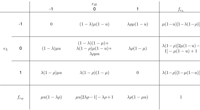
down their joint probability distribution as shown in Table1.
eH
-1 0 1 feL
-1 0 (1−λ)µ(1−u) λρµ(1−u) µ(1−u)[1−λ(1−ρ)]
eL 0 (1−λ)µu
(1−λ)(1−µ)+
λ(1−ρ)µ(1−u)+
λρµu
λρ(1−µ) λ(1−ρ)[2µ(1−u)− 1]−µ(1−u) + 1
1 λ(1−ρ)µu λ(1−ρ)(1−µ) 0 λ(1−ρ)[1−µ(1−u)]
feH µu(1−λρ) µu[2λρ−1]−λρ+ 1 λρ(1−µu) 1
Tabela 1 – Joint probability distribution ofeLandeH. Marginal distributions are also displayed.
Using Table1, equation (2.4) may be easily rewritten as equation(1)inCajueiro e Maldonado
(2008):
J(xL, xH) =F(xL, xH) + min
u u(xL, xH)G(xL, xH) (2.9)
1 x∼Bernoulli(p)ifx= 1with probabilitypand 0 with probability1−p. The Bernoulli density is given by:
px
(1−p)1−x
29
whereu=u(xL(t), xH(t))is the control function valued at state(xL, xH) = (xL(t), xH(t)). Also,
F(xL, xH) =g(xL, xH) +λρ(1−µ)αJ(xL, xH+ 1)
+λ(1−ρ)(1−µ)αJ(xL+ 1, xH)
+ (1−λ)µαJ(xL−1, xH)
+λρµαJ(xL−1, xH+ 1)
+λ(1−ρ)µαJ(xL, xH)
+ (1−λ)(1−µ)αJ(xL, xH)
(2.10)
and
G(xL, xH) = (1−λ)µα[J(xL, xH−1)−J(xL−1, xH)]
+λρµα[J(xL, xH)−J(xL−1, xH+ 1)]
+λ(1−ρ)µα[J(xL+ 1, xH−1)−J(xL, xH)]
(2.11)
To solve (2.9), the same reasoning presented inCajueiro e Maldonado(2008) is followed. This minimization problem is a linear programming, andu(xL, xH)explicitly depends on the signal ofG(xL, xH),
such that, ifG(xL, xH) <0, the maximum possibleu(xL, xH)minimizes (2.9), that is,u(xL, xH) = 1.
Similarly, ifG(xL, xH)>0,u(xL, xH) = 0. Finally, ifG(xL, xH) = 0, thanu(xL, xH)may be any value in
[0,1]. Notice that, given real constantsa, b, c, d, e, quadratic polynomials like
a+bxL+cxH+dx2L+ex
2
H (2.12)
equiped with sup-norm form a Banach space. So, becauseg(xL(t), xH(t))has the same structure (2.12)
(see (2.3)) for allt, it follows that the sequence of functions obtained by successive iterations of (2.9)
has the same functional form. Therefore, a polynomial as in (2.12) is the solution to (2.9). To determine the constantsa, b, c, d, e, substituteJ(xL, xH) =a+bxL+cxH+dx2L+ex2H into (2.9) and solve for the
constants.
IdentifyingG(xL, xH)>0,G(xL, xH) = 0andG(xL, xH)<0cases with subscripts A, B and C,
respectivelly, the substitution process for each case gives the following equations depending on the signal ofG:
Ji(xL, xH) =ai+bixL+cixH+dx2L+ex2H (2.13)
Gi(xL, xH) =µ{bi−ci+ 2(dxL−exH) +d[2λ(1−ρ)−1] +e(1−2λρ)} (2.14)
wherei=A, B, C. The constants in equations (2.13) and (2.14) are given by:
aA=
α
(1−α)3{[(1−α)(µ+ (1−ρ)λ)) + 2α(λ
2+µ2−µλ)+
+ 2ρλ(µ(1 +α) +λα(ρ−2))−2µλ]hL+λρ(1−α+ 2λρα)hH}
bA=
2αhL[−µ+λ(1−ρ)]
(1−α)2
cA=
2αhHλρ
(1−α)2
30 Capítulo 2. The Model
aB=
α
(hL+hH)(1−α)3
{[2λα(1−α)(−ρ2λ+ 2λρ−1−λ−ρ)]h2L+ + [δ(2λρα2+ 4λα−4λρα+ 1−2λ−2α+α2−2λα2+ 2λρ)+ + 2λ(−µα+ 2λρ2α2+ 2λρα−2λρ2α−α2µ−2λα2ρ+λα2)+ + 2µ(α−α2+µα2)]hLhH+ [δ(−4λρα+ 2δ−α2+ 2δα2+ 2λρα2−
−1−4αδ+ 2α+ 2λρ) + 2λρ(λρα2−λρα−α2+α)]h2
H}
bB=
1 (hL+hH)
h2
L
1−α[1−2λ(1−ρ)] + hLhH
(1−α)2[2α(λ−µ)+
+ (2λρ−1 + 2δ)(1−α)]
cB=
1 (hL+hH)
h2
H
1−α(1−2λρ−2δ) + hLhH
(1−α)2[2(λ−µα)− −(2λρ+ 1)(1−α)]
(2.16)
aC=
α
(1−α)3{[λ(1−α)(1−ρ) + 2λ
2α(1−ρ)2]h
L+
+ [(1−α)(µ+λρ) + 2µ2α+ 2λρ(λρα−µα−µ]hH}
bC=
2αhLλ(1−ρ)
(1−α)2
cC=
2αhH(−µ+λρ)
(1−α)2
(2.17)
d= hL 1−α e= hH
1−α
(2.18)
whereδ∈[δ, δ]is a parameter that defines the set of points such thatG(xL,(hL/hH)xL+δ) = 0, and the
linear relation betweenxLandxH inside the argument of this equation is obtained seting equation (2.14)
to zero. Parametersδandδare given by:
δ= 1 1−α
1−α
2 −λρ
+ hL
hH
−1−α
2 +λ(1−ρ)−αµ
(2.19a)
δ= 1 1−α
1−α
2 −λρ+αµ
+ hL
hH
−1−α
2 +λ(1−ρ)
. (2.19b)
It is easy to see that
δ→δ⇒JB(δ)→JAandGB(δ)→GA (2.20)
δ→δ⇒JB(δ)→JCandGB(δ)→GC (2.21)
31
xH=
hL
hH
xL+δ (2.22a)
xH=
hL
hH
xL+δ (2.22b)
arise, where for each region a suitable value foruminimizes2.9. In next chapter, this solution is explored
in more detail, and some possible choices for protocoluare analysed, including the possibility of chaotic
33
3 Protocols
3.1 Introduction
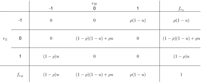
In this chapter, three different optimal protocols will be analyzed. From now on only the (long run) stationary caseµ=λwill be considered. If, additionally, it is assumedλ= 1, dynamics becomes completely one-dimensional. To see this, substituteλ=µ= 1in Table1. Results are shown in Table2.
Notice that the sumeL+eHequals zero anywhere probabilities are positive, implying the sum of (2.8a)
and (2.8b) to be constant for allt:
xL(t) +xH(t) =xL(0) +xH(0) =σ0 (3.1)
This equation is a downward slope straight line in(xL, xH)plane with -1 slope passing through
(xL(0), xH(0)), as Figure1shows.
eH
-1 0 1 feL
-1 0 0 ρ(1−u) ρ(1−u)
eL 0 0 (1−ρ)(1−u) +ρu 0 (1−ρ)(1−u) +ρu
1 (1−ρ)u 0 0 (1−ρ)u
feH (1−ρ)u (1−ρ)(1−u) +ρu ρ(1−u) 1
Tabela 2 – Joint probability distribution of eL and eH with λ = µ = 1. Marginal distributions are also
displayed.
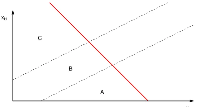
Figure1also shows regions A, B and C delimited by the straight lines:
xH=
hL
hH
xL+δ (3.2a)
xH=
hL
hH
xL+δ (3.2b)
where, as shown inCajueiro e Maldonado (2008) and Chapter 2, three regions arise with different regimes: in A,u= 0; in B,uis any functionu:B →[0,1]and in C,u= 1. Here,δandδare given by
equations (2.19).
Cajueiro e Maldonado(2008) analyzed the constant protocol functionu=ρ+k,k >0, and found that the expected valueEt[x(t+ 1)]follows a dynamics topologically conjugate to the translation in the
circle (seeMelo e Strien(2012)), which exhibits a complex behavior. Depending on system parameters, this behavior can be quite complicated, but its dynamics cannot be considered chaotic in the sense ofLi e Yorke(1975). However, other protocols are possible.
34 Capítulo 3. Protocols
C
B
A
x
Hx
LFigura 1 – PlanexL−xH showing regions A, B and C delimited by dashed lines and the solid straight
line, given by (3.1), where dynamics occurs.
The protocol proposed inCajueiro e Maldonado(2008) is given by:
u(x) =
0 ifx∈A
ρ+k ifx∈Bandk∈[−ρ,(1−ρ)] 1 ifx∈C
(3.3)
Two protocols that will be shown to exhibit chaotic behavior are given by the following equations:
u+(x) =
0 ifx∈A
minhmax1−k
xA x+k,0
,1i ifx∈Bandk>1
1 ifx∈C
(3.4)
u−(x) =
0 ifx∈A
minhmax k
xAx−k,0
,1i ifx∈B andk>0
1 ifx∈C
(3.5)
wherexA= hHhδ+hLσ0
H+hL is the point that separates regions A and B. These equations represent optimal
policies for (2.4) withλ=µ= 1given the cost function (2.3). The expected value ofxt+1may be written, for these protocols, as
Et[xt+1] =xt+ρ−u (3.6)
Et[xt+1] =xt+ρ−u+ (3.7)
3.2. The Constant Protocol 35
Substituting equations (3.3), (3.4) and (3.5) into equations (3.6), (3.7) and (3.8), respectively, leads to the following dynamic equations:
xt+1=
xt+ρ ifxt6xA
xt−k ifxA< xt< xCandk∈[−ρ,(1−ρ)]
xt+ρ−1 ifxt>xC
(3.9)
x+t+1=
x+t +ρ ifx+t 6xA
1 + k−1
xA
x+t +ρ−k ifxA< x+t < xB+andk>1
x+t +ρ−1 ifx+t >xB+
(3.10)
x− t+1=
x−
t +ρ ifx
− t 6xA
1− k xA
x−
t +ρ+k ifxA< x −
t < xB−andk>0
x−
t +ρ−1 ifx
− t >xB−
(3.11)
wherexB+=min
h k
k−1xA, xC
i
,xB−=min h
1 +1
k
xA, xC i
,xC=xA+1−ααandαis the discount factor.
For all these protocols there is a special parameterk. Basically,kcontrols the slope and location of the functionu:B →[0,1], which is linear in all cases considered. This parameter strongly influences
model dynamics. Notice that, depending on k, there are truncations at pointsxB+ andxB−. This is
becauseu∈[0,1], and if it goes outside this interval, it is set to the closer value in the interval, causing a
“degeneration” of policies inside region B. This makes policies in region B wherex > xB+orxB− equal
policies in regions A or C, depending on each case.
The dynamics of equations (3.9), (3.10) and (3.11) will be analysed in the following sections.
3.2 The Constant Protocol
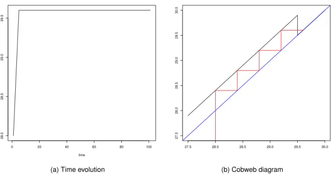
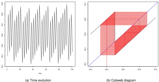
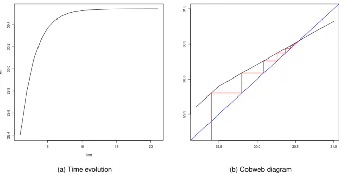
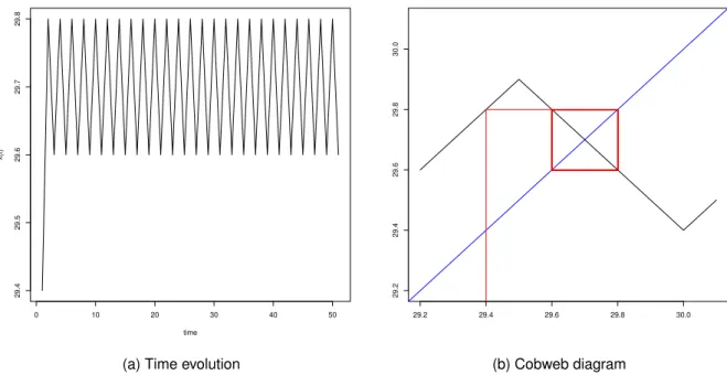
InCajueiro e Maldonado(2008), the authors considered protocol (3.3), which is constant over region B. If k = 0, each point in region B represents a fixed point. It is easy to see that if xt ∈ Aor
xt∈C, next iterates will soon or later reach region B and then the system stops there. Time evolution
and cobweb diagram for this situation are shown in Figure2.
Notice thatxvalues are increased arithmetically byρ= 0.4at each iteration in region A and
immediately stops after reaching region B atx= 29.6.
For positivekvalues, the behavior is more complicated. Actually, as observed inCajueiro e
Maldonado(2008), this dynamics is topologically conjugate to the translation in the circle (Melo e Strien
(2012)) and the system follows a limit cycle of periodp+qif ρk =pq is a irredutible ratio representation of
a rational number. Negativekvalues are symmetric to positive ones and dynamics is qualitatively the
same. As an example, consider ρ= 0.4andk = 0.3, whose irredutible ratio representation is ρk = 43.
These parameters imply a periodic motion with periodp+q= 7, and its dynamics is shown in Figure3.
If the ratioρ
k is irrational, the motion is quasi-periodic and never exactly repeats itself (Hilborn
(2000)). Since rational numbers have Lebesgue measure zero, its fair to say that the “typical” case is quasi-periodic. But, since rationals are also dense inR, and because computers have finite precision, it is impossible to “see” a really aperiodic trajectory through simulation. Figure4shows time evolution and cobweb diagram for equation3.9withρ= 0.4andk= 0.17911111111111111, which have a very large
36 Capítulo 3. Protocols
0 20 40 60 80 100
28.0 28.5 29.0 29.5 time x(t)
(a) Time evolution
27.5 28.0 28.5 29.0 29.5 30.0
27.5 28.0 28.5 29.0 29.5 30.0
(b) Cobweb diagram
Figura 2 – Time evolution and cobweb diagram for equation (3.9) with k = 0. Parameter values are
ρ= 0.4,α= 0.9,hL = 10,hH = 20,x0= 28andσ0= 99.
0 20 40 60 80 100
29.3 29.4 29.5 29.6 29.7 29.8 29.9 time x(t)
(a) Time evolution
29.2 29.4 29.6 29.8 30.0
29.2
29.4
29.6
29.8
30.0
(b) Cobweb diagram
Figura 3 – Time evolution and cobweb diagram for equation (3.9) withk= 0.3. Parameter values are
ρ= 0.4,α= 0.9,hL = 10,hH = 20,x0= 29.4andσ0= 99.
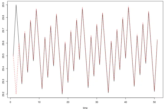
This dynamics has some complexity, but it is not chaotic in a mathematical sense. The model (3.9) lacks some properties that are associated with chaotic systems. This will be shown in next chapter. As an illustration, Figure5shows time evolution for two trajectories starting at close different points. The system lacks sensitive dependence on initial conditions. Yet, sensitive dependence on initial conditions is regarded as the main signature of chaos.
3.3. The Positive Slope Protocol 37
0 20 40 60 80 100
29.3 29.4 29.5 29.6 29.7 29.8 29.9 time x(t)
(a) Time evolution
29.2 29.4 29.6 29.8 30.0
29.2
29.4
29.6
29.8
30.0
(b) Cobweb diagram
Figura 4 – Time evolution and cobweb diagram for equation (3.9) with k = 0.17911111111111111.
Pa-rameter values areρ= 0.4,α= 0.9,hL = 10,hH = 20, x0 = 29.4andσ0 = 99. Period is 17,911,111,111,111,115.
this system. Using the equation
λ= 1
n
ln|f′
(x0)|+ln|f′(x1)|+· · ·+ln|f′(xn−1)|
(3.12) for the Lyapunov exponent of a trajectory(x0, x1, ..., xn−1), it is clear that this value and its average over any set of trajectories is zero for alln. So, this system does not have sensitive dependence on initial conditions. For details, seeHilborn(2000).
3.3 The Positive Slope Protocol
Protocol (3.4) has a negative slope in region B and leads to a positive slope along the same region for equation (3.10). This positive slope is greater than 1 ifk >1and, in this case, it is responsible
for a very complicated dynamics. Ifk= 1, dynamics in region B becomes the same as in region C and the system behaves like in Section3.2, with dynamics depending on the ratio ρ
1−ρ. So, only thek >1
case will be considered here.
Dynamic equation (3.10) is discontinuous atxAandxC. Discontinuous maps are more
compli-cated than continuous ones, but here the system is piecewise-linear, and the literature for this class of systems is relatively mature (see, e.g.,Bernardo et al.(2008)).
As in Section3.2, regions A and C have no fixed points and, once the system is in one of them, it is “pushed back” into region B. In this region there exists one fixed point, given by equation
x∗
=1 +k−1
xA
x∗
+ρ−k, whose solution isx∗
= k−ρ
k−1xA. An important fact about this fixed point is that
it is unstable, because the derivative of the map evaluated at it,1 + k−1
xA
, is greater than 1 (seeHilborn
38 Capítulo 3. Protocols
0 10 20 30 40 50
29.2
29.3
29.4
29.5
29.6
29.7
29.8
29.9
time
x(t)
Figura 5 – Time evolution of (3.9) showing trajectories starting at 29.5 (solid line) and 29.51 (dashed line). Both are very close to each other even after 50 iterations. Parameter values arek= 0.31,
ρ= 0.4,α= 0.9,hL = 10,hH = 20andσ0= 99. Period is 35.
29.0 29.5 30.0 30.5 31.0 31.5 32.0
29.0
29.5
30.0
30.5
31.0
31.5
32.0
(a) Cobweb diagram: AttractorA
32 34 36 38
32
34
36
38
(b) Cobweb diagram: AttractorC
Figura 6 – Cobweb diagrams for equation (3.10). In6a,x0= kk−−ρ1xA−0.1and in6b,x0=kk−−ρ1xA+ 0.1.
Parameter values arek= 10,ρ= 0.4,α= 0.9,hL= 10,hH= 20andσ0= 99.
3.4. The Negative Slope Protocol 39
attractorC. Trajectories converge to either attractor,AorB, depending on the signal ofx0−x∗. AttractorA has a very complicated dynamics, which will be shown to be chaotic. AttractorChas a periodic dynamics. Chaotic behavior of attractor Ais due to a greater than 1 slope of the map in region B. Notice that, becausek is not low enough, region B in attractorChas slope 1, leading to a periodic dynamics as described in Section3.2.
Figure7displays the chaotic nature of trajectories in attractorA. A comparison with Section3.2
plots shows how a greater than 1 slope leads to a more complicated behavior. Dynamics in Figure7
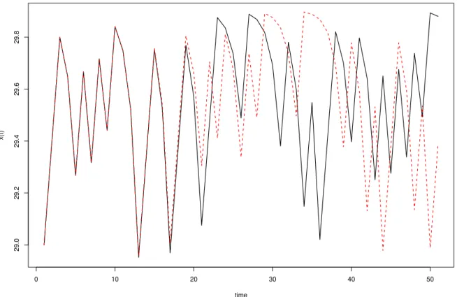
seems completely aperiodic. Also, it has sensitive dependence on initial conditions. Figure8shows two trajectories diverging after only 20 iterations even starting at points differing by only 0.00001.
0 20 40 60 80 100
29.0 29.2 29.4 29.6 29.8 time x(t)
(a) Time evolution
28.8 29.0 29.2 29.4 29.6 29.8 30.0
28.8 29.0 29.2 29.4 29.6 29.8 30.0
(b) Cobweb diagram
Figura 7 – Time evolution and cobweb diagram for equation (3.10). Parameter values arek= 45,ρ= 0.4,
α= 0.9,hL= 10,hH= 20,x0= 29andσ0= 99.
It is worth noting that, ifx∗
< xA+ρ, the fixed pointx∗falls “inside” the attractorAand, eventually,
trajectories will escape to attractorC. Figure9illustrates this situation. This happens because the attractor Ais chaotic. Moreover, every point within interval[xA+ρ−1, xA+ρ]can be arbitrarily approximated by
points in trajectories initiated at almost all (in Lebesgue sense) points of the basin of attraction ofA. So, pointsxnsuch thatx∗< xn6xA+ρwill be repelled to attractorC.
In Chapter4, a more formal analysis of the properties of map (3.10) is done.
3.4 The Negative Slope Protocol
Protocol (3.5) has a positive slope in region B and leads to a negative slope along the same region for equation (3.11) ifk > xA. If k = 0, dynamics in region B is the same as in region A, so
trajectories go to attractorCand the system behavior can be described as in Section3.2. Ifk >0, the
derivative of the map in region B is less than 1 and a fixed point given by x∗
= 1 +ρk
xAarises for
k>1−α
α ρxA. This fixed point has a derivative whose modulus is less than 1 if
1−α
α ρxA6k <2xA, leading
to a stable fixed point as shown in Figures10and Figure11. The emergence of this fixed point causes attractorCto collapse and not to be an attractor anymore.
40 Capítulo 3. Protocols
0 10 20 30 40 50
29.0
29.2
29.4
29.6
29.8
time
x(t)
Figura 8 – Time evolution of (3.10) showing trajectories starting at 29 (solid line) and 29.00001 (dashed line). Both start much closer than in Figure5, but here trajectories are completely different after only 20 iterations. Parameter values arek= 45,ρ= 0.4,α= 0.9,hL= 10,hH = 20and
σ0= 99.
0 20 40 60 80 100
30
32
34
36
38
time
x(t)
(a) Time evolution
29.0 29.5 30.0 30.5 31.0
29.0
29.5
30.0
30.5
31.0
(b) Cobweb diagram
Figura 9 – Time evolution and cobweb diagram for equation (3.10). Parameter values are k = 50,
ρ = 0.4, α = 0.9, hL = 10, hH = 20, x0 = 29 and σ0 = 99. These parameters imply
x∗
3.4. The Negative Slope Protocol 41
5 10 15 20
29.4 29.6 29.8 30.0 30.2 30.4 time x(t)
(a) Time evolution
29.5 30.0 30.5 31.0
29.5
30.0
30.5
31.0
(b) Cobweb diagram
Figura 10 – Time evolution and cobweb diagram for equation (3.11). Parameter values arek= 1−α α ρxA+
10< xA,ρ= 0.4,α= 0.9,hL= 10,hH = 20,x0= 29.4andσ0= 99.
0 10 20 30 40 50
29.4 29.5 29.6 29.7 29.8 time x(t)
(a) Time evolution
29.2 29.4 29.6 29.8 30.0
29.2
29.4
29.6
29.8
30.0
(b) Cobweb diagram
Figura 11 – Time evolution and cobweb diagram for equation (3.11). Parameter values arek= 1.9xA,
ρ= 0.4,α= 0.9,hL= 10,hH= 20,x0= 29.4andσ0= 99. Thiskvalue leads to a negative slope so that stable trajectories oscillates around the fixed point before converging.
region B, system oscillates in a period two orbit forever. Figure12shows this periodic behavior, which is a frontier between stable trajectories and chaos. Ifk >2xA, the slope of equation (3.11) in region B is
less than -1. So, the fixed pointx∗becomes unstable.
For2xA< k < nxA, wherenis an integer such that pn is the irreductible ratio representation ofρ,
trajectories are chaotic. Why this happens will be analysed in Chapter4. As an example, takeρ= 0.4
such thatρ=2
42 Capítulo 3. Protocols
0 10 20 30 40 50
29.4 29.5 29.6 29.7 29.8 time x(t)
(a) Time evolution
29.2 29.4 29.6 29.8 30.0
29.2
29.4
29.6
29.8
30.0
(b) Cobweb diagram
Figura 12 – Time evolution and cobweb diagram for equation (3.11). Parameter values arek = 2xA,
ρ= 0.4,α= 0.9,hL= 10,hH= 20,x0= 29.4andσ0= 99. Thiskvalue is a frontier between stable and chaotic regimes.
where two vertical lines atk = 2xA andk = 5xA highlight the chaotic region between them. Various
features of the dynamics can be seen in this figure, some of which will be more carefully analyzed in Chapter4. The main characteristics are the bifurcation points atk= 2xAandk=nxA. While the former
depends linearly onxA, the latter depends onρin a non-trivial manner. Actually, for almost allρvalues,n
does not exist and chaos can be found for arbitrarilly highkvalues. Moreover, as can be seen in Figure
13, fork > nxA there is a stable period 5 orbit for eachk which, by Sharkowskii’s theorem (Hilborn
(2000)), implies the existence of orbits of any period above 5 in the so called Sharkowskii ordering. In particular, there are chaotic orbits for allk > nxA. More on this fact will be discussed in Chapter4.
Another important feature is that, for this system, chaos is robust. That is to say, there are no stable periodic windows for2xA< k < nxA. Of course, there are infinite unstable periodic orbits for each
kvalue inside this interval (seeHilborn(2000)), and one such example is shown in Figure14fork= 3xA
andn= 5.
There are some interesting features about the period 4 orbit shown in Figure14. This orbit is given by29.37→29.77→29.57→29.97→29.37→..., and is easy to check that it is periodic. As will be shown
in Chapter4, it is unstable because the point 29.7 belongs to a region where the map has a less than -1 slope. Besides it being periodic, simulating too much points on a computer leads to an annomalous behavior due to a combination of floating point error and the inherent instability of the orbit, as can be seen in Figure15. This happens because the binary representation of the initial point 29.3 is not finite (actually, it is 11101.01001100110011...). So, the tiny floating point operations errors are amplified by this chaotic map, and the instability of the period 4 orbit becomes clear.
3.4. The Negative Slope Protocol 43
Figura 13 – Bifurcation diagram for (3.11). Vertical lines arek= 2xAandk= 5xA. Parameter values are
ρ= 0.4,α= 0.9,hL= 10,hH = 20andσ0= 99.
0 10 20 30 40 50
29.3
29.4
29.5
29.6
29.7
29.8
29.9
time
x(t)
(a) Time evolution
29.0 29.2 29.4 29.6 29.8
29.0
29.2
29.4
29.6
29.8
(b) Cobweb diagram
Figura 14 – Time evolution and cobweb diagram for equation (3.11). Parameter values arek = 3xA,
44 Capítulo 3. Protocols
0 100 200 300 400 500
29.3
29.4
29.5
29.6
29.7
29.8
29.9
time
x(t)
(a) Time evolution
29.0 29.2 29.4 29.6 29.8
29.0
29.2
29.4
29.6
29.8
(b) Cobweb diagram
Figura 15 – Time evolution and cobweb diagram for equation (3.11). Parameter values arek = 3xA,
ρ= 0.4,α= 0.9,hL = 10, hH = 20, x0 = 29.3and σ0 = 99. Deviations from the original period 4 orbit are caused by errors on computer floating point operations.
0 10 20 30 40 50
29.2
29.3
29.4
29.5
29.6
29.7
29.8
29.9
time
x(t)
Figura 16 – Time evolution of (3.11) showing trajectories starting at 29.4 (solid line) and 29.40001 (dashed line). Both start much closer than in Figure5and trajectories are completely different after only 20 iterations. Parameter values arek= 3xA+ 10,ρ= 0.4,α= 0.9,hL= 10,hH= 20
3.5. Conclusion 45
3.5 Conclusion
47
4 Chaos
4.1 Some Properties of One-dimensional Maps
In this chapter, the chaotic behavior of equations (3.10) and (3.11) is analyzed in more detail and some analytical results are presented. To achieve this purpose some concepts are necessary. Let
f:I→Ibe a one-dimensional map from some intervalI⊂Rto itself. Definition 1. A pointx∗
is afixed pointoff if it satisfiesx∗
=f(x∗
).
A fixed point is called asinkor anattracting fixed pointif points sufficiently close tox∗are
attracted tox∗. A fixed point is called asourceor arepelling fixed pointif points sufficiently close to
x∗
are repelled fromx∗. More precisely,
x∗is a sink if exists
ǫ >0such that ifx∈(x∗
−ǫ, x∗
+ǫ)\{x∗
}then
limk→∞f(k)(x) =x
∗. Similarly,
x∗is a source if exists
ǫ >0such that ifx∈(x∗
−ǫ, x∗
+ǫ)\{x∗
}then existsksuch thatf(k)(x)6∈(x∗
−ǫ, x∗
+ǫ). Here,f(k)(x)representsk-th iterate off starting atx. Next result is well known in dynamical systems literature.
Theorem 1. Letf be a smooth map onRandx∗
a fixed point off. If|f′
(x∗
)|<1, thenx∗
is a sink. If |f′
(x∗
)|>1, thenx∗
is a source.
Demonstração. SeeAlligood, Sauer e Yorke(1996).
Technically speaking, this result is valid wheref is differentiable, andf does not need to be
smooth on all its domain, as stated. But, if the trajectory contains points wheref is non-differentiable,
some care must be taken. One way to deal with this is to consider left and right derivatives, but calculations get more involved. Since for all maps considered here the non-differentiability points are finite and at most two, is simpler to consider only trajectories that do not contain these points. From now on, this assumption is implicit. Finally, here non-differentiable points have zero measure for all iterations of the map and, if they are included, conclusions are the same.
Another important observation concerns the stability of periodic orbits. Let(x0, x1, ..., xn−1)be a periodnorbit of the mapf. It is easy to see thatxi=f(n)(xi)for alli∈ {0,1, ..., n−1}. In other words,
the points of a periodnorbit are fixed points of the iterated mapf(n). Applying the chain rule tof(n)(x
i)
leads to the following equation:
(f(n))′
(xi) =f ′
(x0)f
′
(x1)· · ·f
′
(xn−1)∀i∈ {0,1, ..., n−1} (4.1)
Equation (4.1) shows that for every point of a periodic orbit,(f(n))′ has the same value, and this
value determines the stability of the orbit by Theorem1. So, the following corollary applies:
Corollary 1. The periodic orbit(x0, x1, ..., xn−1)is a sink if
|f′
(x0)f′(x1)· · ·f′(xn−1)|<1
and a source if
|f′
48 Capítulo 4. Chaos
Corollary1gives a simple criteria to determine the stability of a periodic orbit: If|f′
(x0)f′(x1)· · ·f′(xn−1)|<
1, then the orbit is a sink, and nearby trajectories are attracted to the periodic orbit(x0, x1, ..., xn−1). So, this orbit is stable. Otherwise, if|f′
(x0)f′(x1)· · ·f′(xn−1)|>1, then the orbit is a source, and nearby trajectories are reppeled from the periodic orbit(x0, x1, ..., xn−1). So, this orbit is unstable.
Finally, an important fact is that the only attractors that exist in non-circular one-dimensional maps of a interval are stable periodic orbits or chaotic attractors (seeBernardo et al.(2008) andMelo e Strien(2012)). Circular maps are those with a circular state space, like map (4.8), and they may show quasi-periodic motion.
4.2 Analysis of the Positive Slope Map
The positive slope map is given by equation (3.10), reproduced here for convenience:
xt+1=
xt+1+ρ ifxt6xA
1 +k−1
xA
xt+ρ−k ifxA< xt< xB andk>1
xt+ρ−1 ifxt>xB
(4.2)
wherexB =min h
k
k−1xA, xC i
,xA=hHδ+hLσ
0
hH+hL ,xC=xA+ α
1−α, andαis the discount factor.
The map is piecewise-linear and assumingk > 1, x∗
> xA+ρ, andx0 < x∗ the trajectory remains trapped on attractorA(see chapter3), which is chaotic according to the following proposition:
Proposition 1. The attractorAis chaotic for allk >1.
Demonstração. Letf be the map representing equation (4.2). ThatAis an attractor is a consequence of
x∗
> xA+ρ.
Supposingx0< x∗,x0is in the basin of attraction ofA, so trajectories starting atx0will remain inA. There are no fixed points insideA, so any trajectory have to pass through regions A and B. Actually, ifx0 ∈A, the trajectory is(x0, x0+ρ, x0+ 2ρ, ...)eventually reaching region B. Once in region B, the trajectory is pushed back to region A.
The map slope in region A is 1 and in region B it is1 +k−1
xA
>1, given thatk >1. Therefore,
for any long enough trajectory(x0, x1, x2, ..., xn),
|f′
(x0)f
′
(x1)· · ·f
′
(xn)|>1
because ifxi ∈A, thenf ′
(xi) = 1and, at least for onei,f ′
(xi) =
1 +k−1
xA
>1.
In particular, every periodic trajectory inA, if it exists, is unstable by corollary1. Given that the only attractors that exist in non-circular one-dimensional maps are stable periodic orbits or chaotic attractors, the result follows.
Proposition1shows that if trajectories are attracted toA, then dynamics is chaotic for allk >1
4.3. Analysis of the Negative Slope Map 49
4.3 Analysis of the Negative Slope Map
Besides being continuous, the map in equation (3.11) is more complicated. Its equation is reproduced here for convenience:
xt+1=
xt+ρ ifxt6xA
1− k xA
xt+ρ+k ifxA< xt< xBandk>0
xt+ρ−1 ifxt>xB
(4.3)
wherexB =min h
1 +1
k
xA, xC i
,xA = hHhδ+hLσ0
H+hL ,xC =xA+
α
1−α, andαis the discount factor. This
map is related to the following map:
xt+1=
xt+ρ ifxt6xA
xt+ρ−1 ifxt> xA
(4.4)
which is topologically equivalent to the translation in the circle, so as equation (3.9) (seeMelo e Strien
(2012)). Notice that map (4.4) is the limit fork→ ∞of map (4.3). But, even for finitek, both maps can
have equivalent dynamics. Suppose an orbit
(x0, x1, ...)such that,∀i∈ {0,1,2, ...},xi6∈(xA, xB). (4.5)
It is clear that this orbit is the same for maps (4.3) and (4.4), since only regions wherexi6xAorxi>xB
are visited, and in these regions both maps are the same. The existence of an orbit such as (4.5) can be estabilished by a simple example. Suppose the following parameter values for equations (4.3) and (4.4):
ρ= 0.4 (4.6a)
α= 0.9 (4.6b)
hL= 10 (4.6c)
hH= 20 (4.6d)
x0= 29.5 (4.6e)
σ0= 99 (4.6f)
Figure 17 shows cobweb diagrams for equations (4.3) and (4.4) with parameters given by equations (4.6) andk= 157.5for equation (4.3). Notice both period 5 trajectories given by same values
(29.5,29.9,29.3,29.7,29.1, ...). Also, Figure17suggests that, for sufficiently lowk, equation (4.3) cannot
“sustain” this period 5 trajectory, since one of its points will fall inside the interval(xA, xB). Actually, for
k= 137.5, equation (4.3) becomes chaotic, as exhibited in Figure18.
Suggestion given by Figure17is indeed true, and will be proved through some steps. First, notice that the equivalence of maps (4.3) and (4.4) for trajectories with property (4.5) permits analysis of such orbits by the translation in the circle map. As pointed out in chapter3, trajectories for map (4.4) are related toρrationality. If ρis rational and is represented by an irreductible ratio np, the motion is
periodic with periodn. Ifρis irrational, the motion is quasi-periodic. To see this, it is convenient to make
the change of variablesyt=xt−xA−ρ+ 1, such that the map (4.4) may be written as
yt+1=
yt+ρ ifyt61−ρ
yt+ρ−1 ifyt>1−ρ
50 Capítulo 4. Chaos
29.0 29.2 29.4 29.6 29.8
29.0
29.2
29.4
29.6
29.8
(a) Map (4.3)
29.0 29.2 29.4 29.6 29.8
29.0
29.2
29.4
29.6
29.8
(b) Map (4.4)
Figura 17 – Cobweb diagrams for equations (4.3) and (4.4). Parameter values are ρ = 0.4, α = 0.9,
hL= 10,hH= 20,x0= 29.5,σ0= 99and, for equation (4.3),k= 157.5. Both trajectories are exactly the same.
0 20 40 60 80 100
29.2
29.4
29.6
29.8
time
x(t)
(a) Time evolution
29.0 29.2 29.4 29.6 29.8
29.0
29.2
29.4
29.6
29.8
(b) Cobweb diagram
Figura 18 – Time evolution and cobweb diagrams for equation (4.3). Parameter values areρ = 0.4,
α= 0.9,hL= 10,hH = 20,x0= 29.5,σ0= 99, andk= 137.5.
which is a mapf: [0,1]→[0,1]from unit interval to itself. More conciselly:
yt+1=yt+ρmod 1 (4.8)
where mod 1 means to take only the fractionary part of the result.
4.3. Analysis of the Negative Slope Map 51
(4.8)ntimes leads to
yt+n =yt+nρmod 1 (4.9)
which leads to
yt+n=yt+n
p
n mod 1=yt (4.10)
that is to say that map f(n)fixes all points in[0,1]and any orbit(x
0, x1, ...) is a periodnorbit. If ρis irrational, orbits are dense in[0,1], and this result is known as Jacobi’s Theorem (seeDevaney(2003)).
One important fact here is: if(x0, x1, ..., xn−1)is a periodnorbit of map (4.7), then, for anyxiin
this orbit,xi+1n mod 1 also belongs to the orbit. This is the result of next lemma.
Lemma 1. Let(x0, x1, ..., xn−1)be a periodnorbit of map (4.8)and ρ= pn an irreductible fraction. If
xi∈ {x0, x1, ..., xn−1}, then exists an integermsuch thatf(m)(xi) =xi+1
n mod 1.
Demonstração. Sincef(m)(x
i) =xi+mnp mod 1, then the lemma afirms thatxi+mnp =xi+n1 mod 1
has a solution for integerm. Subtractingxileads tompn = n1 mod 1. This means that there is an integerr
such that
mp n =
1
n+r. (4.11)
Rearranging gives
mp−rn= 1. (4.12)
From number theory (seeShokranian, Soares e Godinho(1994)), this equation has a solution for integers
mandrif, and only if,pandnare coprime. But this is the case, since pn is irreductible.
Now, the main result of this section:
Proposition 2. Map (4.3) is chaotic for allk ∈ (2xA, nxA), where ρ = np is an irreductible fraction
representation.
Demonstração. Suppose k > 2xA. Thus, the unique fixed point x∗ = (1 + ρk)xA is unstable, since
|f′
(x∗
)|>1. Also,|f′
(x)|>1for allx∈(xA, xB). So, by Corollary1, all stable periodic orbits cannot have
points inside the interval(xA, xB). Since in this case map (4.3) behaves like map (4.8), these periodic
orbits have periodn, whereρ=np is a irreductible fraction representation.
Consider a periodnstable orbit(x0, x1, ..., xn−1)and takexi ∈S={x0, x1, ..., xn−1}such that
xi=max{x∈S;x6xA} (4.13)
Notice that exists at least onexj ∈S such thatxj >xB > xA. This fact togheter with Lemma1imply
xi+n1 ∈S. By equation (4.13),xi6xA< xi+1n. Also,xB= 1 +k1xA=xA+xkA. Supposek < nxA.
This impliesxB =xA+ xkA > xA+ 1n >xi+n1. So,xi+n1 ∈(xA, xB), which contradicts the stability
assumption for(x0, x1, ..., xn−1). Thus, ifk∈(2xA, nxA), there are not stable periodic orbits on map (4.3).
Since only attractors that exist in non-circular one-dimensional maps are stable periodic orbits or chaotic attractors, the result follows.
Proposition2supposes a rationalρ. Of course, ifρis irrational, orbits in map (4.7) are dense in
[0,1]and any trajectory will eventually reach interval(xA, xB), leading to chaos for allk >2xA.
Bifurcation diagram in Figure13shows the chaotic region delimited by vertical lines given by
52 Capítulo 4. Chaos
anything about what happens fork>nxA ifρis rational. Figure13suggests that only periodic orbits
remain, and indeed only period 5 orbits are visible on the graph.
As mentioned in section3.4, Sharkowskii’s theorem implies, fork>nxAand figure13orbits, the
existence of orbits of any period above 5 in the Sharkowskii ordering of the integers (seeMelo e Strien
(2012)).
Definition 2. The following ordering on the set of natural numbers is calledSharkowskii ordering:
3≺5≺7≺9≺11≺ · · · ≺2n+ 1· · · · · · ≺6≺10≺14≺ · · · ≺2(2n+ 1)· · · · · · ≺2m3≺2m5≺ · · · ≺2m(2n+ 1)· · · · · · ≺2n ≺2n−1≺2n−2≺ · · · ≺2≺1
So, in Figure13, Sharkowskii’s theorem guarantees the existence of chaotic orbits for allk>nxA
even for rationalρ. Why are they not visible in Figure13? Someone may be tempted to say that these
chaotic orbits are unstable, but this is meaningless, since chaotic orbits are unstable by definition. Certainly, period 5 orbits are stable, but why are they always reached in this example?
An important fact about Figure13is that it shows asymptoticbehavior of the orbits. Before converging to period 5 orbits, trajectories behave like chaotic ones for a dense set of initial values. One example of such transient behavior is shown in figure19.
This figure highlights an interesting property of map (4.3). Forkvalues slightly abovenxA, the
transient behavior is more persistent. This is due to fact that the region(xA, xB)is almostn1 in size. In
fact, for figure19parameters,xB−xA= 0.1998645<0.2 = 1n. The tiny differenced= 0.0001355014is the
size of the interval close toxAorxB where stable periodic orbits have to pass through to remain stable,
according to proposition2. But, in numerical simulations, this tiny region is always reached for sufficiently long transients. This is probably due to the fact that the chaotic transient behavior have trajectories which approximate arbitrarilly close all points inside the attractor. Studying the ergodic properties of map4.3
4.3. Analysis of the Negative Slope Map 53
0 200 400 600 800 1000
29.2
29.4
29.6
29.8
time
x(t)
Figura 19 – Time evolution of (4.3) showing a period 5 asymptotically periodic orbit.k= 5xA+ 0.1, just
slightly above the theoretical limit for chaotic behavior5xA. Notice the long chaotic transient
before asymptotic period 5 stability. Parameter values areρ= 0.4,α= 0.9,hL= 10,hH= 20,
55
5 Conclusão
Os resultados apresentados mostram que soluções caóticas em problemas de programação dinâmica podem ocorrer mesmo com valores do fator de desconto economicamente plausíveis. No presente trabalho, a dinâmica caótica ocorre nos valores esperados das variáveis de estado, dado que o problema é estocástico por natureza. Durante toda a dissertação, o valor utilizado nas simulações para o fator de desconto foiα = 0.9para fins de comparação entre os resultados, mas os mesmos
fenômenos são observados para valores maiores ou menores. Cabe observar que o valor utilizado é bastante razoável em aplicações econômicas.
Os protocolos apresentados no Capítulo3mostram uma dinâmica rica para os valores esperados das variáveis de estado do sistema. A discussão da Seção3.2deixou claro que o protocolo utilizado emCajueiro e Maldonado(2008) pode apresentar um comportamento bastante complexo, podendo ser periódico ou quasi-periódico. Tais propriedades não foram analisadas formalmente, mas as discussões da Seção 4.3 relativas à equação (4.4) são válidas para o mapa (3.9), dado que tais mapas são topologicamente equivalentes, como já mencionado no texto. Portanto, fica claro que tal mapa não é caótico no sentido estritamente matemático do termo, e as trajetórias simuladas exibidas na Figura5
deixam claro que tal mapa não é sensível às condições iniciais.
Por outro lado, o mapa (3.10) apresenta comportamento caótico para todok >1se as trajetórias
convergem para o atratorA(assumindo que os parâmetros garantam que esta região seja realmente um atrator), como demonstrado na Seção4.2. Esta Seção também deixou claro que o comportamento caótico do mapa (3.10) é robusto no sentido de que não existem janelas de periodicidade na região caótica. As análises numéricas da Seção3.3ilustram estas propriedades.
Similarmente, o mapa (3.11) também apresenta comportamento caótico, mas sua dinâmica é ainda mais rica. As simulações da Seção3.4mostram como o comportamento deste mapa é complexo, onde o diagrama de bifurcação na Figura13serve como resumo da dinâmica. Nesta figura, a dinâmica é claramente caótica entre os valores dekdeterminados teoricamente na Seção4.3. O interessante fato
do sistema tornar-se abruptamente periódico parak > nxAé detalhadamente explicado na Seção4.3.
Cabe salientar também que o comportamento caótico na região onde2xA< k < nxAé robusto.
Tais conclusões acerca de soluções caóticas com valores elevados do fator de desconto para o problema estudado em Cajueiro e Maldonado(2008) mostra que, de certa forma, as conclusões apresentadas em Montrucchio e Sorger (1996) não se aplicam ao presente caso. Porém, o estudo apresentado emMontrucchio e Sorger(1996) trata de um problema determinístico, diferente do caso estocástico estudado aqui. Mais ainda, os autores assumem características de convexidade para o espaço de estados do sistema que não se aplicam ao problema estudado na presente dissertação, que assume um espaço de estados discreto, propriedade que pode ter interesse econômico em diversos contextos.