New Insights about Meridional Circulation Dynamics from 3D MHD Global Simulations of Solar Convection and Dynamo Action
Dário Passos,1,2,3Paul Charbonneau,2and Mark S. Miesch4
1CENTRA, Instituto Superior Tecnico, Universidade de Lisboa, Av. Rovisco Pais 1, 1049-001 Lisbon, Portugal;dariopassos@ ist.utl.pt
2Départment de Physique, Université de Montréal, C.P. 6128, Centre-ville, Montréal, QC H3C 3J7, Canada;
3Departamento de Física da Universidade do Algarve, Campus de Gambelas, 8005-139 Faro, Portugal
4High Altitude Observatory, NCAR, Boulder CO 80301-2252, USA
Abstract. The solar meridional circulation is a "slow", large scale flow that trans-ports magnetic field and plasma throughout the convection zone in the (r, θ) plane and plays a crucial role in controlling the magnetic cycle solutions presented by flux trans-port dynamo models. Observations indicate the this flow speed varies in anti-phase with the solar cycle at the solar surface. A possible explanation for the source of this variation is based on the fact that inflows into active regions alter the global surface pattern of the meridional circulation. In this work we examine the meridional circula-tion profile that emerges from a 3D global simulacircula-tion of the solar conveccircula-tion zone, and its associated dynamics. We find that at the bottom of the convection zone, in the re-gion where the toroidal magnetic field accumulates, the meridional circulation is highly modulated through the action of a magnetic torques and thus provides evidence for a new mechanism to explain the observed cyclic variations.
1. Introduction
The plasma velocity field in the Sun can be divided into two components, one coherent varying in a global scale (large scale flows) and the other being local and stochastic (convective turbulence). In turn, the large scale flow can be subdivided into a zonal component (rotation) and a meridional component (meridional circulation). These two large scale components play a crucial role in mean-field dynamo models because they constitute the inductive velocity field that is responsible for shaping the dynamo so-lution. The vast majority of mean-field dynamo models incorporate a functional fit to the helioseismic derived differential rotation profile which closely mimics reality. Nevertheless the inclusion of the meridional circulation (MC) profile is prone to more uncertainties given the unavailability of a complete mapping of this flow throughout the convection zone. Until recently the MC was only known with confidence in the near surface layers. This led mean-field modelers to adopt simple MC profiles (one cell per hemisphere) using extrapolations based on mass conservation in the solar interior. Nowadays, improved helioseismic measurement techniques allow us to measure the
MC down to 0.75 R⊙although these measurements still generate some debate. Di ffer-ent techniques and different groups obtain different radial profiles for the MC making it difficult for dynamo theoreticians to implements these profiles into their models (e.g. Zhao et al. 2013; Jackiewicz et al. 2015; Rajaguru & Antia 2015). At least one thing is almost certain: the meridional circulation profile is much more complex then the ubiquitously used one cell per hemisphere with the possibility of having several cells stacked in radius and in latitude.
We also know that the surface velocity of the MC changes in anti-phase with the solar cycle. It decreases its amplitude around solar maximum and becomes faster again near solar minimum. This correlation with the solar cycle hints for a close relation between the large scale magnetic field and the MC. This type of relationship between large scale field and large scale flows is also visible in the rotation through the torsional oscillations. An explanation for the variations of the surface component of the MC was presented by Cameron & Schüssler (2010) and takes into consideration that the inflows into active regions alter the global pattern of the MC.
While mean-field models have specialized in explaining the solar cycle main char-acteristics, they typically do so using the kinematic approach, i.e. the background ve-locity field (differential rotation and MC) will induce and organize the magnetic field, but the latter does not feed back into the velocity field. The fact that we observe varia-tions in the large scale flows and that those variavaria-tions seem connected to the magnetic field indicate that the interaction between field and flows is actually done both ways. One way of learning more about this type of interaction is to use the full set of magne-tohydrodynamic (MHD) equations and develop global models of the solar convection. This has been done with different degrees of success over the last decades. Current results from these 3D MHD simulations show the very complex nature of the relation between magnetic field and plasma flows and can be used to learn a bit more about what type of physical mechanisms are taking place inside our star.
In this work we present the meridional circulation profile that arises in a 3D MHD global simulation of the convection zone that also displays a large scale magnetic cycle. We quickly describe our MC profile and study the role of the large scale magnetic field in inducing variations in the MC through angular momentum redistribution (gyroscopic pumping).
2. Simulated MC profile
The MC profile presented here was first studied in Passos et al. (2015) (henceforth PCM15) and it is extracted from the millennium simulation of Passos & Charbonneau (2014) (henceforth PC14), an Implicit Large-Eddy Simulation (ILES) of global so-lar convection produced with the EULAG-MHD code (Smoso-larkiewicz & Charbonneau 2013). The complete numerical setup is described in Ghizaru et al. (2010) and Racine et al. (2011). This simulation also develops large scale dynamo action that drives a magnetic cycle with a period of ∼40 yr. This allows us to study the interaction be-tween the MC and the large scale magnetic field. The meridional circulation radial and latitudinal components, ⟨ur⟩ and ⟨uθ⟩ respectively, are obtained by zonally averaging
the velocity field. Using these two components we can build a stream function that dis-plays information about the morphology of this flow. In figure 1 we show the horizontal component of the MC,⟨uθ⟩, averaged over the first 8 cycles of the simulation and the characteristic mass flux stream function at cycle minimum and cycle maximum.
30 30 30 60
60 60
Figure 1. (A) Meridional flow⟨uθ⟩ component averaged over 8 magnetic cycles, for the northern hemisphere. Positive values indicate flows towards the north. The dashed line represents the tachocline. The stream function profile indicative of the cell structure is plotted for a cycle minimum (B) and for a cycle maximum (C). Dashed (solid) contours in (B) and (C) represent counter-clockwise (clockwise) ro-tation. The dotted vertical line represents the tangent cylinder area (see main text). Adapted from PCM15.
A detailed description and comparison between simulation and the helioseismic measurements of Zhao et al. (2013) is presented in PCM15. While Zhao et al. (2013) measurements reach a depth of 0.75R⊙, our simulated profile extends deeper, all the way down to below the tachocline. In the base of the convection zone (CZ), at tachocline depth, 0.72R⊙(the dashed line in the figures) the simulation presents (in the 55◦∼ 85◦ latitude range) a shallow equatorward flow component (blue colored in figure 1A). Note that helioseismic measurements are not available at this depth. This component at the base of the CZ is usually dubbed as return flow in the mean-field flux transport jargon and has a very important role regarding the shape of the dynamo solutions (Hazra et al. 2014).
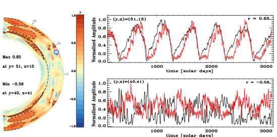
We now focus our attention on the relationship between⟨uθ⟩ and the toroidal field ⟨Bϕ⟩ that defines the large scale magnetic cycle. One of the first things that jumps to view is the morphology variations that happen to the MC during the cycle, inside an area defined by a cylinder parallel to the rotation axis and tangent to the tachocline at the equator (area between the rotation axis and the dotted vertical line in figure 1). At cycle maximum (figure 1C) there is the formation of a counter-clockwise rotating cell between 55◦ and 75◦ and another smaller clockwise rotating one at higher latitudes. Besides these morphological changes, the amplitude of⟨uθ⟩ in the region of the return flow at the base of the CZ, also varies in phase with ⟨Bϕ⟩ (see figure 2 right panels) as first noticed by Passos et al. (2012). The toroidal field seems to have an important role in modulating the horizontal component of the MC not only in the region of the return flow, but almost all over the convection zone. In order to get an idea of this close relationship, we present in figure 2 a correlation map between the amplitudes of⟨Bϕ⟩ and⟨uθ⟩. At mid to polar latitudes the correlation is mainly positive which means that the two amplitudes vary in phase. Outside the tangent cylinder, around 24◦ near the top layers there is a small patch where the correlation is negative. The time evolution of⟨Bϕ⟩ and ⟨uθ⟩ over sample period of ∼ 3000 solar days is shown in the right panels of figure 2. The areas with higher correlations (negative and positive) are marked with small colored circles (blue and yellow respectively).
Note that in the bottom return flow region, the toroidal field lags the meridional flow by more than∼ 6 solar days (months) which suggests a causal relationship.
Fol-60
30
0
Figure 2. Pearson correlation map, r, between the amplitudes of ⟨Bϕ⟩ and ⟨uθ⟩. The grid points of highest correlation and anti-correlations are marked by yellow and blue circles respectively. The panels on the right show the time evolution of the ⟨Bϕ⟩ (black) and ⟨uθ⟩ red for these two regions.
lowing these leads we look for a physical mechanism that could explain how the mag-netic field is influencing the MC. Notice that this simulation only goes up to 0.96 R⊙, which means that we don’t account for the surface layers nor we have active regions decays taking place.
3. Causes of MC variations
Since our simulation constitutes a closed system, the conservation of angular momen-tum, L, must be respected. Following Miesch & Hindman (2011) we look for the possibility that angular momentum variations due to local zonal forcing (axial torques) induces variations in the meridional flow (gyroscopic pumping). The equation that de-scribes the conservation of L in an anelastic system, is obtained by multiplying the zonal component of the momentum equation by r cosθ, and then average over longi-tude. For an inviscid simulation like ours (neglecting numerical diffusion), this yields
⟨ρ⟩∂L∂t + ⟨ρum⟩ · ∇L = −∇ ·
(
FRS+ FMS+ FMT)≡ F , (1) where⟨ρ⟩ is the reference ambient density and ⟨ρum⟩ · ∇L = FMCrepresents the
ad-vection ofL by meridional circulation, um, as a response to the net axial torqueF on
the r.h.s.. This net torque includes contributions from the Reynolds stresses, Maxwell stresses and mean magnetic fields (also called magnetic torque) that are individually defined as
FRS ≡ λ(⟨ρu′ru′ϕ⟩ ˆer+ ⟨ρu′θu′ϕ⟩ ˆeθ ) , FMS ≡ − λ µ0 ( ⟨b′rb′ϕ⟩ ˆer+ ⟨b′θb′ϕ⟩ ˆeθ ) , FMT ≡ −λ µ0 ( ⟨bϕbr⟩ˆer+ ⟨bϕbθ⟩ˆeθ⟩ ) .
This same approach was used by Miesch & Hindman (2011) to study how the MC is established in the solar near surface shear layer and by Featherstone & Miesch (2015) to study how it is established in hydrodynamic (non-magnetic) simulations of global convection. In the latter case, the Reynolds stress term has a preponderant role in establishing the overall morphology of the MC. In our case, we follow similar approach but using a fully MHD simulation with a large scale magnetic cycle built in. This allows us to assess the relationship between the magnetic field and the MC. the point of
A) B)
C)
30 30
60 60
0
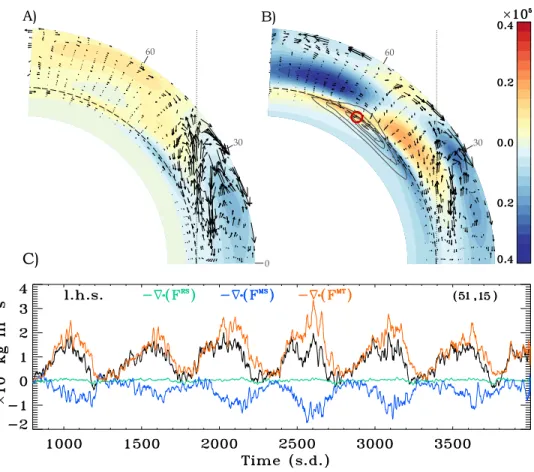
Figure 3. The divergence of the magnetic torque,−∇·FMTmapped in the northern hemisphere, at cycle minimum A) and maximum B). The vector field shows the direction of the meridional flow and the black contour lines in B) represent the area where the toroidal field accumulates. The red circle around 58◦near tachocline depth in B) represents
maximum correlation in this hemisphere. Panel C) shows the evolution of the l.h.s. of equation (1) and the individual contribution of 3 terms on the r.h.s. sampled at the red dot area over 7 cycles.
Figure 3C, shows the behaviour of the individual components of the net axial torque sampled at the ⟨uθ⟩ return flow at the bottom of the CZ. We can see that in this region, the magnetic torque has a maximal influence being somewhat opposed by the torque due to Maxwell stresses. These two terms clearly show the cycle modula-tion. This is because this area is where the magnetic field is accumulating. On the other hand, since this area is in the border between the stable and unstable layers, turbulence
is already weak and therefore the influence of the Reynolds stress is small. This demon-strates that in areas of high magnetic field accumulation, the large magnetic torque has a direct influence on the meridional circulation causally opposite to the behaviour com-monly characterizing the kinematic regime assumption.
Gyroscopic pumping induced MC variations depends on the strength of local torques, but these local forcings have a global effect due to mass conservation. We are currently investigating how the different terms contribute to the establishment of the global MC profile and how these variation affect the magnetic activity, closing in the loop (Passos et al. 2016) in prep.. The physical mechanism presented here might provide a consistent way of explaining the cyclic variations we observe in the MC.
Acknowledgments. D. Passos is thankful to Sandra Braz for support, and ac-knowledges the financial support from the Fundação para a Ciência e Tecnologia grant SFRH/BPD/68409/2010 (POPH/FSE), CENTRA-IST, the GRPS-UdeM and the Uni-versity of the Algarve for providing office space. P. Charbonneau is supported primarily by a Discovery Grant from the Natural Sciences and Engineering Research Council of Canada. All EULAG-MHD simulations reported upon in this paper were performed on the computing infrastructures of Calcul Québec, a member of the Compute Canada con-sortium. The National Center for Atmospheric Research is sponsored by the National Science Foundation.
References
Cameron, R. H., & Schüssler, M. 2010, ApJ, 720, 1030. 1007.2548 Featherstone, N. A., & Miesch, M. S. 2015, ApJ, 804, 67. 1501.06501 Ghizaru, M., Charbonneau, P., & Smolarkiewicz, P. K. 2010, ApJ, 715, L133 Hazra, G., Karak, B. B., & Choudhuri, A. R. 2014, ApJ, 782, 93. 1309.2838 Jackiewicz, J., Serebryanskiy, A., & Kholikov, S. 2015, ApJ, 805, 133 (9pp) Miesch, M. S., & Hindman, B. W. 2011, ApJ, 743, 79. 1106.4107
Passos, D., & Charbonneau, P. 2014, A&A, 568, A113
Passos, D., Charbonneau, P., & Beaudoin, P. 2012, Solar Phys., 279, 1
Passos, D., Charbonneau, P., & Miesch, M. 2015, ApJ, 800, L18. 1502.01154 Passos, D., Miesch, M., Charbonneau, P., & Guerrero, G. 2016, in prep.
Racine, É., Charbonneau, P., Ghizaru, M., Bouchat, A., & Smolarkiewicz, P. K. 2011, ApJ, 735, 46
Rajaguru, S. P., & Antia, H. M. 2015, ApJ, 813, 114 (8pp)
Smolarkiewicz, P. K., & Charbonneau, P. 2013, Journal of Computational Physics, 236, 608 Zhao, J., Bogart, R. S., Kosovichev, A. G., Duvall, T. L., Jr., & Hartlep, T. 2013, ApJ, 774, L29.