Central limit theorems for risk averse optimization problems

Funda¸c˜

ao Get´

ulio Vargas

Escola de Matem´

atica Aplicada

Matheus Secco Torres da Silva

Central limit theorems for risk averse optimization problems

Rio de Janeiro 2017

Matheus Secco Torres da Silva

Central limit theorems for risk averse optimization problems

Disserta¸c˜ao submetida `a Escola de

Matem´atica Aplicada como requisito parcial

para a obten¸c˜ao do grau de Mestre em

Modelagem Matem´atica da Informa¸c˜ao.

Orientador: Vincent G´erard Yannick Guigues

Rio de Janeiro 2017

Ficha catalográfica elaborada pela Biblioteca Mario Henrique Simonsen/FGV

Silva, Matheus Secco Torres da

Central limit theorems for risk averse optimization problems / Matheus Secco Torres da Silva. - 2017.

44 f.

Dissertação (mestrado) – Fundação Getulio Vargas, Escola de Matemática Aplicada.

Orientador: Vincent Gérard Yannick Guigues. Inclui bibliografia.

1. Programação estocástica. 2. Otimização matemática. 3. Administração de risco – Modelos matemáticos. I. Guigues, Vincent Gérard Yannick. II. Fundação Getulio Vargas. Escola de Matemática Aplicada. III. Título.

Agradecimentos

Gostaria de agradecer inicialmente a toda minha fam´ılia, em especial meus pais, Helcio e

Carla, meus av´os, Antˆonio, Lourdes, Helcio e M´arcia, a meus irm˜aos, Ian, Iasmin, Mayara e a

meu tio, Ricardo, que me introduziu neste bel´ıssimo mundo da Matem´atica.

Gostaria de agradecer tamb´em a minha noiva, Camilla, por todo apoio e compreens˜ao neste

per´ıodo em que estive escrevendo este trabalho.

Gostaria de agradecer profundamente a meu orientador, Vincent, por sua ajuda inestim´avel,

com todas as conversas, sugest˜oes e paciˆencia comigo.

Gostaria de agradecer a meus professores de Olimp´ıada no Ensino M´edio, por terem me

permitido al¸car vˆoos que eu nunca imaginara antes. Muito obrigado, Fabinho, Haroldo, Luciano,

Samuel e Yuri.

Por fim, gostaria de agradecer a todos os professores da EMAp por todos os cursos

ministra-dos, bem como aos meus professores da gradua¸c˜ao na PUC-Rio, que contribu´ıram imensamente

para a minha forma¸c˜ao matem´atica.

Sem todas essas pessoas, eu nunca chegaria aonde cheguei e por isso deixo aqui o meu imenso agradecimento.

Resumo

N´os estudaremos propriedades estat´ısticas de aproxima¸c˜oes pela m´edia amostral (SAA) de

problemas de otimiza¸c˜ao estoc´astica aversos ao risco. Inicialmente, discutimos alguns resultados

te´oricos importantes que ser˜ao ´uteis para a sequˆencia, como o Teorema Delta, o Teorema Central

do Limite Funcional e alguns resultados para o caso risco-neutro. Tamb´em lembramos a defini¸c˜ao

geral de medidas de risco, concentrando-nos nas medidas de risco poliedrais estendidas e nas medidas de risco coerentes ”law invariant”. Em seguida, obtemos teoremas centrais do limite

para os estimadores SAA dos valores ´otimos destes problemas, sob certas condi¸c˜oes impostas a

estas medidas de risco. Por fim, apresentamos resultados num´ericos para ilustrar os resultados te´oricos.

Abstract

We study statistical properties of the sample average approximation (SAA) of risk averse stochastic problems. We first introduce some background material, recalling important results for the continuation, such as the Delta Theorem, the Functional Central Limit Theorem, and asymptotics of risk-neutral problems. We also recall the concept of risk measures, focusing on two classes of risk measures: extended polyhedral risk measures (EPRMs) and law invariant coherent risk measures. We then provide central limit theorems for SAA estimators of the optimal values of stochastic programs expressed in terms of EPRMs or law invariant coherent risk measures, under certain assumptions on these risk measures. Numerical simulations illustrate the theoretical results.

Contents

1 Introduction 6

2 Statistical properties of SAA estimators of risk-neutral programs 8

2.1 Consistency of SAA estimators, unconstrained case . . . 9

2.2 Asymptotics of the SAA optimal value, unconstrained case . . . 12

2.3 Minimax stochastic programs . . . 15

2.4 Asymptotics of SAA optimal value, constrained case . . . 18

3 Risk measures 20 3.1 Coherent risk measures . . . 20

3.2 Examples of risk measures . . . 20

3.3 Dual representation of coherent risk measures . . . 23

3.4 Law invariant risk measures . . . 23

3.5 Extended polyhedral risk measures (EPRM) . . . 24

4 CLT for risk averse stochastic programs based on EPRM 24 4.1 Without constraints . . . 24

4.2 With constraints . . . 27

5 CLT for risk averse stochastic programs based on law invariant coherent risk measures 29 5.1 Without risk constraints . . . 29

5.2 With risk constraints . . . 31

6 Numerical simulations 33 6.1 Class of problems . . . 33

6.1.1 Constraint on AV@R of the portfolio return . . . 33

6.1.2 Constraint on the semi-deviation of the portfolio return . . . 34

6.2 Checking normality . . . 35

6.3 Confidence intervals . . . 39

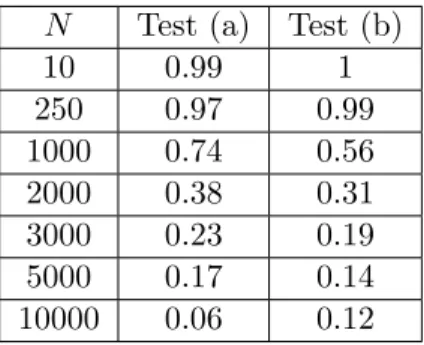
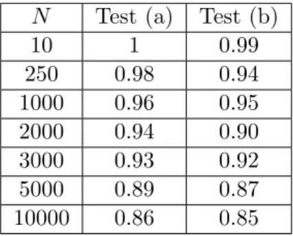
6.4 Hypothesis testing . . . 40

1

Introduction

An optimization problem consists in minimize or maximize a real function, defined in some domain. Our main interest is in stochastic optimization, which deals with problems that are not deterministic, i.e, that contains some randomness in its parameters. A simple example of stochastic optimization problem is the following portfolio problem: suppose that we want to

invest a capital C0 in n stocks (xi in each stock) and that the stock i has a return rate Ri. The

wealth after the investment is given by

C1=

n X i=1

⇠ixi,

where ⇠i = 1 + Ri (note that the return rates are random variables). One way to deal with this

problem is maximizing the expected value: 8 > > < > > : max x 0 E[C1], n X i=1 xi = C0.

Instead, a more conservative investor could want impose some control of the investment risk, using e.g the variance:

8 > > > > < > > > > : max x 0 E[C1], n X i=1 xi = C0, Var[C1] ⌫,

where ⌫ > 0 is a specified constant. In this work, we will deal with the following more general stochastic optimization problem:

#⇤ =

(

min_{R(g(x, ⇠)),}

x_{2 X,} (1)

where X is compact convex set in Rn, ⇠ is a random vector whose probability distribution is

supported on a set ⌅_{⇢ R}d_{, g(x, ⇠) :R}n_{⇥ ⌅ ! R is a Borel function which is convex in x for}

every ⇠ andR is a risk measure, which is used in general to determine some amount of the assets

to be kept in reserve. Also consider the constrained stochastic optimization problem:

#⇤= 8 > < > : minR[g(x, ⇠)], R[gi(x, ⇠)] 0, i = 1, ..., m, x2 X, (2)

where X, ⇠, g, _{R are as before, and g}i(x, ⇠) :Rn⇥ ⌅ ! R are also Borel functions which are

convex in x for every ⇠. Such problems can be hard to solve, because the objective function is in general complicated to describe. In order to deal with these difficulties, in [1], the sample

average approximation (SAA) to these problems was defined (we recall this definition in the following sections) and it allows us to tackle such problems through the use of sampling.

Our goal in this dissertation is to derive central limit theorems for SAA estimators of

prob-lems (1) and (2) when _{R is an extended polyhedral risk measure (EPRM) or a law invariant}

coherent risk measure. In the case of risk-neutral problems (when _{R = E), asymptotic and}

consistency properties of SAA estimator have been extensively studied. The asymptotic distri-bution of the empirical estimator in this case was proved in [3], [4], [5], [8], [13], [17], [20], and [21].

Some papers have treated the determination of nonasymptotic confidence intervals, i.e, when the sample size is fixed, on the optimal value of a stochastic program. In [18],the risk neutral case was studied using Talagrand inequality ([22]). Recently, in [10] the same problem was studied for EPRM using the Robust Stochastic Approximation and an extension of the Stochastic Mirror Descent Algorithm called Multistep Stochastic Mirror Descent as an alternative for estimating the optimal value of the problem.

In this context, the outline of our study is as follows. In Section 2, we introduce some fundamental tools such as Delta Theorem, Functional Central Limit Theorem and Danskin Theorem. Using these theorems, we establish results related to consistency of SAA estimators and central limit theorems for SAA estimators of constrained and unconstrained risk-neutral problems. In Section 3, we define coherent risk measures, introduced in [15], give examples of popular risk measures and verify which of these risk measures are coherent or not. We also give a dual representation of coherent risk measures, as well as the Kusuoka representation ([14]) for law invariant coherent risk measures and we recall the class of extended polyhedral risk measures (EPRM), introduced in [11]. In Section 4, we establish central limit theorems for problems of

type (1) and (2) when R is an EPRM. In Section 5, we establish new central limit theorems

for problems of type (1) and (2) when _{R is a law invariant coherent risk measure, using results}

established in [9]. In Section 6, we consider two portfolio problems and we perform numerical simulations on these problems in order to illustrate our theoretical results. More precisely, we provide QQ-plots and apply Jarque-Bera test to verify asymptotic normality of the distribution of the empirical optimal value. We also report asymptotic confidence intervals and perform hypothesis testing in order to compare the optimal values of both problems.

We will use the following notation and terminology: • R - set of real numbers.

• N = {0, 1, 2, . . .} - set of natural numbers. • E[X] - expected value of random variable X. • Var[X] - variance of random variable X.

• C(X) - space of continuous real-valued functions in X.

• N (µ, 2_{) - normal distribution with mean µ and variance} 2_.

• For a nonempty set X ⇢ Rn_{, the polar cone X}⇤ _{is defined by X}⇤ _={x⇤ _{:hx, x}⇤_{i  08x 2}

• u+= max(u, 0).

• Let (Xk) and (Zk) be sequences of random variables. We write Zk = Op(Xk) if for any

" > 0, there exists c > 0 such that P (_|Zk/Xk| > c)  " for all k 2 N. Also Zk = op(Xk) means that for any " > 0 we have limk!1P (|Zk/Xk| > ") = 0.

2

Statistical properties of SAA estimators of risk-neutral

pro-grams

This section follows Chapter 5 of [1]. The proofs of this section are also taken from this reference. In this section, we recall some results for risk-neutral programs, which will be used to derive the results of Section 4. Consider the following stochastic optimization problem:

min

x2X{f(x) := E [F (x, ⇠)]} . (3)

Here, X is a nonempty closed subset ofRn, ⇠ is a random vector whose probability distribution

is supported on a set ⌅_{⇢ R}dand F : X_{⇥ ⌅ ! R is a Caratheod´ory function, i.e, continuous in}

x and measurable in ⇠. We also assume that the expectation function f (x) is well defined and

finite value for all x 2 X. In order to get estimates of the optimal value of this problem, we

solve the SAA which uses a sample ⇠1, . . . , ⇠N of N realizations of random vector ⇠:

Definition 2.1. The SAA of problem (3) is the optimization problem min x2X 8 < :fˆN(x) := 1 N N X j=1 F (x, ⇠j) . 9 = ; (4)

The random vectors (⇠1, . . . , ⇠N) in (4) are i.i.d (independent and identically distributed) and

have the distribution of ⇠ in (3).

Note that we can view the sample average functions ˆfN(x) as defined on a common

prob-ability space (⌦,F, P ), where F is a sigma algebra on ⌦ and P is a probability measure. For

example, in the case of a i.i.d sample, one possible construction is to take the set ⌦ := ⌅1 of

sequences_{⇠1, . . .}⇠i2⌅,i2N. We recall the Strong Law of Large Numbers that will be used in the

continuation:

Theorem 2.1. (Strong Law of Large Numbers) Let X1, X2, . . . be a sequence of independent

random variables on some probability space. If X1, X2, . . . are i.i.d and have finite first moment

E[X1] = µ, then P ✓ lim n!+1 X1+ . . . + Xn n = µ ◆ = 1. Proof. See [16]. ⇤

By the Strong Law of Large Numbers, when the sample is i.i.d, we have that ˆfN(x) converges

pointwise with probability (w.p.) 1 to f (x), as N goes to +_{1. In what follows, we will also use}

Definition 2.2. (Uniform convergence w.p. 1) We say that ˆfN(x) converges uniformly to f (x)

w.p. 1 on X if for almost every !_{2 ⌦, we have that:}

lim

N!+1_x2Xsup

ˆ

fN(x, !) f (x) = 0 (5)

Definition 2.3. We say that F (x, ⇠), x_{2 X, is dominated by an integrable function when there}

is a nonnegative valued measurable function g(⇠) such that _{E [g(⇠)] < +1 and for all x 2 X,}

the inequality |F (x, ⇠)|  g(⇠) holds w.p. 1.

With these definitions, we can state the Uniform Law of Large Numbers (Jennrich [12]), which is a useful criterion to ensure uniform convergence w.p. 1 for the sequence of functions

ˆ fN(x):

Theorem 2.2. (Uniform Law of Large Numbers) Let X be a nonempty compact subset of Rn

and suppose that:

(i) For any x_{2 X, the function F (., ⇠) is continuous at x for almost every ⇠ 2 ⌅.}

(ii) F (x, ⇠), x2 X, is dominated by an integrable function.

(iii) The sample is i.i.d.

Then the expected value function f (x) = _{E[F (x, ⇠)] is finite valued and continuous on X, and}

ˆ

fN(x) converges uniformly to f (x) w.p. 1.

2.1 Consistency of SAA estimators, unconstrained case

In this section we discuss convergence properties of the SAA estimators of the optimal value and of the optimal solutions. For the continuation, we introduce some definitions:

Definition 2.4. We denote by #⇤ _{and S the optimal value and the set of optimal solutions,}

respectively, of true problem (3). Also, we denote by ˆ#N and ˆSN the optimal value and the set

of optimal solutions, respectively, of SAA problem (4).

Definition 2.5. We say that estimator ˆ✓N of ✓ is consistent if ˆ✓N converges w.p. 1 to ✓ as

N _{! +1.}

We can now state a theorem ensuring the consistency of estimator ˆ#N of #⇤:

Theorem 2.3. Suppose that ˆfN(x) converges to f (x) w.p. 1 as N ! +1, uniformly on X.

Then ˆ#N converges to #⇤ w.p. 1, i.e, ˆ#N is a consistent estimator of #⇤.

Proof. By the uniform convergence w.p. 1, we have that for any " > 0 and a.e. ! 2 ⌦,

9N⇤ = N⇤(", !) such that for all N N⇤:

sup x2X

ˆ

Let x⇤ be such that f (x⇤) = #⇤ and ˆxN such that ˆfN(ˆxN, !) = ˆ#N(!). Hence, we have that: ˆ

#N(!) ˆfN(x⇤, !) f(x⇤) + ". (7)

ˆ

#N(!) = ˆfN(ˆxN, !) f (ˆxN) " f (x⇤) ". (8)

By (7) and (8), we have that ˆ#N(!) #⇤  " and ˆ#N(!) #⇤ " and hence

ˆ

#N(!) #⇤  " (9)

As " is arbitrary, this completes the proof. ⇤

We are now about to discuss the consistency of the SAA estimators of the optimal solutions, which will be expressed using the concept of deviation between two sets:

Definition 2.6. Given two sets A and B, the deviation of set A from set B is denoted by D(A, B) := sup

x2A

dist(x, B). (10)

By the definition, dist(x, A) = +1 if A is empty and hence D(A, B) = +1 if B is empty.

Remark 2.1. By definition, dist(x, A) = +_{1 if A is empty and hence D(A, B) = +1 if B is}

empty.

We will make use of the following proposition:

Proposition 2.1. Let f : X _{! R and f}N : X ! R be a sequence of deterministic real valued

functions. Then the following two properties are equivalent:

(i) For any x _{2 X and any sequence {x}N} ⇢ X converging to x, it follows that fN(xN)

converges to f (x).

(ii) The function f is continuous on X and fN converges to f uniformly on compact subsets

of X.

Proof. Suppose that property (i) holds. We will first prove that f is continuous. For this,

take x 2 X, a sequence (xN) ⇢ X converging to x, and " > 0 arbitrary. By taking the

constant sequence with all terms equal to x1, we have by (i) that fN(x1)! f(x1). Hence, there

exists N1 such that |fN1(x1) f (x1)| < "

2. In the same way, there exists N2 > N1 such that

|fN2(x2) f (x2)| < "₂ and so on. Consider now the sequence x0N constructed in the following

way: x0_i = x1, i = 1, . . . , N1, x0i = x2, i = N1 + 1, . . . , N2, and so on. Clearly, this sequence is

such that x0_{n ! x and therefore we have by property (i) that |f}N(x0N) f (x)| < 2" for all N

sufficiently large. By construction of Nk, we have that |fNk(xk) f (xk)| <

"

2. Note also that

fNk(xk) = fNk(x0Nk), because xk= x 0

Nk and hence fNk(x0Nk) f (xk) < "

2. With this, we have

that for every sufficiently large k:

|f(xk) f (x)|  f(xk) fNk(x0Nk) + fNk(x0Nk) f (x) < "

2 +

"

Since " is arbitrary, this proves that f (xk)! f(x) and therefore f is continuous on x. Since x is arbitrary, we have that f is continuous on X.

Now let K be a compact subset of X. Suppose for the sake of the contradiction that fN

does not converge to f uniformly on K. Therefore, there exists " > 0 and a sequence (xN)⇢ K

such that _|fN(xN) f (xN)| " for every N . By passing to a subsequence, if necessary, Since

K is compact, we can assume that xN ! x 2 K. By the triangular inequality, it follows that:

|fN(xN) f (xN)|  |fN(xN) f (x)| + |f(x) f (xN)| . (12)

The first term on the right-hand side of this inequality converges to 0 due to property (i) and the second term also converges to 0 because of the continuity of f and hence for sufficiently

large N , we have that_|fN(xN) f (xN)| < ", which yields a contradiction.

Now assume that property (ii) holds. Let (xN) ⇢ X be a sequence converging to x 2 X.

Clearly, we can suppose that this sequence is contained in a compact subset of X. Using again the triangular inequality, we have that:

|fN(xN) f (x)|  |fN(xN) f (xN)| + |f(xN) f (x)| . (13)

The first term in the right-hand side of this inequality converges to 0 because of the uniform

convergence of fN to f on compact subsets of X and the second term converges to 0 because of

the continuity of f , and both are guaranteed due to property (ii). ⇤

Now we can establish the following result on the consistency of SAA estimators:

Theorem 2.4. Suppose that there exists a compact set C_{⇢ R}n _{such that:}

(i) The set S of optimal solutions of the true problem (3) is nonempty and contained in C. (ii) The function f (x) is finite valued and continuous on C.

(iii) ˆfN(x) converges to f (x) w.p. 1, as N ! 1, uniformly in x 2 C.

(iv) With probability 1, for N large enough, the set ˆSN of optimal solutions of the SAA is

nonempty and ˆSN ⇢ C.

Then ˆ#N ! #⇤ andD( ˆSN, S)! 0 w.p. 1 as N ! 1.

Proof. By assumptions (i) and (iv), we can assume that SAA problem is restricted to the set

X\ C. Therefore, without loss of generality, we can suppose that X is compact. The assertion

ˆ

#N ! #⇤ is ensured by Theorem 2.3 due to assumption (iii). Now it is sufficient to prove

that D( ˆSN(!), S) ! 0 for every ! 2 ⌦ such that ˆ#N(!) ! #⇤ and assumptions (iii) and (iv)

hold. This is basically a deterministic result; therefore, we omit ! for the sake of notational

convenience. Let us argue by contradiction. Suppose thatD( ˆSN, S) does not converges to 0 as

N goes to_{1. Because X is compact, by passing to a subsequence, if necessary, we can assume}

that there exists ˆxN 2 ˆSN such that dist(ˆxN, S) " for some " > 0 and that ˆxN converges to a

point x⇤ 2 X. It follows that x⇤_{62 S and hence f(x}⇤_{) > #}⇤_{. Moreover, ˆ#}

N = ˆfN(ˆxN) and using

assumptions (ii) and (iii) and Proposition 2.1, we have that ˆfN(ˆxN)! f(x⇤). Hence we obtain

that ˆ#N converges to f (x⇤) > #⇤, a contradiction.

Consistency of SAA estimators shows that, for large sample sizes N , ˆ#N provides a good

approximation of the optimal value #⇤ _{of (3). In the next section, we study the asymptotic}

distribution of the estimator ˆ#N of #⇤.

2.2 Asymptotics of the SAA optimal value, unconstrained case

We start showing that estimator ˆ#N of #⇤ is biased:

Proposition 2.2. Let ˆ#N be the optimal value of SAA problem (4) and suppose that the sample

is i.i.d.. Then E[ˆ#N] E[ ˆ#N +1] #⇤ for any N 2 N.

Proof. We first prove that _E[ˆ#N] #⇤ for any N 2 N. For this, since ˆ#N = inf

x2X ˆ

fN(x), we have

that ˆfN(x) #ˆN for every x2 X. Taking the expected value on both sides and minimizing the

left side over x, we have

inf

x2XE[ ˆfN(x)] E[ˆ#N]. (14)

Because the sample is i.i.d., it follows that E[ ˆfN(x)] = f (x) and since inf

x2Xf (x) = #

⇤_{, we have}

thatE[ˆ#N] #⇤.

Now it remains to prove thatE[ˆ#N] E[ ˆ#N +1]. First observe that

ˆ fN +1(x) = 1 N + 1 N +1_X i=1 2 4 1 N X j6=i F (x, ⇠j) 3 5 . Moreover, since the sample is i.i.d. we have

E[ˆ#N +1] =E h

inf_x2XfˆN +1(x) i

= Ehinf_{x2X N +1}1 PN +1_i=1 ⇣_N1 P_j6=iF (x, ⇠j)⌘i

Eh 1 N +1 PN +1 i=1 ⇣ infx2X N1 P j6=iF (x, ⇠j) ⌘i = _{N +1}1 PN +1_i=1 Ehinf_{x2X N}1 P_j6=iF (x, ⇠j)i = _{N +1}1 PN +1_i=1 E[ˆ#N] =E[ˆ#N],

which ends the proof. ⇤

Theorem 2.5. (Central limit theorem - CLT) Let X1, X2, . . . be a sequence of independent

random variables on some probability space. If X1, X2, . . . are i.i.d and have finite meanE[X1] =

µ and finite variance Var[X1] = 2, defining Mn:= X1+...+X_n n, we have that

p

n(Mn µ) D

! N (0, 1),

where D_{! denotes convergence in distribution.}

Let us now turn to the study of first order asymptotics of the SAA optimal value. Note first

that for fixed x_{2 X, the sample average estimator ˆ}fN(x) of f (x) is unbiased and has variance

2_{(x)/N where} 2_{(x) := Var[F (x, ⇠)] is supposed to be finite. Moreover, by the CLT we have}

that

N1/2hfˆN(x) f (x)

i _D

! Yx, (15)

where Yx has normal distribution with mean 0 and variance 2(x), written Yx ⇠ N (0, 2(x)).

We will also use the notation Yx = Y (x).

To proceed, we need a functional central limit theorem (see Araujo and Gin´e [2], Corollary 7.17).

Definition 2.7. A sequence of random elements{Xn: n 1} of a metric space (S, m) converges

in distribution to a random element X of (S, m) if and only if lim

n!+1E[f(Xn)] =E[f(X)] for all f 2 C(S), (16)

where C(S) is the space of continuous, bounded, real-valued functions on S.

Theorem 2.6 (Functional CLT). Consider F : X⇥⌅ ! R a Caratheod´ory function satisfying

the following assumptions:

A-1 for some point x2 X, the expectation E[F (x, ⇠)2_{] is finite.}

A-2 There exists a measurable function L : ⌅_{! R}+ such that E[L(⇠)2] is finite and

F (x, ⇠) F (x0, ⇠) _{ L(⇠)kx} x0_k (17)

for all x, x0 2 X and a.e ⇠ 2 ⌅.

Suppose that X is compact and the sample ⇠1, . . . , ⇠N of N realizations of random vector ⇠ is

i.i.d. We recall that f (x) =E[F (x, ⇠)] and that ˆfN(x) is the SAA of f (x). Then N1/2( ˆfN f )

converges in distribution to Y , viewed as a random element of C(X), i.e, Y is a mapping

Y : ⌦! C(X) from a probability space (⌦, F, P ) into C(X) which is measurable with respect to

the Borel sigma algebra of C(X), i.e, Y (x) = Yx= Y (x, !) can be viewed as a random function.

Moreover, we have that Y is a Gaussian process:

(i) For any x1, . . . , xn2 X and any real numbers t1, . . . , tn, n X

i=1

tiY (xi) is Gaussian.

(ii) For any x_{2 X, E[Y (x)] = 0.}

(iii) For any x, x0 2 X, E[Y (x)Y (x0_{)] = Cov(F (x, ⇠), F (x}0_{, ⇠)).}

Definition 2.8. Let B1 and B2 be two Banach Spaces, and let G : B1 ! B2 be a mapping. We

say that G is directionally di↵erentiable at µ_{2 B}1 if the limit

G0_µ(d) := lim t#0

G(µ + td) G(µ)

exists for all d_{2 B}1. Moreover, we say that G is directionally di↵erentiable at µ in the sense of

Hadamard if the directional derivative G0

µ exists for all d2 B1 and

G0_µ(d) = lim t#0 d0_!d

G(µ + td0) G(µ)

t .

Definition 2.9. Given a function f : X ! Y , the arg min over some subset S of X is defined

as

argmin x2S

f :=_{{x 2 S|8y 2 S : f(y)  f(x)}.}

We need the following theorem by Danskin, see [6].

Theorem 2.7 (Danskin). Let X be a metric space and U be a normed space. Suppose that

for all x_{2 X the function f(x, .) is di↵erentiable, in the sense of Fr´echet, and that f(x, u) and}

Duf (x, u) are continuous on X ⇥ U, and let be a compact subset of X. Then the optimal

value function v(u) := inf_x2 f (x, u) is Hadamard directionally di↵erentiable and

v_u0(d) = inf

x2S(u)Duf (x, u)d,

where S(u) is the set argmin_u2Uf (x, u).

Theorem 2.8 (Delta Theorem). Let B1 and B2 be Banach Spaces, equipped with their Borel

-algebras, YN be a sequence of random elements of B1, G : B1 ! B2 be a mapping, and

⌧N be a sequence of positive numbers tending to infinity as N ! 1. Suppose that the space

B1 is separable, i.e, it has a countable dense subset, the mapping G is Hadamard directionally

di↵erentiable at a point µ2 B1, and the sequence XN := ⌧N(YN µ) converges in distribution

to a random element Y of B1. Then

⌧N[G(YN) G(µ)] D! G0µ(Y )

and

⌧N[G(YN) G(µ)] = G0µ(XN) + op(1).

We are now in a position to prove a Central Limit Theorem for SAA estimator ˆ#N of #⇤:

Theorem 2.9. Let ˆ#N be the optimal value of SAA problem (4). Suppose that the sample is

i.i.d., the set X is compact, and Assumptions A-1 and A-2 (in Theorem 2.6) are satisfied. Then the following holds:

ˆ #N = inf x2S ˆ fN(x) + op(N 1/2) and (18) N1/2( ˆ#n #⇤) D! inf x2SY (x). (19)

If moreover, S =_{{x} is a singleton, then}

Proof. The key ingredients to the proof are Danskin Theorem, Functional CLT, and Delta

Theorem. Consider Banach Space C(X) of continuous functions : X _{! R equipped with the}

sup-norm k k = supx2X| (x)|. Define the min-value function V ( ) := infx2X (x). Since X is

compact, the function V : C(X)_{! R is real valued and measurable (with respect to the Borel}

sigma algebra of C(X)). By Danskin theorem, V (_{·) is Hadamard directionally di↵erentiable and}

V_µ0( ) = inf

x2X(µ)

(x), _{8 2 C(X),} (21)

where X(µ) := argmin_x2Xµ(x). As the hypotheses of Funcional CLT are satisfied, then

N1/2( ˆfN f ) converges in distribution to the random element Y of C(X). Since X is compact,

C(X) is separable by Stone-Weierstrass theorem and hence we can apply the Delta theorem to

the min-function V (_{·) at µ = f. Noting that ˆ}#N = V ( ˆfN), #⇤ = V (f ) and X(f ) = S and using

(21), we obtain (19) and ˆ

#N #⇤ = inf

x2S[ ˆfN(x) f (x)] + op(N

1/2_{). (22)}

Since f (x) = #⇤ for any x_{2 S, (22) is equivalent to (18). Finally (20) follows immediately from}

(19). ⇤

2.3 Minimax stochastic programs

Let us consider the following minimax stochastic program, which will be useful later for con-strained problems:

min

x2Xsup_y2Y{f(x, y) := E[F (x, y, ⇠)]}, (23)

where X ⇢ Rn _{and Y ⇢ R}m _{are closed sets, F : X⇥ Y ⇥ ⌅ ! R, and ⇠ = ⇠(!) is a random}

vector whose probability distribution is supported on ⌅_{⇢ R}d. The corresponding SAA problem

is as follows: min x2Xsup_y2Y{ ˆfN(x, y) := 1 N N X j=1 F (x, y, ⇠j)}. (24)

As before, denote by #⇤and ˆ#N the optimal values of (23) and (24), respectively, and by Sx⇢ X

and ˆSx,N the respective set of optimal solutions.

Definition 2.10. A function F (x, y, ⇠) is said to be a Carath´eodory function if F (x, y, ⇠(·)) is

measurable for every (x, y,_{·) and F (·, ·, ⇠) is continuous for a.e ⇠ 2 ⌅.}

We make the following assumptions: (A’1) F (x, y, ⇠) is a Carath´eodory function. (A’2) X, Y are nonempty and compact.

(A’3) There exists an open set N _{⇢ R}m+n_{such that X⇥ Y ⇢ N and there exists an integrable}

Because of Theorem 7.48 in [1], it follows that f (x, y) is continuous on X_{⇥Y . Since Y is compact,}

this implies that the max-function (x) := sup_y2Y f (x, y) is continuous on X. Furthermore, it

also follows that the function ˆfN(x, y) = ˆfN(x, y, !) is a Carath´eodory function and hence the

sample average max-function ˆN(x, !) := supy2Y fˆN(x, y, !) is also a Carath´eodory function.

Since ˆ#N = ˆ#N(!) is given by the minimum of the Carath´eodory function ˆN(x, w), it follows

that it is measurable. Now we give, as in Theorems 2.3 and 2.4, a result on the consistency of the SAA estimators:

Theorem 2.10. Suppose that Assumptions (A’1)-(A’3) hold and that the sample is i.i.d. Then ˆ

#N ! #⇤ and D( ˆSx,N, Sx)! 0 w.p. 1 as N ! 1.

Proof. By the Uniform Law of Large Numbers, we have that under the specified assumptions ˆ

fN(x, y) converges to f (x, y) w.p. 1 uniformly on X⇥ Y . Defining

N := sup

(x,y)2X⇥Y

ˆ

fN(x, y) f (x, y) ,

we have that N ! 0 as N ! 1. Consider ˆN(x) := supy2Y fˆN(x, y) and (x) := supy2Y f (x, y).

We have that

sup x2X

ˆ_{N(x) (x)  N,}

and hence ˆ#N #⇤  N, which implies that ˆ#N ! #⇤ w.p. 1 as N ! 1. The function

(x) is continuous and ˆN(x) is continuous w.p. 1. Consequently, Set Sx is nonempty and ˆSx,n

is nonempty w.p. 1. Now the relation _{D( ˆ}Sx,N, Sx) ! 0 can be shown following the proof of

Theorem 2.4. ⇤

We discuss now asymptotic results on ˆ#N. We make the following additional assumptions:

(A’4) The sets X and Y are convex, and for a.e ⇠2 ⌅ the function F (·, ·, ⇠) is convex-concave

on X _{⇥ Y , i.e, the function F (·, y, ⇠) is convex on X for every y 2 Y and the function}

F (x,_{·, ⇠) is concave on Y for every x 2 X.}

It follows that the expected value f (x, y) is convex concave and continuous on X_{⇥ Y . We now}

use von Neumann’s Minimax Theorem.

Theorem 2.11 (von Neumann’s Minimax Theorem, [7]). Let V and W be two reflexive Banach

spaces and let M ⇢ V and N ⇢ W be two closed convex nonempty sets. Let L : M ⇥ N ! R be

a bivariate function which satisfies the following properties:

(i) _{8w 2 N, L(., w) is convex and lower semicontinuous on M.}

(ii) 8v 2 M, L(v, .) is concave and upper semicontinuous on N.

(iii) M and N are bounded.

Then L possesses a saddle point (v, w)_{2 M ⇥ N, i.e,}

min

Remark 2.2. In particular, infvsupwL(v, w) = supwinfvL(v, w), i.e, there is no duality gap. By von Neumann’s theorem, we have that problem (23) and its dual

max

y2Y x2Xinf f (x, y) (25)

have non empty and bounded sets of optimal solutions, Sx ⇢ X and Sy ⇢ Y , respectively.

Moreover, the optimal values of problems (23) and (25) are equal to each other and Sx ⇥ Sy

forms the set of saddle points of these problems.

(A’5) For some point (x, y)_{2 X ⇥ Y , the expectation E[F (x, y, ⇠)}2] is finite, and there exists a

measurable function C : ⌅_{! R}+ such that E[C(⇠)2] is finite and the inequality

F (x, y, ⇠) F (x0, y0, ⇠)  C(⇠) kx x0k + ky y0k

holds for all (x, y), (x0, y0)2 X ⇥ Y and a.e ⇠ 2 ⌅.

The above assumption implies that f (x, y) is Lipschitz continuous on X _{⇥ Y with Lipschitz}

constant  =_{E[C(⇠)]. We now prove a theorem similar to Theorem 2.9. In order to prove this}

theorem, we will need the following tangential version of Delta theorem, which can be found in [1].

Theorem 2.12 (Delta Theorem - tangential version). Let B1 and B2 be Banach spaces, K be

a subset of B1, G : B1 ! B2 be a mapping, and YN be a sequence of random elements of B1.

Suppose that the following assumptions hold:

(i) The space B1 is separable.

(ii) The mapping G is Hadamard directionally di↵erentiable at a point µ tangentially to the set K.

(iii) For some sequence ⌧N of positive numbers tending to infinity, the sequence XN := ⌧N(YN

µ) converges in distribution to a random element Y .

(iv) YN 2 K w.p. 1 for all N large enough.

Then

⌧N[G(YN) G(µ)] ! GD 0µ(Y ).

Moreover, if the set K is convex, then

⌧N[G(YN) G(µ)] = G0µ(XN) + op(1).

Remark 2.3. We say that G is Hadamard directionally di↵erentiable at a point µ tangentially

to a set K ⇢ B1 if for any sequence dN of the form dN := yN_tNµ, where yn 2 K, tN # 0, and

such that dN ! d, the following limit exists:

G0_µ(d) = lim

N!+1

G(µ + tNdN) g(µ)

tN

Theorem 2.13. Consider the minimax stochastic problem (23) and its SAA problem (24) based on an i.i.d. sample. Suppose that Assumptions (A’1)-(A’2) and (A’4)-(A’5) hold. Then

ˆ #N = inf x2Sx sup y2Sy ˆ fN(x, y) + op(N 1/2).

Moreover, if Sets Sx = {x} and Sy = {y} are singletons, then N1/2( ˆ#N #⇤) converges in

distribution to N (0, 2_{), where} 2 _{= Var[F (x, y, ⇠)].}

Proof. Consider the space C(X, Y ) of continuous functions : X⇥ Y ! R equipped with the

sup-norm_{k k = supx2X,y2Y | (x, y)|, which is separable by Stone-Weierstrass theorem, because}

X and Y are compact, and Set_{K of convex-concave functions on X ⇥Y is contained in C(X, Y ).}

It is not difficult to see thatK is a closed (in the norm topology of C(X, Y )) and convex cone.

Consider the optimal value function V : C(X, Y )_{! R defined as}

V ( ) := inf x2Xsupy2Y

(x, y) for 2 C(X, Y ).

By Theorem 7.24 in [1], we have that the optimal value function V (_{·) is Hadamard directionally}

di↵erentiable at f tangentially to the setK and

V_f0( ) = inf

x2Sx

sup y2Sy

(x, y). (26)

Because of assumption (A’5) we have, by Theorem 2.6, that N1/2_{( ˆf}

N f ), considered as a

sequence of random elements of C(X, Y ), converges in distribution to a random element of

C(X, Y ). Then by noting that #⇤ = f (x⇤, y⇤) for any (x⇤, y⇤) _{2 S}x⇥ Sy, and using Equation

(26) together with the tangential version of Delta theorem achieves the proof of the theorem. ⇤

2.4 Asymptotics of SAA optimal value, constrained case

The previous section allows us to derive asymptotics for constrained stochastic programs. More precisely, we consider the following problem:

8 > < > : min_{{f(x) = E[F (x, ⇠)]}} gi(x) =E[Gi(x, ⇠)] 0, i = 1, ..., p, x2 X, (27)

where X is a nonempty, closed, and convex subset of Rn, and F, Gi : X⇥ ⌅ ! R, i = 1, . . . , p.

We assume that for all ⇠ 2 ⌅, the functions F (·, ⇠) and Gi(·, ⇠), i = 1, ..., p are convex. The

Lagrangian function of this problem is

L(x, ) := f (x) + p X

i=1

igi(x).

We assume that functions f (x) and gi(x) are finite valued on a neighborhood of the set S of

associated a nonempty and bounded set ⇤ of Lagrange multipliers = ( 1, . . . , p) satisfying the optimality conditions

x_{2 argmin}

x2X

L(x, ), i 0, and igi(x) = 0, i = 1, ..., p

The set ⇤ coincides with the set of optimal solutions of the dual of the true problem and therefore

is the same for any optimal solution x_{2 S.}

Let now ˆ#N be the optimal value of the following SAA problem of problem (27):

8 > < > : min ˆfN(x) ˆ giN(x) 0, i = 1, ..., p, x_{2 X} (28)

where ˆfN(x) is defined as in (4) and

ˆ giN(x) = 1 N N X j=1 Gi(x, ⇠j).

Assume now that Conditions A-1 and A-2 stated in Theorem 2.6 hold for integrands F and

Gi, i = 1, ..., p. It follows that the corresponding expected value functions f (x) and gi(x) are

finite valued and continuous on X. As in Theorem 2.9, we denote by Y (x) random variables which are normally distributed and have the same covariance structure as F (x, ⇠). We also

denote by Yi(x) random variables which are normally distributed and have the same covariance

structure as Gi(x, ⇠), i = 1, ..., p.

Theorem 2.14. Let ˆ#N be the optimal value of SAA problem (28). Suppose that the sample is

i.i.d., the problem is convex, and the following conditions are satisfied: 1. the set S, of optimal solutions, is nonempty and bounded.

2. the functions f (x) and gi(x) are finite valued on a neighborhood of S.

3. the Slater condition for the true problem holds, that is, there exists a point x⇤ _{2 X such}

that gi(x⇤) < 0, i = 1, . . . , p.

4. Assumptions A-1 and A-2 hold for integrands F and Gi, i = 1, ..., p.

Then N1/2⇣#ˆN #⇤ ⌘ _D ! inf x2Ssup_2⇤ " Y (x) + p X i=1 iYi(x) # . (29)

If, moreover, S =_{{x} and ⇤ = { }, then}

N1/2⇣#ˆN #⇤ ⌘ _D ! N (0, 2), (30) with 2_{:= Var} " F (x, ⇠) + p X i=1 iGi(x, ⇠) # .

3

Risk measures

In this chapter, we introduce the concept of a risk measure, which will be used in Sections 4

and 5. Let (⌦,_{F) be a sample space, with F a sigma algebra, on which uncertain outcomes are}

defined (random functions Z = Z(!)).

Definition 3.1. A risk measure is a function ⇢(Z) which maps a random variable Z into the

extended real line_{R = R [ {+1} [ { 1}.}

The space_{Z of allowable functions will be Z = L}p(⌦,F, P), with 1  p  +1. This means

that Z(!) has a finite p-th order moment with respect to the reference probability measure P .

We assume that risk measures ⇢ : Z ! R are proper, i.e, ⇢(Z) > 1 for every Z 2 Z and

dom(⇢) :=_{{Z 2 Z : ⇢(Z) < +1} is nonempty.}

3.1 Coherent risk measures

It has been agreed by Artzner et al [15] that ”good” risk measures, in the sense that investors agree that risk measures should satisfy these properties, called coherent in [15], should have the following properties:

Definition 3.2. We say that ⇢ is a coherent risk measure if satisfies the following conditions: (R1) Convexity:

⇢(tZ + (1 t)Z0)_{ t⇢(Z) + (1} t)⇢(Z0)

for all Z, Z0 _{2 Z and all t 2 [0, 1].}

(R2) Monotonicity: If Z, Z0 _{2 Z and Z} Z0 (Z(!) Z0(!) for a.e !_{2 ⌦), then ⇢(Z)} ⇢(Z0).

(R3) Translation equivariance: if a_{2 R and Z 2 Z, then ⇢(Z + a) = ⇢(Z) + a.}

(R4) Positive Homogeneity: if t > 0 and Z 2 Z, then ⇢(tZ) = t⇢(Z).

3.2 Examples of risk measures

We now give examples of popular risk measures.

Example 3.1 (Upper semideviations of order p). The upper semideviation of order p is defined as

+

p[Z] = E

⇥

(Z E[Z])p₊⇤ 1/p,

where (a)+ = max{a, 0} and 1  p  +1 is a fixed parameter. We assume that the random

variables Z : ⌦_{! R are defined on L}p(⌦,F, P) and so Z has finite p-th order moment.

Proposition 3.1. The semideviation of order p satisfies Conditions (R1) and (R4), but does not satisfy Conditions (R2) and (R3).

Proof. It is immediate that (R4) holds. We will prove now that (R1) holds. By Minkowski inequality, we have that for random variables X and Y :

E⇥(X)p₊⇤ 1/p+ E⇥(Y )₊p⇤ 1/p (E [((X)++ (Y )+)p])1/p.

Now we use that (a)++ (b)+ (a + b)+ for all real numbers a and b. This is indeed equivalent

to the triangle inequality|a| + |b| |a + b|. Hence we have that:

(E [((X)++ (Y )+)p])1/p (E [((X + Y )+)p])1/p. Using the last two inequalities, we have that:

E⇥(X)p₊⇤ 1/p+ E⇥(Y )p₊⇤ 1/p (E [((X + Y )+)p])1/p.

Replacing X = t(Z E[Z]) and Y = (1 t)(Z0 E[Z0]), t 2 [0, 1], we get (R1). Condition

(R3) is clearly not satisfied, because +_p[Z + a] = +_p[Z] for all a 2 R. Finally, we show that

(R2) is not satisfied. Indeed, take discrete random variables Z and Z0 such that P (Z = 0) = 0

and P (Z = 1) = 1 and P (Z0 = 1) = P (Z0 = 0) = 1₂. Hence E[Z] = 1 and _p+[Z] = 0. On

the other hand, E[Z0] = 1₂ and therefore _p+[Z0] = 1₂ p+1p _{. For this example, Z Z}0 _but

+

p [Z] < p+[0Z0]. ⇤

Example 3.2 (Value-at-Risk - V@R). If Z is a random variable which represents losses, we

define the Value-at-Risk of Z at the confidence level 1 ↵ as

V@R↵(Z) = inf{` 2 R : P (Z > `)  ↵}.

Note that losses larger than V@R↵(Z) occur with probability less than or equal to ↵.

Proposition 3.2. The Value-at-Risk satisfies Conditions (R2), (R3), and (R4), but does not satisfy Condition (R1).

Proof. It is clear that V@R↵(Z) satisfies (R3) and (R4). Let us now prove that Condition

(R2) holds. For this, let Z and Z0 be such that Z Z0. By definition of infimum, for

ev-ery " > 0, there exists V@R↵(Z)  a < V@R↵(Z) + " such that P (Z > a)  ↵. Because

Z Z0, P (Z > a) P (Z0 > a) and hence we get that P (Z0 > a) _{ ↵. This implies that}

V@R↵(Z0)  a < V@R↵(Z) + ". Since " is arbitrary, we get that V@R↵(Z0)  V@R↵(Z),

showing the monotonicity, as desired. To prove that (R1) does not hold, it is sufficient to give

two random variables Z and Z0 such that V@R↵(Z + Z0) > V@R↵(Z) + V@R↵(Z0), because

this will contradict (R1) with t = 1₂, since (R4) holds. For this, we take for Z and Z0 two

Bernoulli random variables: P (Z = 0) = P (Z = 1) = 1₂ and P (Z0 = 0) = 1₃, P (Z0 = 1) = 2₃.

We have that V@R2

3(Z) = 0 and V@R23(Z

0_{) = 0. We also have that P (Z + Z}0 _{= 0) =} 1

6,

P (Z + Z0 = 1) = 1₂ and P (Z + Z0 = 2) = 1₃. Hence V@R2

3(Z + Z

0_{) = 1, which shows that}

V@R2 3(Z + Z 0_{) > V@R2} 3(Z) + V@R 2 3(Z), as desired. ⇤

Example 3.3 (Average Value-at-Risk - AV@R). The Average Value-at-Risk of Z (at level ↵) is defined by AV@R↵(Z) := inf l2R{` + ↵ 1<sub>E[(Z `)</sub> +]}.

Note that AV@R↵(Z) is well defined and finite-valued for every Z 2 L1(⌦,F, P ).

Theorem 3.1. [1] Let Z _{2 L}1(⌦,F, P ). Then the following identity holds

AV@R↵(Z) = 1

↵

Z 1

1 ↵

V@R1 ⌧(Z)d⌧.

Proof. The function '(`) = ` + ↵ 1_{E[(Z `)}

+] is convex and its derivative at ` is given by

'0(`) = 1 + ↵ 1[HZ(t) 1], where HZ(`) = P (Z  `), provided that the cdf HZ(·) is continuous

at t. If HZ(·) is discontinuous at t, then the respective right- and left-side derivatives of '(·)

are given by the same formula with HZ(t) understood as the corresponding right- and left- side

limits. Hence the minimum of '(`), over `2 R, is attained at

`⇤ = inf{` 2 R : HZ(`) 1 ↵} = V@R↵(Z).

Replacing `⇤ in the definition of AV@R↵(Z), we have that

AV@R↵(Z) = `⇤+ ↵ 1E[(Z `⇤)+] = `⇤+ ↵ 1 Z +1 `⇤ (z ` ⇤<sub>)dH(z).</sub> We have that <sub>Z</sub> +1 `⇤ dH(z) = P (Z `⇤) = 1 P (Z <sub> `</sub>⇤) = ↵,

provided that P (Z = `⇤) = 0, i.e, that H(z) is continuous at z = V@R↵(Z). Hence it follows

that AV@R↵(Z) = 1 ↵ Z +1 V@R↵(Z) zdH(z). By the substitution ⌧ = H(z), we arrive at

AV@R↵(Z) = 1 ↵ Z 1 1 ↵ V@R1 ⌧(Z)d⌧, as desired. ⇤

Proposition 3.3. The Average Value-at-Risk is a coherent risk measure, i.e, it satisfies (R1), (R2), (R3), and (R4).

Proof. By the previous representation for AV@R↵(Z), it is clear that (R2), (R3), and (R4) hold,

because Value-at-Risk has Properties (R2), (R3), and (R4). We will prove now that (R1) holds

using the definition of AV@R↵(Z). Writing v1 = V@R↵(Z) and v2 = V@R↵(Z0), we have that

for all t_{2 [0, 1]} t AV@R↵(Z) + (1 t) AV@R↵(Z0) = tv1+ (1 t)v2+ t ↵E[(Z v1)+] + (1 t) ↵ E[(Z 0 _v 2)+].

Using that (a)++ (b)+ (a + b)+ and writing v0 = tv1+ (1 t)v2, we get that t AV@R↵(Z) + (1 t) AV@R↵(Z0) = v0+ 1 ↵E[t(Z v1)++ (1 t)(Z 0 _v 2)+] v0+ 1 ↵E[(tZ + (1 t)Z 0 _v 0)+] inf `2R{` + 1 ↵E[(tZ + (1 t)Z `)+]} = AV@R↵(tZ + (1 t)Z0),

which ends the proof. ⇤

3.3 Dual representation of coherent risk measures

Each space Z := Lp(⌦,F, P ), p 2 [1, +1) is associated with its dual space Z⇤ =Lq(⌦,F, P ),

where q _{2 (1, +1] is such that} 1_p + 1_q = 1. In [19], it was shown by an application of the

Fenchel-Moreau theorem that every lower semicontinuous coherent risk measure ⇢ :_{Z ! R has}

the following dual representation

⇢(Z) = sup ⇣2U

Z 1

0

⇣(t)Z(t)dt, (31)

where U_{⇢ Z}⇤ is a convex weakly* compact set of probability density functions.

3.4 Law invariant risk measures

Definition 3.3. We say that a risk measure ⇢ : Z ! R is law invariant, with respect to the

reference probability measure P , if for all Z, Z0 _{2 Z with the same cumulative distribution}

function, then ⇢(Z) = ⇢(Z0)

We now give a representation for law invariant risk measures, known as the Kusuoka repre-sentation of a risk measure:

Theorem 3.2 (Kusuoka). Suppose that the probability space (⌦,_{F.P ) is nonatomic and let}

⇢ : Z ! R be a law invariant lower semicontinuous coherent risk measure. Then there exists a

set M of probability measures on the interval (0, 1] (equipped with its Borel sigma algebra) such that ⇢(Z) = sup µ2M Z 1 0 AV@R↵(Z)dµ(↵). (32) Proof. See [14]. ⇤

The next section recalls the definition and representation of extended polyhedral risk mea-sures, introduced in [11].

3.5 Extended polyhedral risk measures (EPRM)

Definition 3.4. [11] Let (⌦,_{F, P ) be a probability space and let h(z) = (h}1(z), ..., hn2,2(z))

T

for given functions h1, ..., hn2,2 : Lp(⌦,F, P ) ! Lp0(⌦,F, P ) with 2  p0  p. A risk

mea-sure R on Lp(⌦,F, P ) with p 2 [2, +1) is called extended polyhedral if there exist matrices

A1, A2, B2,0, B2,1, and vectors a1, a2, c1, c2 such that for every random variable Z 2 Lp(⌦,F, P )

R(Z) = 8 > > > > < > > > > : inf cT 1y1+E[ct2y2] y12 Rk1, y2 2 Lp(⌦,F, P, Rk2), A1y1  a1, A2y2  a2 a.s., B2,1y1+ B2,0y2= h(Z) a.s. (33)

Many popular risk measures can be written as EPRMs. Such is the case of the Average Value-at-Risk (AV@R) from Section 3.2. Conditions ensuring that an EPRM is coherent are given in [11].

In what follows, we make the following assumption on h in (33):

(H0) The function h(z) is affine: h(z) = zb2+ ˜b2.

Hence risk measure _{R in (33) can equivalenty be re-written as:}

R(Z) = (

infy1cT1y1+E[Q(y1, Z)] A1y1  a1,

(34)

where the recourse function (cost function of the second stage problem)_Q(y1, z) is given by

Q(y1, z) =

(

infy2cT2y2

A2y2 a2, B2,0y2 = zb2+ ˜b2 B2,1y1.

(35)

In other words, R(Z) is the optimal value of a two-stage stochastic program where Z appears

in the right-hand side of the second-stage problem.

In the next section, we discuss CTLs for risk averse stochastic programs both with and without risk constraints.

4

CLT for risk averse stochastic programs based on EPRM

4.1 Without constraints

Let X be a nonempty compact set of_Rn_{. Consider the following risk averse stochastic program}

without constraints:

#⇤ =

(

min_R(F0(x, ⇠0))

x2 X, (36)

where ⇠0 is a random vector whose probability distribution is supported on a set ⌅ ⇢ Rd,

can be re-written as #⇤ = 8 < : inf y1,x cT₁y1+E[Q(y1, F0(x, ⇠0))] A1y1  a1, x2 X. (37)

This problem is of the form (3) with x, F (x, ⇠) and X respectively replaced by ˜x = (y1, x), ˜F (˜x, ⇠) =

cT

1y1+Q(y1, F0(x, ⇠)) and ˜X ={˜x = (y1, x) : x2 X, A1y1  a1}, where Q is given by (35). The

empirical estimation of #⇤ _{is given by}

ˆ #N := min ˜ x2 ˜X 8 < : 1 N N X j=1 ˜ F (˜x, ⇠j) 9 = ;,

and the sample variance ˆ_N2(˜x) of 2(˜x) = Var( ˜F (˜x, ⇠)) is given by

ˆ_N2(˜x) := 1 N 1 N X i=1 0 @ ˜F (˜x, ⇠i) 1 N N X j=1 ˜ F (˜x, ⇠j) 1 A 2 ,

both computed using an i.i.d. sample (⇠1, . . . , ⇠n) of ⇠. We now use Theorem 2.9 and for this

purpose, we need to make some assumptions on the problem structure and on the risk measure.

More precisely, we need to ensure that assumptions A-1 and A-2 of Theorem 2.6 hold for ˜F and

that the set ˜X is compact.

Theorem 4.1. Let us consider optimization problem (37) and let us make the following as-sumptions:

(H1) The set Y :={y : A1y a1} is nonempty and bounded and {B2,0y : A2y  a2} = Rn2,2.

(H2) The feasible set

D = { = ( 1, 2)2 Rn2,2⇥ Rn2,1 : 2  0, B2,0 1T + AT2 2 = c2}

of the dual of the second stage problem (35) is nonempty and D ⇢ { b2}⇤⇥ Rn2,1.

(H3) The set _{D given above is bounded.}

(H4) There exists a measurable function k0 : ⌅! R+ such that E[k0(⇠)2] is finite and

F0(x, ⇠) F0(x0, ⇠)  k0(⇠)kx x0k1

for all x, x02 X and a.e ⇠ 2 ⌅.

If the set S =_{˜x⇤_{} of optimal solutions for problem (37) is a singleton, then:}

N1/2_{( ˆ#}

N #⇤)

ˆ_N2(˜x⇤₎ D

! N (0, 1). (38)

Proof. If the assumptions of Theorem 2.9 hold, we have that

where 2_(˜x⇤_{) = Var[ ˜F (˜x}⇤_{, ⇠)]. Let us check these assumptions:}

Compactness. Indeed, ˜X = {˜x = (y1, x) : x2 X, A1y1  a1}. By (H1), Y := {y : A1y 

a1} is compact and X is compact, which implies that ˜X is compact.

Finiteness. Assumption (H1) ensures that the recourse problem (35) is feasible.

Assump-tions (H2) and (H3) imply that _{Q is finite on Y ⇥ R and hence E[ ˜}F (˜x, ⇠)] and E[ ˜F (˜x, ⇠)2] are

finite for every ˜x in the compact set ˜X.

Lipschitz. Using the dual of a linear programming problem, we can rewrite Q(y1, z) as

Q(y1, z) = 8 > < > : max T₂a2+ T1[zb2+ ˜b2 B2,1y1] 2  0 BT 2,0 1+ AT2 2 = c2.

Moreover, denoting by ( i₁, i₂), i = 1, ..., N , the extremal points of the bounded setD, we can

write

Q(y1, z) = max

i=1,...,N( i

2)Ta2+ ( i1)T[zb2+ ˜b2 B2,1y1].

Hence for any (y1, z), (y01, z0)2 Y ⇥ R, we have

Q(y1, z) Q(y01, z0)  max i=1,...,Nk i 1k1 z z0 kb2k1+kB2,1k1ky1 y01k1  KRk(y1, z) (y10, z0)k1, (40)

where K_R= max(kb2k1,kB2,1k1) maxi=1,...,Nk i1k1, i.e,Q is Lipschitz with Lipschitz constant

K_R. It follows that for every ˜x, ˜x0 _{2 ˜}X, we have by (H4) that

˜ F (˜x, ⇠) F (˜˜ x0, ⇠) = cT₁(y1 y10) +Q(y1, F0(x, ⇠)) Q(y01, F0(x0, ⇠))  kc1k1ky1 y10k + Q(y1, F0(x, ⇠)) Q(y10, F0(x0, ⇠))  kc1k1ky1 y10k1+ KRky1 y01k1+ KR F0(x, ⇠) F0(x0, ⇠)  (kc1k1+ KR)ky1 y01k1+ KRk0(⇠)kx x0k1  C0(⇠)k˜x x˜0k1, (41)

where C0(⇠) = max(KR+kc1k1, KRk0(⇠)). SinceE[k0(⇠)2] is finite, we also have thatE[C0(⇠)2]

is finite, as desired.

We have checked all the assumptions of Theorem 2.9 and hence (39) holds. Using this

rela-tion and the fact that _ˆ (˜x⇤)

N(˜x⇤) p

! 1, we obtain the desired result using Slutsky’s theorem: N1/2( ˆ#N #⇤) ˆ2 N(˜x⇤) = (˜x⇤) ˆN(˜x⇤) N1/2( ˆ#N #⇤) (˜x⇤₎ D ! N (0, 1). ⇤

4.2 With constraints

We now consider risk-averse stochastic programs with risk constraints of the form

#⇤ = 8 > < > : minR(F0(x, ⇠0)) R(Fi(x, ⇠i)) 0, i = 1, . . . , m x2 X, (42) where:

• X is a nonempty compact convex subset of Rn_;

• ⇠0, . . . , ⇠m are i.i.d random vectors whose probability distribution is supported on a set

⌅_{⇢ R}d_;

• for all ⇠ 2 ⌅, the functions Fi(., ⇠) : X⇥ ⌅ ! R, i = 0, ..., m are convex, and

• R is an EPRM.

As in the case without constraints, we can rewrite (42) as

#⇤= 8 > < > : minE[ ˜F0(˜x, ⇠0)] E[ ˜Fi(˜x, ⇠i)] 0, i = 1, . . . , m ˜ x2 ˜X, (43)

where ˜x = (x, y0, y1, ..., ym), ˜Fi(˜x, ⇠i) = cT1yi +Q(yi, Fi(x, ⇠i)) for i = 0, ..., m and ˜X = {˜x =

(x, y0, y1, ..., ym) : x 2 X, A1yi  a1, i = 0, 1, ..., m}. For (˜x, ) 2 ˜X⇥ Rm, we introduce the

Lagrangian L(˜x, , ⇠) = cT₁y0+Q(y0, F0(x, ⇠0)) + m X i=1 i cT1yi+Q(yi, Fi(x, ⇠i)) ,

where ⇠ = (⇠0, ⇠1, ..., ⇠m). The empirical estimation of #⇤ is given by

ˆ #N := 8 > > > > > > > < > > > > > > > : min 1 N N X j=1 ˜ F0(˜x, ⇠0j) 1 N N X j=1 ˜ Fi(˜x, ⇠ij) 0, i = 1, ..., m ˜ x2 ˜X

and the sample variance 2_{(˜x, ) := Var(L(˜x, , ⇠)) will be estimated by the sample variance}

ˆN2(˜x, ) given by ˆN2(˜x, ) := 1 N 1 N X i=1 0 @L(˜x, , ⇠i₎ 1 N N X j=1 L(˜x, , ⇠j) 1 A 2 , where ⇠i_{= (⇠}

i0, ⇠i1, ..., ⇠im), i = 1, .., N is a an i.i.d. sample of ⇠. We can now state the following

Theorem 4.2. Let us consider problem (42) and let us make the following assumptions:

(H1) The set Y :=_{{y : A}1y a1} is nonempty and bounded and {B2,0y : A2y  a2} = Rn2,2.

(H2) The feasible set

D = { = ( 1, 2)2 Rn2,2⇥ Rn2,1 : 2  0, B2,0 1T + AT2 2 = c2}

of the dual of the second stage problem (35) is nonempty and _{D ⇢ { b}2}⇤ ⇥ Rn2,1, where

X⇤={x⇤ _{:hx, x}⇤_{i  0, 8x 2 X} is the polar cone of X.}

(H3) The set _{D given above is bounded.}

(H4) There exists measurable functions ki : ⌅ ! R+, i = 0, ..., m such that E[ki(⇠i)2] is finite

and

Fi(x, ⇠i) Fi(x0, ⇠i)  ki(⇠i)kx x0k1

for all x, x0_{2 X and a.e ⇠}i 2 ⌅, i = 0, . . . , m.

(H5) The Slater condition holds for (43) and the functions Fi(., ⇠i) are convex for i = 0, ..., m.

If the sets S and ⇤ of optimal primal and dual solutions for problem (43) are singletons:

S =_{˜x⇤_{} and ⇤ = {} ⇤_{} then} N1/2( ˆ#N #⇤) ˆ2 N(˜x⇤, ⇤) D ! N (0, 1). (44)

Proof. The problem (43) is of type (27) and hence we want to invoke Theorem 2.14. For this, we need to check that the assumptions of this theorem holds. We can verify compactness, finiteness

and Lipschitz conditions exactly as in Theorem 4.1. It remains to verify that the set ˜X is convex

and that the functions ˜Fi are convex.

Convexity of ˜X Indeed, if x _{2 X and x}0 _{2 X, as X is convex, x + (1} )x0 _{2 X. In}

other hand, if yi and y0_i are such that A1yi  a1 and A1y_i0  a1, then A1( yi + (1 )y0_i) 

a1+ (1 )a1 = a1 and hence ˜X is convex, as desired.

Convexity of ˜Fi(., ⇠i) The proof of convexity follows the proof of Lemma 2.2 in [10]. We

have that ˜Fi(˜x, ⇠i) = cT1yi+Q(yi, Fi(x, ⇠i)). So in order to prove that ˜Fi is convex, it is sufficient to show that the recourse function ˜Qi(˜x) = Q(yi, Fi(x, ⇠i)), with ˜x = (x, y0, ..., ym), is convex. We can rewrite this recourse function in terms of the dual problem

Q(yi, z) = max

( 1, 2)2D T

1(zb2+ ˜b2 B2,1yi) + T2a2, (45)

where_{D is given as in (H2). We first prove that Q(y}1, .) is monotone:

8y1 2 Y, 8z1, z22 R, z1 z2 ) Q(y1, z1) Q(y1, z2).

Indeed, if z1 z2, for every ( 1, 2)2 D, since (H2) holds, we have T1b2 0 and

T

for every y1 2 Y . Taking the maximum when ( 1, 2) 2 D in both sides of the previous

inequality, we have that _Q(y1, z1) Q(y1, z2). Now take ˜⇠i a realization of ⇠i and ˜x =

(x, y0, y1, ..., ym), ˜x0= (x0, y00, y01, ..., y0m). Using the convexity of Fi(., ⇠i), we have Fi(x, ˜⇠i) Fi(x0, ˜⇠i) + fi(x0, ˜⇠i)T(x x0),

where fi(x0, ⇠) is a measurable selection of a stochastic subgradient of Fi(., ⇠) at x0. By

mono-tonicity of Q(y1, .), we have that

˜ Qi(˜x) =Q ⇣ yi, Fi(x, ˜⇠i) ⌘ Q⇣yi, Fi(x0, ˜⇠i) + fi(x0, ˜⇠i)T(x x0) ⌘ .

Now, it’s well-known that Q(y1, z) is convex and its subgradient is given by

@Q(yi, z) = ⇢✓ BT 2,1 1 T 1b2 ◆ : ( 1, 2)2 Dy1,z ,

where_Dyi,zis the set of optimal solutions to the dual problem (45). Denoting by ( 1(yi, z), 2(yi, z))

an optimal solution to (45), we have ˜ Qi(˜x) Q˜i(˜x0) + ✓ BT 2,1 1(yi0, Fi(x0, ˜⇠i) 1(yi0, Fi(x0, ˜⇠i)Tb2fi(x0, ˜⇠i) ◆ (˜x x˜0).

Therefore ˜Qi(.) has non-empty subgradient in every point and hence it is convex, as desired.

Hence the assumptions of Theorem 2.14 hold and we have that N1/2( ˆ#N #⇤) D! N (0, Var(L(˜x⇤, ⇤, ⇠)).

Using this relation and the fact that _ˆ (˜x⇤, ⇤)

N(˜x⇤, ⇤) P

! 1, we obtain the desired result using Slutsky’s theorem: N1/2_{( ˆ#} N #⇤) ˆ2_N(˜x⇤_, ⇤₎ = (˜x⇤, ⇤) ˆN(˜x⇤, ⇤) N1/2_{( ˆ#} N #⇤) (˜x⇤_, ⇤₎ D ! N (0, 1). ⇤

5

CLT for risk averse stochastic programs based on law

invari-ant coherent risk measures

5.1 Without risk constraints

Let g(x, ⇠) :Rn_{⇥ ⌦ ! R be a Borel function which is convex in x for every ⇠ and P-summable}

in ⇠ for every x. For x _{2 R}n_{, let F}

x(·) be the cumulative distribution function of g(x, ⇠), i.e,

Fx(y) = P(g(x, ⇠)  y). Let X be a nonempty, compact, convex set in Rn. Consider the

following risk averse stochastic program without constraints:

#⇤=

(

min f (x) :=_R[Fx],

where_{R is a law invariant coherent risk measure and hence by Kusuoka representation, we have} that R[Fx] = sup m2M0 Z 1 0 AV@R↵(Fx)dm(↵) (47)

for some convex set _M0 of measures. Taking a sample (⇠1, ..., ⇠N) of ⇠, we introduce the

esti-mation ˆ FN,x(y) = 1 N N X i=1 1_{g(x,⇠i)y}

of Fx(y) and the SAA estimation of the true problem

ˆ

#N =

(

min ˆfN(x) :=R[ ˆFN,x],

x_{2 X.} . (48)

We make the following assumptions on Fx, where F 1(t) = inf{x : F (x) t}, t 2 (0, 1) is

the generalized inverse distribution function of F and Jm(t) =

R

(t,1]↵1dm(↵) for 0 t  1, for

each m_{2 M}0.

(C1) Except on a set of F_x 1-measure 0, Jm is continuous at t.

(C2) For some K1, K2 0 and b, d1, d2> 0 such that min{b + d1, d2} < 1₂, we have

sup m2M0 |Jm(t)|  K1t b, 0 < t < 1 2, F_x 1(t)  K2t d1(1 t) d2, 0 < t < 1. We will need the following theorem, proved in [9]:

Theorem 5.1. Let _{R be a law invariant coherent risk measure as in (47). Assume that F}x has

bounded support, finite first moment, and that the minimizer in (47) is unique, let us say mFx.

Moreover, assume that Conditions (C1) and (C2) hold. Hence

N1/2(R[ ˆFN,x] R[Fx]) D! N (0, F2x), (49)

where 2_Fx =R₀1R₀1[s_{^ t} st]JmFx(s)JmFx(t)dF 1

x (s)dFx1(t).

We can now establish the following central limit theorem for the estimator of the optimal value of problem (46).

Theorem 5.2. Under the assumptions of the previous theorem and assuming that the set of

optimal solutions for problem (46) is a singleton S ={x⇤_{}, then}

N1/2( ˆ#N #⇤) D! N (0, F2

x⇤). (50)

Proof. Consider Banach Space C(X) of continuous functions : X _{! R equipped with the}

sup-norm k k = supx2X| (x)|. Define the min-value function V ( ) := infx2X (x) and note

and measurable (with respect to the Borel sigma algebra of C(X)). Because X is compact, by Stone-Weierstrass theorem, C(X) is separable. Moreover, we have by Theorem 5.1 that

N1/2(R[ ˆFN,x] R[Fx]) = N1/2( ˆfN(x) f (x)) ! N (0,D F2x) and we can apply the Delta theorem in order to obtain

N1/2[V ( ˆfN) V (f )] = N1/2( ˆ#N #⇤) ! N (0,D F2x⇤),

as desired. ⇤

5.2 With risk constraints

Let gi(x, ⇠i) : Rn⇥ ⌦ ! R, i = 0, 1, ..., m, be Borel functions which are convex in x for every

⇠i and P-summable in ⇠i for every x. Let (⇠0, . . . , ⇠m) be independent random vectors and for

x_{2 R}n_{, let F}i

x(·) be the cumulative distribution function of gi(x, ⇠i), i.e, Fxi(y) =P(gi(x, ⇠i) y).

Let X be a compact convex set in _Rn_{. Consider the following risk averse stochastic program}

with constraints: #⇤ = 8 > < > : min_R[F0 x] R[Fi x] 0, i = 1, ..., m, x_{2 X.} (51)

As before, we introduce the estimation ˆ F_N,xi (y) = 1 N N X i=1 1_{gi(x,⇠i)y} of Fi

x(y) and SAA estimation of the true problem

ˆ #n= 8 > < > : minR[ ˆF_N,x0 ] R[ ˆF_N,xi ]_{ 0, i = 1, ..., m,} x_{2 X.}

For (x, )2 X ⇥ Rm_{, we introduce the Lagrangian}

L(x, ) =_R[Fx0] +

m X

i=1

iR[FN,xi ],

and its SAA estimation

ˆ LN(x, ) =R[ ˆFN,x0 ] + m X i=1 iR[ ˆFN,xi ]. Now we can establish the following theorem.

Theorem 5.3. Let _{R be a law invariant coherent risk measure as in (32). Assume that the}

conditions stated in Theorem 5.2 hold for functions Fi

x, i = 0, 1, ..., m and that (⇠0, ⇠1, . . . , ⇠m) are independent. Moreover, assume that the Slater condition holds for problem (51) and that

the sets S and ⇤ of optimal primal and dual solutions for problem (51) are singletons: S =_{x⇤_}

and ⇤ =_{ ⇤_{}. Then:} N1/2( ˆ#N #⇤) ! N (0,D 2(x⇤, ⇤)), (52) where 2_(x⇤_, ⇤_{) =} 2 F0 x⇤+ m X i=1 ( ⇤_i)2 2_Fi x⇤.

Proof. Since the problem is convex and the Slater condition (for the true problem) holds, we

have that #⇤ is equal to the optimal value of the (Lagrangian) dual

max

0 x2Xinf L(x, ),

and ˆ#N is equal to the optimal value of

max 0 x2Xinf

ˆ

LN(x, ).

The set of optimal solutions of the previous problem is nonempty, compact and coinicides with the set of Lagrange multipliers ⇤. Consider the space C(⇤, X) of continuous functions :

⇤_{⇥ X ! R equipped with the sup-norm k k = sup 2⇤,x2x| ( , x)|, which is separable by}

Stone-Weierstrass theorem, because ⇤ and X are compact. Consider the optimal value function

V : C(⇤, X)! R defined as

V ( ) := max

0 x2Xinf (x, , ) for 2 C(⇤, X).

We have now that #⇤ = L(x⇤, ⇤) = V (L) and ˆ#N = V ( ˆLN). By Theorem 5.1, we have, by

independence, that

N1/2( ˆLN L) D! N (0, 2).

Finally, employing tangential version of Delta theorem and Theorem 7.24 in [1], we arrive at

N1/2(V ( ˆLN) V (L)) = N1/2(#⇤ #ˆN) D! N (0, 2(x⇤, ⇤)),

as desired. ⇤

Remark 5.1. Combining Theorem 5.3 with Slutsky theorem, we can show that if ˆ2(ˆxN, ˆN) is

the empirical estimator of 2_(x⇤_, ⇤_{), expressed in terms of optimal primal and dual solutions}

ˆ

xN and ˆN, respectively, of SAA problem (48), then

N1/2_{( ˆ#} N #⇤) ˆ2_(ˆx N, ˆN) D ! N (0, 1).

6

Numerical simulations

6.1 Class of problems

We illustrate the results of the previous section using two portfolio problems and two pertur-bations of these problems, obtained penalizing the objectives with a (small) quadratic term in order to ensure that these new problems have unique primal and dual solutions. These portfolio problems are of the following type: minimize the expected losses (or maximize the expected profit) with a controlled risk, represented by the Average Value-at-Risk of the portfolio return for the first problem and the semi-deviation of the portfolio return for the second.

We used historical data of n = 448 stocks from the S&P 500 index from 2006 to 2015. Based on this data set, we computed the empirical estimations m and ⌃ of respectively the

mean returns and the covariance matrix between these returns. Finally, with ˆ⌃ = ⌃ + 0.01In

(which ensures that ˆ⌃ is positive definite), we take returns ⇠ that have the Gaussian distribution

⇠_{⇠ N (m, ˆ}⌃).

6.1.1 Constraint on AV@R of the portfolio return

Our first problem, denoted by (LP1), controls the AV@R✏ of the portfolio:

L1,"= 8 < : minE[ ⇠Tx] AV@R"( ⇠Tx) 1, x 0,Pn_i=1xi= 1,

with "2 {0.1, 0.9} and where xi corresponds to the proportion of money invested in stock i and

1 is a parameter between a = mini=1,...,n ⇠i and b = maxi=1,...,n ⇠i ( 1 = 0.3a + 0.7b in our

experiments).

For this problem, we have the following SAA:

ˆ L1,",N = 8 > > > > < > > > > : min x0,x 1 N N X i=1 ⇠T_i x x 0,Pn_i=1xi = 1 x0+_"N1 PNi=1( ⇠iTx x0)+ 1.

Performing the change of variables ti = ( ⇠Tx x0)+, we must have ti 0 and x0+ ⇠iTx + ti 0

for any i2 {1, . . . , n}. Hence we get the following reformulation of the problem:

ˆ L1,",N = 8 > > > > > > > > > < > > > > > > > > > : min x0,x 1 N N X i=1 ⇠_iTx x 0,Pn_i=1xi = 1 ti 0 8i 2 {1, . . . , N} x0+ ⇠Ti x + ti 08i 2 {1, . . . , N} x0+_"N1 PN_i=1ti  1.

Introducing a quadratic penalization, we have the following problem, denoted by (QP1): Q1,"= 8 < : minE[ ⇠Tx] + "0kxk22 AV@R"( ⇠Tx) 1, x 0,Pn_i=1xi= 1,

with "_{2 {0.1, 0.9} and "}0 = 10 3. Working analogously to problem (LP1), the SAA of problem

(QP1) can be written: ˆ Q1,",N = 8 > > > > > > > > > < > > > > > > > > > : min x0,x 1 N N X i=1 ⇠_iTx + "0kxk22 x 0,Pn_i=1xi = 1 ti 0 8i 2 {1, . . . , N} x0+ ⇠iTx + ti 08i 2 {1, . . . , N} x0+_"N1 PNi=1ti  1.

6.1.2 Constraint on the semi-deviation of the portfolio return

We now consider the following problem, denoted by (LP2), which controls the semi-deviation of

the portfolio return:

L2 = 8 < : min_{E[ ⇠}T_x] E[( ⇠T_{x +E(⇠}T_x)) +] 2, x 0,Pn_i=1xi = 1,

where, same as above, xi corresponds to the proportion of money invested in stock i and 2

is a parameter between a = mini=1,...,n ⇠i and b = maxi=1,...,n ⇠i ( 2 = 0.3a + 0.7b in our

experiments). For this problem, we have the following SAA:

ˆ L2,N = 8 > > > > > > > < > > > > > > > : min x 1 N N X i=1 ⇠T_i x x 0,Pn_i=1xi= 1 1 N N X i=1 " ⇠T_i x + 1 N N X i=1 ⇠_iTx # +  2.

Performing the change of variables ti =

h ⇠T i x +N1 PN i=1⇠iTx i

+, we must have ti 0 and

⇠T

i x N1

PN

i=1⇠iTx + ti 0 for any i2 {1, . . . , N}. Hence we get the following reforumation of

the SAA problem:

ˆ L2,N = 8 > > > > > > > > > < > > > > > > > > > : min x 1 N N X i=1 ⇠T_i x x 0,Pn_i=1xi = 1 ti 0 8i 2 {1, . . . , N} ⇠T i x N1 PN i=1⇠Ti x + ti 0 8i 2 {1, . . . , N} 1 N PN i=1ti  2.

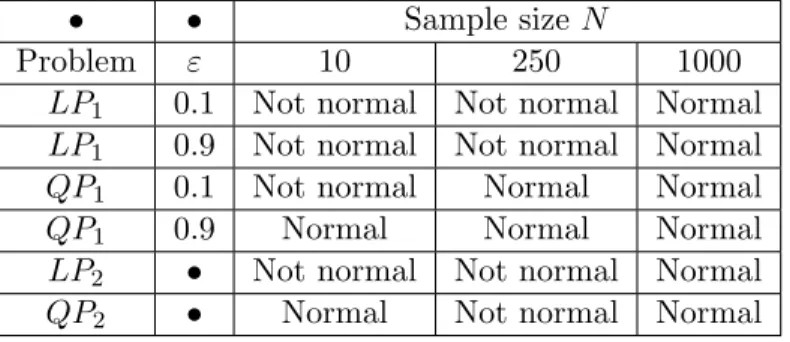
• • Sample size N

Problem " 10 250 1000

LP1 0.1 Not normal Not normal Normal

LP1 0.9 Not normal Not normal Normal

QP1 0.1 Not normal Normal Normal

QP1 0.9 Normal Normal Normal

LP2 • Not normal Not normal Normal

QP2 • Normal Not normal Normal

Table 1: Jarque Bera test for the SAA estimators of the optimal value of

(LP1), (LP2), (QP1), (QP2).

Introducing a quadratic penalization, we get problem (QP2):

Q2 = 8 < : minE[ ⇠Tx] + "0kxk22 E[( ⇠T_{x +E(⇠}T_x)) +] 2, x 0,Pn_i=1xi = 1,

with "0 = 10 3. Working analogously to the linear case, the corresponding SAA is

ˆ Q2,N = 8 > > > > > > > > > < > > > > > > > > > : min x 1 N N X i=1 ⇠T_i x + "0kxk22 x 0,Pn_i=1xi = 1 ti 0 8i 2 {1, . . . , N} ⇠_iTx _N1 PN_i=1⇠_iTx + ti 0 8i 2 {1, . . . , N} 1 N PN i=1ti  2. 6.2 Checking normality

Theorem 5.3 and Remark 5.1 tell us that the asymptotic distribution of the SAA estimators

of the optimal values of (QP1) and (QP2) is Gaussian and such will be the case for (LP1) and

(LP2) if they have unique primal and dual solutions. However, this theorem does not tell us the

value of the sample size above which the distribution of the SAA estimator of the optimal value can be well approximated by a Gaussian distribution. As a result, it is interesting to observe the impact of the sample size N on the distribution of the SAA estimator of the optimal value.

We will also be interested in measuring the impact of " in (LP1) and (QP1) on this distribution.

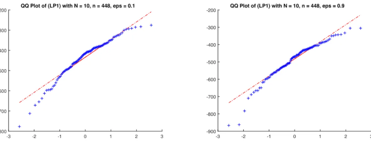
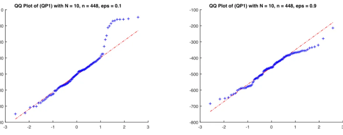
Therefore, in Figures 1-10, we represent the QQ-plots of the empirical distribution of the

optimal value of the SAA for (LP1), (LP2), (QP1), (QP2), versus the normal distribution with

the same mean and standard deviation. In these experiments, 100 samples of size N of ⇠ which generated 100 SAA problems were used.

To decide if the assumption of normality can be accepted or not for fixed (N, "), we used Jarque-Bera test, with 5 % of significance level. The results are reported in Table 1.