DOI: 10.1590/1808-057x201805080
Original Article
Asset growth and stock return: evidence in the Brazilian market
Márcio André Veras Machado1
https://orcid.org/0000-0003-2635-5240 Email: marciomachado@ccsa.ufpb.br
Robert William Faff2
Email: r.faff@business.uq.edu.au
1Universidade Federal da Paraíba, Centro de Ciências Sociais Aplicadas, Departamento de Administração, João Pessoa, PB, Brazil 2University of Queensland, Faculty of Business, Economics and Law, UQ Business School, Brisbane, QLD, Australia
Received on 01.30.2017 – Desk acceptance on 04.06.2017 – 4th version approved on 10.08.2017 – Ahead of print on 06.18.2018
Associate Editor: Fernanda Finotti Cordeiro Perobelli
ABSTRACT
Empirical evidence suggests that firms which have experienced fast growth, through increased external funding and by making capital investments and acquisitions, tend to show bad operating performance and lower stock returns, whereas firms that have experienced contraction, through divestiture, share repurchase and debt retirement, tend to show good operating performance and higher stock returns. So, this study aimed to analyze the relationship between asset growth and stock return in the Brazilian stock market, and it tested the hypothesis that asset growth is negatively related to future stock return. To do this, the methodology was divided into 3 steps: verifying 1) if asset growth anomaly exists; 2) if this relation may be explained by the investment friction hypothesis and/or by the limits-to-arbitrage hypothesis; and 3) if asset growth is a risk factor or mispricing. In addition, the analysis was carried out both at a portfolio level and an individual assets level. The sample included all the non-financial firms listed at B3 from June 1997 to June 2014. As for the main results, this study found that the asset growth effect exists, both at the portfolio level and the individual assets level, although it is sensitive to the proxy. About the effect’s materiality, this study concluded that the asset growth effect is not economically relevant, since it is not observed in big firms, regardless of the proxy used, a fact that makes it difficult to explore this effect. Another finding is that the asset growth effect may not be related to the limits-to-arbitrage hypothesis and to the financial constraint hypothesis; also, this effect may be considered a risk factor, suggesting that the investment effect documented in the Brazilian stock market may be explained by the rational asset pricing perspective. Therefore, capital market professionals should take into account the asset growth factor in asset pricing models for better investment risk assessment.
Keywords: anomalies, asset growth effect,investment effect, risk factors.
Correspondence address:
Márcio André Veras Machado
Universidade Federal da Paraíba, Centro de Ciências Sociais Aplicadas, Departamento de Administração Campus I – Via Expressa Padre Zé, 289 – CEP 58051-900
1. INTRODUCTION
Empirical evidence suggests that firms which have experienced fast growth, through increased external funding and by making capital investments and acquisitions, tend to show bad operating performance and lower stock returns, whereas firms that have experienced contraction, through divestiture, share repurchase and debt retirement, tend to show good operating performance and higher stock returns (Watanabe, Xu, Yao, & Yu, 2013; Yao, You, Zhang, & Chen, 2011; Cooper, Gulen, & Schill, 2008). This negative relation between investment and return is documented in the literature as investment effect or asset growth effect (Lipson, Mortal, & Schill, 2011).
One of the great discussions in the literature is if the negative relation existing between asset growth and stock return is an evidence of market inefficiency or if it may be regarded as a result of rational asset pricing (Watanabe et al., 2013). Hence, there are two approaches in the literature to explain the asset growth effect: one is rational and the other is behavioral (Cooper et al., 2008; Lipson et al., 2011; Lam & Wei, 2011).
Under the behavioral perspective, many explanations are based on mispricing, such as: the tendency of corporate managers to invest in negative net present value projects, due to information asymmetry and agency problems (Titman, Wei, & Xie, 2004; Myers, 1984; Myers & Majluf, 1984); market timing, i.e. managers adopt opportunistic behavior by issuing stocks when their value is high and buying stocks when their value is low (Baker & Wurgler, 2002); investors’ overreaction, overstating the asset’s past growth when valuing firms (Lakonishok, Shleifer, & Vishny, 1994); corporate earnings management (Teoh, Welch, & Wong, 1998), when managers tend to manipulate reported corporate earnings upward before obtaining external funding or before acquisition operations, as a way to gain favorable market-value valuation.
Explanations based on mispricing are related to the assumption that investors have the wrong reaction to public information available when they value stocks, thus lower stock returns of higher asset growth rates are a way for the market to correct that initial overreaction (Watanabe et al., 2013). According to Lam and Wei (2011), asset growth anomaly exists because investors fail or they are slow to include correct information about the firm’s investment into stock prices, a fact that causes mispricing; these authors explain that, in an optimal setting, when stocks are badly priced, investors might take the opportunity of riskless arbitrage and correct mispricing immediately. However, in a realistic market,
arbitrage is limited, risky, and costly; so, correcting mispricing takes longer.
From the rational asset pricing perspective, the explanation lies on the relationship between investment and expected return, where higher investments are bound to lower stock returns, according to the Q-theory of investment, which predicts that the marginal product of capital is a decreasing investment function (Li & Zhang, 2010; Lam & Wei, 2011;Chen, Novy-Marx, & Zhang, 2010; Lin & Zhang, 2013; Hou, Xue, & Zhang, 2015). This means that firms invest more when expected returns are lower and they invest less when expected return is higher, a fact evidencing a negative relation between investment and stock return.
The real options theory also explains the asset growth effect (Watanabe et al., 2013). It is based on the assumptions that real options are riskier than the assets in place. When firms make an investment, real options are made and converted into less risky assets in place. Therefore, firms making large investments tend to have lower risk and lower expected return in the future (Berk, Green, & Naik, 1999). So, there is a mix of growth option and assets in place, and this mix changes when firms decide to invest and grow. Considering the risk difference between new assets and assets in place, these changes may induce time-varying risks that may explain the asset growth effect (Li, Becker, & Rosenfeld, 2012).
Given the above, this study tested the hypothesis that asset growth is negatively related to future stock return. Hence, this paper aims to analyze the relationship between asset growth and stock return in the Brazilian stock market. To do this, the following steps were taken: investigate 1) if the asset growth effect exists in the Brazilian stock market; 2) investigate if the effect exists when return is adjusted to risk, according to traditional asset pricing models; 3) if asset growth influences stock return separately after controlling other determinants; 4) if the effect may be related to the financial constraints hypothesis and/or to the limits-to-arbitrage hypothesis; and, finally, 5) if asset growth is a risk factor to explain stock returns or mispricing. In this way, the asset growth risk factor and profitability (Novy-Marx, 2013) were included in the 3-factor model proposed by Fama and French (1993), making it a 5-factor model, according to Fama and French (2015).
a negative relation between asset growth and stock return outside the United States of America (USA). So, we may infer whether the behavior pattern documented in the USA is due to chance or to data snooping, according to Lo and Mackinlay (1990). Despite the large number of studies examining the relationship between asset growth and stock return, both in the USA (Cooper et al., 2008; Fama & French, 2008; Lipson et al., 2011), and in international markets (Yao et al., 2011; Li et al., 2012; Watanabe et al., 2013), only one paper has examined the asset growth effect in Brazil (Ribeiro, 2010).
The studies by Li et al. (2012), Watanabe et al. (2013), and Ribeiro (2010) are those more closely related to this research. However, Li et al. (2012) analyzed only developed countries, while Watanabe et al. (2013) also included developing countries in their sample (including Brazil), although the latter addressed only common shares.
Ribeiro (2010) highlights that a limitation of her study was lack of data, since they analyzed only 26 Brazilian firms. In turn, this research analyzed on average 168 firms per year, representing on average 48% of the firms in the Brazilian market, as well as 74% of market capitalization and 17 years of analysis. In addition, this article contributes to the literature as it not only analyzes the relation between asset growth and stock returns, but also verifies whether asset growth anomaly may be explained by the investment friction hypothesis and/or by the limits-to-arbitrage hypothesis, as well as if asset growth is a risk factor or mispricing, which were not observed in Ribeiro (2010). Finally, more than addressing asset growth anomaly, this paper also analyzed its economic relevance, as highlighted by Fama and French (2008).
Brazil has been chosen because this is a country with
peculiar characteristics that may make the market react positively to investing in assets. Unlike the USA, where the capital market is well-developed, Brazil depends greatly on bank-based financial systems to fund its activities. Therefore, the banking system is a major source for funding asset growth; subsidized funding lines by official sources allow firms to borrow resources at a low cost. For instance, funding obtained from the Brazilian National Bank for Economic and Social Development (BNDES), one of the country’s most important official funding sources, is accountable for high volume and low cost.
Also, there is empirical evidence that the existing conflict of interest between managers and shareholders is the asset growth effect’s source in the USA (Cooper et at., 2008). Nevertheless, in Brazil, this conflict between managers and shareholders happens less frequently than in the USA, where firms’ capital is diversified. Most Brazilian firms have a controlling shareholder who owns most of the common voting stocks, so he controls the firm. Hence, the biggest conflict is between majority and minority shareholders. Let us add to this fact the existence of common voting stocks and a high issuance of preferred non-voting shares; thus, considering that the governance structure in Brazil is different from that in the USA, since property is highly concentrated in the families and the government’s hands, as well as a large number of preferred stocks in circulation, this study becomes even more important.
This paper is structured into four sections. The second section introduces previous studies and the main empirical evidence; the third section introduces the methodology; and the fourth section presents our results. Finally, the reader is provided with our final remarks.
2. PREVIOUS STUDIES
Xing (2008) and Cooper et al. (2008) were some of the first to analyze the relationship between investment and expected return in the USA. Xing (2008) analyzed, using the regression proposed by Fama and MacBeth (1973), 43,277 firms/year from 1964 to 2003 and interpreted the value effect, by means of Q-theory of investment’s implications, through the capital investment variation, as well as the capital investment divided by the total net asset, as a proxy for asset growth. As their main results, the authors found a negative relation between investment and stock return, according to the assumptions of the Q-theory of investment; they also found that the investment effect is priced and this has the same information level as the book-to-market (BM) ratio in the 3-factor model proposed by
Fama and French (1993). Cooper et al. (2008), using the total asset variation as a proxy and the same econometric method, within the same time period, confirmed the results of Xing (2008).
Just like Xing (2008) and Cooper et al. (2008), Lam and Wei (2011) found, through the regression proposed by Fama and MacBeth (1973), a negative and significant relation between stock returns and asset growth in U.S. firms from 1971 to 2009. Also, the authors analyze what better explained asset growth anomaly: the limits-to-arbitrage hypothesis, the investment friction hypothesis, or both of them. The authors concluded that both hypotheses were important, thus complementary in order to explain such anomaly. However, by using value-weighted returns, the support of both hypotheses was weaker. Finally, the authors observed that volatility was the only proxy with a significant effect on asset growth anomaly. Moreover, firm age was the only investment friction proxy showing a satisfactory effect. So, unlike Li and Zhang (2010), Lam and Wei (2011) found that both the investment friction hypothesis and limits-to-arbitrage contribute to explain asset growth anomaly.
Lipson et al. (2011) analyzed, through the regression proposed by Fama and MacBeth (1973), the relation between asset growth and stock returns by using seven proxies for asset growth in the USA, from 1968 to 2006. As main results, they found a significant negative relation between stock returns and asset growth, regardless of the proxy used. However, the effect was better captured when total asset was used, since this absorbs the effect of all other proxies. In addition, the authors observed that the effect is economically relevant and it is not restricted to small-sized firms, as stated by Fama and French (2008). Just like Li and Zhang (2010), Lipson et al. (2011) observed that the cost of arbitrage was a necessary condition to the asset growth effect; thus, it is related to mispricing.
Gray and Johnson (2011) and Bettman, Kosev and Sault (2011) analyzed the relation between asset growth and stock returns in Australian firms. Gray and Johnson (2011) analyzed, through the regression proposed by Fama and MacBeth (1973), an average of 1,248 firms/ year from 1981 to 2006, and found a significant negative relation, even after including other traditionally known determinants, such as BM ratio, size, and momentum. Like Gray and Johnson (2011), Bettman et al. (2011), from 1998 to 2008, found the asset growth effect only when return was equally-weighted. When the analysis was conducted as an individual asset function, by analyzing the cross-sectional relation between asset growth and stock returns, although it showed the expected sign, the coefficient was not significant, in any of the specifications used.
Yao et al. (2011), Li et al. (2012), and Watanabe et al. (2013) addressed the relation between asset growth and stock returns in international markets. Yao et al. (2011) analyzed through panel data the relation between asset
growth and stock returns in 9 Asian countries, from 1981 to 2007, resorting to total asset variation, as well as the variation of their components and that of the total liability components, as proxy for asset growth. As main results, the authors found a negative relation between asset growth and stock returns; however, it was a weaker relation than that found in the USA. As for the asset growth effect’s magnitude in Asia, when compared to the USA, the authors found that the homogeneity of asset growth, as well as the total asset components, may alleviate the asset growth effect.
Li et al. (2012) analyzed, through the regression proposed by Fama and MacBeth (1973), the relation between asset growth and stock returns in 23 developed countries, from 1963 to 2008, using 7 proxies for asset growth. As main results, the authors found a negative relation between asset growth and stock returns, regardless of the proxy and normalization used, even after including control variables. However, with value-weighted findings, the relation showed to be significant only when total asset variation was used as a proxy.
Watanabe et al. (2013) analyzed, through panel data, the relation between asset growth and stock return in 43 countries, from 1982 to 2010, using total asset variation as an asset growth proxy. The final sample comprised 291,725 firms/year. Their overall major results show that the asset growth effect was found in international markets, even after including other return determinants, such as BM ratio, size, and momentum, thus evidencing that the effect exists outside the USA. Premium ranged from -11% to 11% per year (equally-weighted return) and from -14% to 15% per year (value-weighted return), with positive spreads in 30 countries and negative spreads in 13 countries. In Brazil, specifically, they found a spread of -3.24% per year, which is not statistically significant. Also, the authors analyzed possible economic causes for the asset growth effect, considering a significant debate in the literature: if asset growth is an evidence of market inefficiency or if it may be understood as a result of rational asset pricing. So, the authors found that the asset growth effect was more noticeable in developed markets, i.e. markets where stocks are more efficiently priced. On the other hand, characteristics such as limits to arbitrage, investor protection, and accounting quality had a limited power to explain the asset growth effect’s variation. Therefore, the authors conclude that the asset growth effect is rather related to the optimal investment theory than mispricing forms, such as market timing and overinvestment.
growth and stock returns for 26 firms belonging to the Ibovespa index, from 2000 to 2009, using total asset as proxy for asset growth, and she did not find any evidence to support this relation. According to the author, the lack
of a relation may be associated to the existence of official funding sources, which allows big conglomerates to raise funds at a low cost, preventing investment in total assets in Brazil to be considered as negative by investors.
3. METHODOLOGY
3.1. Data
Data used in this study were collected from the database Economatica, largely used in Brazil, which provides accounting and market information on the firms listed at B3 (‘Brasil, Bolsa, Balcão’). Data include firms that are both active and inactive in the capital market, to avoid survivor bias. The sample’s period was from June 1, 1997, to June 30, 2014. The year 1997 was chosen because the operationalization of some variables resorts to data related to two previous years, which culminates in using data from 1995. Data prior to the year 1995 in Brazil are affected by high inflation rates and lack of currency standardization. Finally, when the company under analysis had more than one stock class and type, the most liquid stock was chosen, based on the mean volume traded within the last 12 months.
These firms were excluded from the analysis: a) financial firms, since Fama and French (1993) pointed out that a high BM ratio does not mean the same for non-financial and non-financial firms; the latter’s ratio is influenced by their high leverage degree; b) firms that did not have market value set on December 31 and June 30 each year, as these values serve to compute the BM ratio and firm
size; c) firms that had negative equity on December 31 each year, as it affects the BM ratio; d) firms that did not have monthly quotations for 24 consecutive months, 12 months prior to portfolio formation and 12 months after that, considering that this procedure reduces the influence of small-sized and young firms on the results (Anderson & Garcia-Feijó, 2006); and e) firms that did not have information concerning the accounting data used. Per year, data on 153 stocks (38% of the population), on average, were analyzed. The year 2003 had a minimum of 78 stocks (21% of the population) and 2012 had a maximum of 217 stocks (56% of the population). This sample’s size is satisfactory, when compared to other studies, mainly international studies using Brazilian stock data. Machado and Medeiros (2011) and Walkshäusl and Lobe (2014) analyzed, on average, 149 and 178 stocks per year, respectively. As for market capitalization, within the period from 1997 to 2013, the sample corresponded to a minimum of 54% in 1998 and a maximum of 94% in 2010. In this study sample, 48% of the firms represent 85% of market capitalization within the period analyzed.
Considering that the best way to measure asset growth has not been well-established, 5 proxies were used, based on previous studies:
a) Xing (2008), who determines that penditure growth rate(Equation 1):
b) Cooper et al. (2008), who define asset growth as a total asset growth rate (Equation 2):
c) Fama and French (2008), who use an asset growth rate adjusted to the stocks issued to measure the asset growth (Equation 3):
d) Lyandres, Sun and Zhang (2008), who use annual changes in inventories plus the annual changes of fixed assets divided by the two-lag total asset to measure asset growth (Equation 4):
1
2
3 t-1
t-2
capital expenditures 1 capital expenditures
XING =
t-1
t-2 Total Asset
1 Total Asset
CGS =
t-1
t-2
Total Asset
1
Total Asset Net Stock Issues from t-2 to t-1
FF =
3.2. Research Design
In order to analyze the relation between asset growth and stock return, the methodology was divided into 3 steps: verifying 1) if asset growth anomaly exists; 2) if this relation may be explained by the investment friction hypothesis and/or by the limits-to-arbitrage hypothesis; and 3) if asset growth is a risk factor or mispricing. To do this, the analysis was conducted both at a portfolio level and an individual stock level.
3.2.1. Verifying if asset growth anomaly exists.
At first, the analysis was conducted at the portfolio level. Therefore, by the end of June of each year t, stocks were arranged into ascending order according to each asset growth proxy; then, they were sorted into 5 portfolios based on quintile breakpoints. From July of year t to June of year t+1, the average monthly value-weighted return for each portfolio was calculated. The portfolios were rebalanced annually. Portfolios were rebalanced by the end of June of each year to guarantee that data on the financial statements concerning the previous calendar year have already been published and absorbed by the
market, thus preventing look-ahead bias(Machado & Medeiros, 2011).
Finally, to analyze if the asset growth effect has been restricted only to small firms, another issue was addressed: the behavior of average returns for portfolios formed from the combination of 3 size groups and 5 asset growth groups (3 x 5). Size groups were defined by classifying firms into 3 groups (small-sized, medium-sized, and big), through the firm’s market value tertile (30%, 40%, and 30%) in June of each year.
If there is a tendency for excess returns across the 5 portfolios, then the effect exists. So, in order to conclude that the asset growth effect exists, the returns for low portfolios must be higher than the returns for high portfolios.
Also, the study investigated if the effect exists when the return is adjusted to the 3-factor and 5-factor models (Equations 6 and 8) proposed by Fama and French (1993, 2015) and to the 4-factor model proposed by Carhart (1997) (Equation 7); i.e. the study evaluated the aforementioned models’ ability to explain asset growth anomaly.
e) Polk and Sapienza (2009), who define asset growth as an index obtained by dividing capital expenditures by net fixed assets (Equation 5):
where: Rp,t is the portfolio return in month t; Rf,t is the risk-free rate in month t, by adopting the SELIC rate as a proxy; Rp,t– Rf,t is the excess portfolio return; Rm,t
is the market return in month t; Rm,t – Rf,t is the market risk premium; SMBt, HMLt, RMWt, CMAt, WMLt are, respectively, size, BM ratio, profitability, investment, and
momentum factors, all of them in month t; α, β, s, h, w, r, and c are the regressions’ estimated coefficients; and εt is the random error term.
To obtain the risk factors of the 3-factor, 4-factor, and 5-factor models, stocks were classified into 2 x 2, 2 x 3 x 2 and 2 x 2 x 2 x 2 sorts, with the following interactions,
4
5
6
7
8
t-1 t-2 t-1 t-2
t-2
Inventories Inventories +Fixed Asset Fixed Asset
1 Total Asset
LSZ =
t-1
t-2 t-2
capital expenditures
1
Fixed Asset depreciation
PS =
p,t - R = f,t i[ ( m,t)-R ]+s SMB +h HML + f,t
t
t tE R α+ β E R ε
p,t f,t m,t f,t
( )-R i ( )-R +s(SMB)t ( )t ( )t t
E R = α+ β E R +h HML + w WML +ε
p,t f,t m,t f,t
( )-R i ( )-R +s(SMB)t ( )t ( )t ( )t t
respectively: size and BM ratio; size, BM ratio, and momentum; and size, BM ratio, profitability, and asset growth. The market factor is obtained by the difference between the average monthly value-weighted return of all sample stocks and the risk-free rate, with the SELIC rate as a proxy.
The estimation of equations 6, 7, and 8 must provide evidence on the risk factors’ ability to capture asset growth anomaly. To do this, alpha values for the models are estimated in the 15 portfolios created from size and asset growth (3 x 5). When alpha values are not significant, we may claim there is no abnormal return after adjusting to market, size, BM ratio, profitability, and investment factors.Otherwise, we may state that the strategy of purchasing stocks with lower asset growth leads to statistically significant risk-adjusted abnormal returns.
The analysis by portfolios has one advantage: it does not have to take up a functional mode for the relation between return and investment; however, it has one disadvantage: the ability to control other factors is limited. Besides, these variables used to build portfolios and calculate spreads may not be associated with average returns. Therefore, there is a need to examine the relation between asset growth and individual stock returns to determine whether the asset growth variable has a different influence on cross-section returns after controlling other return determinants. To do this, the methodology proposed by Fama and MacBeth (1973) has been adopted for estimating the coefficients of interest, according to Equation 9. Estimating this equation provides evidence on the sign of the coefficient for the asset growth variable, which must be negative, in order to detect the existence of asset growth anomaly.
where Rt is the annual stock return from July of year t
to June of year t+1; AG is asset growth, according to the proxy used;MV is the natural logarithm of the firm’s market value in June of year t; BM ratio refers to book equity divided by market equity in December of year t-1; MOM is the accumulated stock return from July of year
t-1 to May of year t; andE/A is the net profit divided by total asset.
3.2.2. Verifying if asset growth anomaly may be explained by the investment friction hypothesis and/or by the limits-to-arbitrage hypothesis.
According to Li and Zhang (2010), the relation between stock return and investment is steeper in firms with high investment friction, considering that, with frictions, investments lead to elevated costs, making investments less elastic to changes in the discount rate than when such frictions are absent. Therefore, the higher the investment costs, the less elastic the investments in response to variations in the discount rates. Likewise, a change at the investment level implies an even bigger change in the discount rate.
Given all the above, the relation between stock return and investment should be steeper in firms with high investment friction than in firms with low investment friction. To test this assumption, 2 proxies for financial constraints were used: payout ratio and total asset. Therefore, the firms included in the sample were split into tertiles, according to each proxy. Next, Equation 9 was
estimated for extreme subsample, in order to investigate whether there were differences in the coefficients for the asset growth variable.
Firms with low payout ratio and low total asset are expected to have more financial constraints than firms with a high payout ratio and high total asset. Therefore, if the asset growth effect is consistent with the financial constraints hypothesis and with the Q-theory of investment, the coefficient for the AG variable in Equation 9 is higher in the more constrained subsample than in the less constrained subsample.
If stocks are mispriced, then opportunities for profitable investments attract rational investors, who should correct mispricing by means of arbitrage. In an optimal setting, where opportunities for arbitrage are riskless and costless, prices should reflect all the information available, and mispricing, if there is any, should be immediately corrected. However, in a realistic market, where arbitrage is costly and risky, arbitrage is limited, considering that costs may exceed the benefits (Lam & Wei, 2011; Lipson et al. 2011).
Considering the limits-to-arbitrage as an alternative to the Q-theory of investment, attention was paid to trading friction, as well as to investment friction. Therefore, the relation between stock return and investment should be steeper in firms with high limits-to-arbitrage than in firms with low limits-to-arbitrage (Li & Zhang, 2010). To test this assumption, 2 limits-to-arbitrage proxies were used: volatility, measured by the standard deviation of
9
2,t 3,t 4,t 5,t
AG+ MV+ BM+ MOM+ E/A
t 1,t t
returns, and liquidity, measured by the average volume traded within the last 12 months. The sampled firms were separated into tertiles, according to each proxy. Firms with high volatility and low trade volume are expected to have higher limits-to-arbitrage. Likewise, the AG variable coefficient in Equation 9 is expected to be higher in the subsample with higher limits-to-arbitrage.
3.2.3 Verifying if asset growth is a risk factor or mispricing.
At last, in order to test if asset growth is a priced risk factor, 2 risk factors – profitability and investment – were
added to the 3-factor model proposed by Fama and French (1993) to make up the 5-factor model proposed by Fama and French (2015), according to Equation 8.
The 2-stage cross-sectional regression methodology was used; the first stage estimated the regression beta values and the second stage estimated the factor risk premiums. This method provides a well-specified test for the hypothesis that a risk factor explains variation in expected returns, just as a significant risk premium is seen as an evidence that the risk factor is priced (Core, Guay, & Verdi, 2008). So, the portfolio beta values were estimated through Equation 10.
where: Rp,t is the return for the portfolio built from size and on BM ratio (3 x 5) in month t; Rf,t is the risk-free rate in month t; Rm,t is the market return in month t; SMBt,
HMLt, RMWtand AGt are, respectively, premiums for size, BM ratio, profitability, and asset growth factors in
month t; and εt is the random error term.
In the second stage, a single cross-sectional regression for the average excess returns was estimated on the estimated beta values of Equation 10. Thus, factor risk premiums were estimated through Equation 11.
where: Rp - Rf is average excess return for the period analyzed; are the estimated parameters in the first stage; λ1,λ2,λ3,λ4,and λ5 are the factor risk premiums, with special interest in the coefficient λ5; in order to turn asset growth into a priced risk factor, this parameter must be positive and significant.
Since independent variables in Equation 11 are regressors estimated through Equation 10, a mechanism must be used to correct standard error for the factor risk premium (Core et al., 2008; Gray & Johnson, 2011).
The mechanism adopted was the method proposed by Shanken (1992), because the standard error computed for Fama and MacBeth (1973) may be underestimated, due to the fact that the second-stage independent variable is estimated in the first-stage regression (Core et al., 2008). Therefore, standard error was corrected through the factor , where is the covariance matrix for SMB, HML, RMW, and AG factors and is the matrix for estimated parameters.
10
11
p,t f,t , m,t f,t P,SMB t , , , t
E(R )-R = + P mktE(R )-R + (SMB) p HLML(HML)tp RMW(RMW)tp AG(AG)t
p,SMB
ˆ
ˆ
ˆ
ˆ
ˆ
p f 0 1 P,mkt 2 3 p,HLML 4 p,RMW 5 p,AG t
R
R = λ + λ β
+ λ β
+ λ β
+ λ β
+ λ β
+ε
*
p,
4. RESULTS
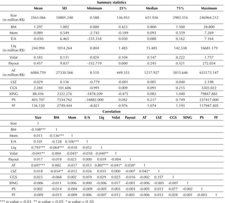
Table 1 displays the average value and the correlation between the variables used in this study, within the period from 1995 to 2014. The firms included in the sample have, on average, a market value of R$ 3.563 million and total assets worth R$ 6.084 million, BM ratio of 1.297, and
profitability of -0.03. Besides, these firms have an average trading volume of R$ 244 million and a payout ratio of 0.457. As for asset growth proxies, their average values range from 0.029 (LSZ) to 403 (PS).
Table 1
Summary Statistics and Correlation
Summary statistics
Mean SD Minimum 25% Median 75% Maximum
Size
(in million R$) 3563.066 10801.240 0.588 136.953 651.936 2983.516 246964.212
BM 1.297 1.802 0.000 0.423 0.800 1.500 28.800
Mom 0.089 0.549 -2.742 -0.189 0.093 0.359 7.269
E/A -0.030 6.465 -335.318 0.030 0.088 0.162 7.164
Liq
(in million R$) 244.994 1014.264 0.004 1.483 15.485 142.538 16681.179
Volat 0.183 0.131 0.024 0.104 0.147 0.222 1.757
Payout 0.457 9.837 -332.719 0.000 0.245 0.521 272.034
AT
(in million R$) 6084.759 27330.566 8.510 449.353 1217.927 3815.646 633173.147
LSZ 0.029 0.136 -0.779 -0.001 0.001 0.040 2.198
CGS 2.284 101.606 -0.991 0.009 0.091 0.215 5303.022
XING 88.436 2322.276 -1878.209 -0.475 0.083 1.040 79847.882
PS 403.707 7534.762 -34882.000 0.042 0.217 0.749 257417.000
FF 136.120 2749.444 -8.821 0.976 1.074 1.193 117947.405
Correlation
Size BM Mom E/A Liq Volat Payout AT LSZ CGS XING PS FF
Size 1
BM -0.108*** 1
Mom 0.011 -0.136*** 1
E/A 0.101 -0.128 0.106*** 1 Liq 0.793*** -0.064*** -0.018 0.052 1 Volat -0.041** 0.004 -0.045* -0.018 -0.040** 1 Payout 0.017 -0.018 0.023 0.000 0.039 -0.004 1
AT 0.697*** 0.002 -0.017 0.015 0.807*** -0.041* 0.038* 1 LSZ 0.018 -0.034** -0.012 0.026 0.035 0.000 -0.007 0.042* 1 CGS 0.023 -0.068 0.002 0.059 0.029 0.025 -0.016 -0.002 0.357 1 XING -0.006 -0.011 0.006 0.000 -0.006 0.017 -0.001 -0.006 -0.005 -0.007 1
PS 0.002 -0.014 -0.004 -0.009 -0.005 0.003 -0.003 -0.005 0.012 0.077 -0.002 1 FF -0.009 -0.015 -0.009 0.006 -0.007 0.012 0.003 -0.006 0.012 0.028 -0.001 -0.003 1
*** p value < 0.01, ** p value < 0.05, * p value < 0.10.
Regarding correlations, the correlation coefficient between size and asset growth ranges from -0.009 (FF) to 0.023 (CGS). The BM ratio is negatively correlated with all asset growth proxies, corroborating previous studies (Anderson & Garcia-Feijó, 2006; Xing, 2008; Lipson et al., 2011). Also, the asset growth proxies related to capital expenditures (XING and PS), as well as the asset growth proxies based on asset growth (LSZ and CGS), are correlates, and this is the strongest correlation between the asset growth proxies.
4.1. Portfolio Analysis
Table 2 displays the average returns for portfolios built from asset growth. By using XING as a proxy, the asset growth effect is not found, since the monthly average return for the portfolio built from stocks of firms with
lower asset growth is lower than the monthly average return for the portfolio formed by stocks of firms with higher asset growth, although spread was not statistically significant. These findings contradict the results provided by Cooper et al. (2008), Xing (2008), Fama and French (2008), and Lipson et al. (2011), considering that these authors found that portfolios built from low investment stocks had higher returns than the portfolios formed by high investment stocks.
However, by using the CGS, FF, LSZ and PS measurements as an asset growth proxy, there is evidence of the asset growth effect. Nevertheless, spread was statistically significant only for the LSZ measurement. The 0.9% monthly spread (11.35% per year) is close to that provided by previous studies (Lam & Wei, 2011; Lipson et al., 2011; Li et al., 2012).
Table 2
Returns for portfolios built from asset growth
High AG Q2 Q3 Q4 Low AG Spread
(Low AG - High AG)
XING 0.015 0.013 0.013 0.013 0.013 -0.002
CGS 0.013 0.016 0.010 0.012 0.017 0.003
FF 0.013 0.018 0.011 0.010 0.014 0.001
LSZ 0.012 0.012 0.013 0.010 0.020 0.009*
PS 0.012 0.013 0.018 0.014 0.014 0.003
*** p value < 0.01, ** p value < 0.05, * p value < 0.10.
Source: Prepared by the authors.
Next, the analysis was conducted through firm size, in order to check if the asset growth effectwas specific to small firms, as stated by Fama and French (2008), or if it was observed in several size groups, mainly among big firms, which was the primary focus of this analysis. Addressing the asset growth effect in the various size groups has two implications: one of them is practical and the other is economic. From the practical perspective, if the effect exists only in small firms, the anomaly is not likely to be explored, due to the high transaction costs of these stocks. From the economic perspective, it is worth knowing if the effect is observed throughout the market or if it is limited to illiquid stocks, those which are more
difficult to be explored (Fama & French, 2008).
Table 3
Returns for the portfolios built from asset growth and size
High AG Q2 Q3 Q4 Low AG L-H
Big size
LSZ 0.014** 0.009 0.015** 0.008 0.0208* 0.006
CGS 0.011* 0.013** 0.017** 0.006 0.016*** 0.005
XING 0.012 0.014** 0.014** 0.013** 0.011 -0.001
PS 0.014** 0.012* 0.014** 0.014** 0.013** -0.001
FF 0.009 0.017*** 0.012* 0.011 0.011* 0.002
Medium size
LSZ 0.011* 0.009 0.018* 0.013** 0.021* 0.010*
CGS 0.007 0.021*** 0.010 0.013** 0.018*** 0.011***
XING 0.012* 0.015** 0.008 0.016*** 0.017*** 0.005
PS 0.007 0.018*** 0.012** 0.011* 0.018*** 0.011**
FF 0.012* 0.016** 0.014** 0.015*** 0.011 -0.001
Small size
LSZ 0.010 0.014** 0.008 0.021** 0.011 0.001
CGS 0.010 0.008 0.011* 0.019*** 0.009 -0.002
XING 0.023*** 0.010* 0.002 0.010 0.014 -0.009
PS 0.008 0.013** 0.014** 0.010 0.014 0.005
FF 0.017*** 0.006 0.019*** 0.010* 0.001 -0.017*
*** p value < 0.01, ** p value < 0.05, * p value < 0.10.
Source: Prepared by the authors.
The study also investigated the existence of the asset growth effectafter adjusting return to risk, according to the 3-factor and 5-factor models proposed by Fama and French (1993, 2005) and to the 4-factor model proposed by Carhart (1997). The alpha values were estimated for the Small-Sized, Medium-Sized, and Big portfolios, as well
as for the portfolio with all stocks included in the sample without sorting by size. As return is adjusted to risk, the results evidenced in Table 4 ratify the results displayed in tables 2 and 3: spread is significant only when LSZ is used as a proxy and spreads are not significant in big firms regardless of the proxy and the pricing model used.
Table 4
Spreads of returns adjusted to risk
Proxy 3-factor 4-factor 5-factor
All
XING 0.000 0.000 -0.002
CGS 0.005 0.006 0.007*
FF 0.003 0.006 0.006
LSZ 0.008* 0.009* 0.008*
PS 0.008 0.007 0.007
Big size
XING 0.006 0.003 0.004
CGS 0.004 0.005 0.007
FF 0.002 0.005 0.005
LSZ 0.009 0.009 0.009
Proxy 3-factor 4-factor 5-factor Medium size
XING 0.008 0.004 0.007
CGS 0.011*** 0.009** 0.013***
FF -0.002 -0.002 0.000
LSZ 0.012** 0.009* 0.011**
PS 0.015* 0.010 0.016*
Small size
XING -0.004 -0.008 -0.006
CGS 0.001 -0.006 0.006
FF -0.009 -0.013*** -0.007
LSZ 0.000 -0.005 0.000
PS 0.009 0.007 0.008
*** p value < 0.01, ** p value < 0.05, * p value < 0.10.
Source: Prepared by the authors.
4.2. Individual Stocks Analysis
This study examined the relationship between asset growth and returns for individual assets, in order to investigate if the asset growth variable has a different influence on cross-sectional returns after controlling for other return determinants. Table 5 displays the estimated coefficients, according to Equation 9. Panel A concerns
regressions for all firms, whereas Panels B, C, and D, respectively, refer to regressions conducted for small-sized, medium-sized, and big firms. Size groups are defined through the classification of firms into 3 groups (small-sized, medium-(small-sized, and big), through the firm’s market value tertile (30%, 40% and 30%) in June of each year, rebalanced annually.
Table 5
Fama-MacBeth regressions for return with asset growth and other control variables
Panel A – All firms
1 2 3 4 5 6
Intercept 0.3630** 0.3498** 0.3731** 0.3649** 0.3646** 0.3760**
VM -0.0223** -0.0206** -0.0227** -0.0218** -0.0222** -0.0240**
BM -0.1036*** -0.1059*** -0.1057*** -0.1068*** -0.0942*** -0.1003***
MOM 0.3527*** 0.3561*** 0.3537*** 0.3515*** 0.3723*** 0.3473***
E/A 0.0813 0.0934 0.0733 0.0850 0.0664 0.1157
CGS -0.0714**
FF -0.0023
LSZ -0.3047***
PS -0.0001
XING 0.0004
R2 0.2901 0.2970 0.2947 0.2966 0.3023 0.2902
Panel B – Small-sized firms
Intercept 0.3285 0.296 0.2138 0.3405 0.3537 0.3933***
VM -0.0176 -0.0130 -0.0149 -0.0182 -0.0179 -0.0249
BM -0.0869** -0.0898** -0.1059*** -0.0906** -0.0804** -0.0744*
MOM 0.4033*** 0.4198*** 0.3989*** 0.4192*** 0.4723*** 0.3968***
E/A 0.0417 0.0619 -0.0185 0.0196 -0.1420 0.0348
Table 4
1 2 3 4 5 6
CGS -0.1482
FF 0.1040
LSZ -0.2752
PS -0.0016
XING -0.0003
R2 0.3778 0.4036 0.3944 0.4009 0.4271 0.3913
Panel C – Medium-sized firms
Intercept 0.4733** 0.4132** 0.4945** 0.4968** 0.3983 0.4357***
VM -0.0335*** -0.0280** -0.0355*** -0.0350** -0.0246 -0.0305*
BM -0.1428*** -0.1507*** -0.1441*** -0.1476*** -0.1470*** -0.1243***
MOM 0.3620*** 0.3475*** 0.3556*** 0.3566*** 0.3638*** 0.3709***
E/A 0.0072 0.0400 -0.0002 -0.0123 -0.1230 0.1130
CGS -0.1339*
FF 0.0031
LSZ -0.3353**
PS 0.0004
XING 0.0009
R2 0.3306 0.3557 0.3449 0.3474 0.369 0.3552
Panel D – Big firms
Intercept 0.1307 0.2215 0.0485 0.1537 0.0361 0.1942
VM -0.0027 -0.0077 0.0027 -0.0023 0.0036 -0.0086
BM -0.1082* -0.1170* -0.1176* -0.1170* -0.1019* -0.0977*
MOM 0.3907*** 0.3913*** 0.3728*** 0.4112*** 0.4482*** 0.3856**
E/A -0.4510* -0.4737 -0.4675* -0.5432 -0.4967* -0.3249*
CGS -0.1497
FF 0.0019
LSZ -0.5966
PS -0.0010
XING -0.0042
R2 0.3995 0.3893 0.3826 0.3811 0.4071 0.3960
*** p value < 0.01, ** p value < 0.05, * p value < 0.10.
Source: Prepared by the authors.
Panel A displayed in Table 5 shows that for all models, market value, BM ratio, and momentum influence on determining returns, whereas profitability does not have statistical significance. Also, except for BM ratio, all variables have the expected sign. The BM ratio signal turned out the opposite of what was expected, a fact which ratifies the previous empirical evidence in Brazil (Machado & Medeiros, 2011, 2012).
As for the asset growth variable – the main variable of interest –, as Xing is used as a proxy, apart from not being statistically significant, the signal is opposite to that expected. Moreover, when LSZ and CGS are used as proxies, there is a statistically significant and negative relation, as expected. These results ratify those displayed in
Table 2 and suggest that the asset growth effect is sensitive to the proxy used and that the LSZ proxy is the most appropriate (more consistent) to explain stock returns in Brazil. Perhaps, in Brazil the correlation between returns and inventories and fixed assets are stronger than the correlation between returns and the other balance items. After obtaining these results, this study focused on LSZ as asset growth proxy.
Regarding the effect’s materiality, the results provided by Panel D in Table 5 ratify the results provided by Fama and French (2008), as well as those displayed in Table 3, thus suggesting that the asset growth effect is not economically relevant, since the effect is not observed in big firms, regardless of the proxy used. Hence, just as
Table 5
observed in portfolio analysis (Table 3), there is evidence that the asset growth effect displayed in Table 5 is specific to medium-size firms.
4.3. What Explains the Asset Growth Effect?
This section addresses the relationship between stock returns and asset growth may be explained by the financial friction hypothesis or by the limits-to-arbitrage hypothesis. So, two proxies for financial constraints were used (payout ratio and total asset) and two proxies for limits-to-arbitrage (volatility, measured by the standard deviation of returns, and liquidity, measured by the average volume traded within the last 12 months). The relation between stock returns and investment is expected
to be more pronounced in firms with high investment friction and high limits-to-arbitrage.
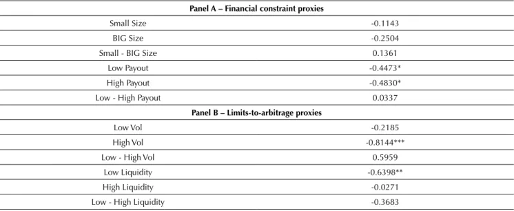
Table 6 displays the estimated coefficients for the asset growth variable at the extreme subsamples split by the financial constraints and limits-to-arbitrage proxies. Using the payout ratio as a financial constraint proxy, the coefficients are very close: -0.4473 (p value < 0.10) at the lowest tertile, and -0.4830 (p value < 0.10) at the highest tertile, a difference of -0.0337, although not statistically significant. By using total asset as a proxy, the results are similar, and there is no significant difference between the extreme subsamples. These results may indicate failure in the proxies used to capture financial constraints, as noticed by Farre-Mensa and Ljungqvist (2015).
Table 6
Coefficients of the asset growth variable in the sub-samples divided by the financial constraint and limits-to-arbitrage proxies
Panel A – Financial constraint proxies
Small Size -0.1143
BIG Size -0.2504
Small - BIG Size 0.1361
Low Payout -0.4473*
High Payout -0.4830*
Low - High Payout 0.0337
Panel B – Limits-to-arbitrage proxies
Low Vol -0.2185
High Vol -0.8144***
Low - High Vol 0.5959
Low Liquidity -0.6398**
High Liquidity -0.0271
Low - High Liquidity -0.3683
*** p value < 0.01, ** p value < 0.05, * p value < 0.10.
Source: Prepared by the authors.
Considering that the financial constraint hypothesis has not been consistent, the limits-to-arbitrage hypothesis was investigated. By using volatility as a proxy, the coefficient for the asset growth variable in the highest tertile is -0.8144 (p value < 0.01), whereas in the lowest tertile it is -0.2185, a difference of -0.5959 between the extreme subsamples, albeit not statistically significant. Results are similar (the difference is not significant) when using the traded volume as a proxy. These results suggest that arbitrage in Brazil is limited and that its costs may exceed the benefits (Lam & Wei, 2011; Lipson et al. 2011).
Therefore, according to the results displayed in Table 6, the asset growth effect has not been consistent with the financial friction hypothesis and the Q-theory of
investment, or with the limits-to-arbitrage hypothesis.
4.2. Asset Growth: Risk Factor or Mispricing?
This section investigates if the asset growth effect displayed in tables 2 and 4, when LSZ is used as a proxy, it is a risk factor or mispricing. To do this, the 2-stage cross-sectional regression methodology was used: in the first stage, the risk factor beta values were estimated in a time series; in the second stage, the risk factor premiums were estimated through cross-sectional regression. Table 6 displays the estimated parameters of stages 1 (Equation 10) and 2 (Equation 11).
growth effect. Table 7 shows that the asset growth factor premium was positive and statistically significant. This shows that asset growth is a priced risk factor. Then, by using the 2-stage cross-sectional regression methodology to investigate if the asset growth factor is a priced risk factor, the results found suggest that the investment effect
documented in the Brazilian stock market is explained by the rational asset pricing perspective, i.e. firms invest more when the expected returns are lower and they invest less when the expected return is higher, a fact that evidences a negative relation between investment and stock return.
Table 7
Estimated parameters of the 2-stage regression
Panel A: Step 1 Panel B: Step 2
Coef. t-stat Coef. t-stat
Intercept 0.012 7.145 λ0 -0.005 -0.461
MRP 0.962 31.205 λ1 0.004 0.330
SMB 0.422 3.864 λ2 0.003 0.660
HML 0.016 0.313 λ3 0.009 1.007
RMW 0.000 -0.001 λ4 0.000 -0.048
AG 0.051 0.535 λ5 0.006 1.614
R2 adjust 0.620 R2 adjust 0.440
Note: Standard errors for the parameters estimated in the first-stage regressions are consistent for heteroscedasticity and autocorrelation, according to the Newey-West robust matrix, while standard errors in the second stage were corrected by the method proposed by Shanken (1992).
Source: Prepared by the authors.
Finally, considering that the International Financial Reporting Standards (IRFS) convergence may change the asset growth proxies, due to the changes that took place in Brazil from 2007 to 2010, an additional robustness test was applied: all analyses were rerun for the 1997-2006 period. The results obtained were the same, as follows: the asset growth effect is sensitive to the proxy used and
it has no economic importance; the effect may not be related to the limits-to-arbitrage hypothesis or to the financial constraint hypothesis; also, the said effect may be regarded as a risk factor, suggesting that the investment effect documented in the Brazilian stock market may be explained by the rational asset pricing perspective.
5. CONCLUSION
This study aimed to analyze the relation between asset growth and stock return in the Brazilian stock market, and it tested the hypothesis that asset growth is negatively related to future stock return. It particularly investigated 1) if the asset growth effect exists in the Brazilian stock market; 2) if it exists, when return is adjusted to risk; 3) if asset growth influences stock return separately after controlling by other determinants; 4) if the effect may be related to the financial friction hypothesis and/or limits-to-arbitrage hypothesis; and finally, 5) if asset growth is a priced risk factor.
Regarding the asset growth effect, both at the portfolio level and the individual assets level, it exists, although this is sensitive to the proxy used. So, further research might resort to alternative proxies to measure investment, since the best way to measure it is not a consensus in the
literature (Lipson, Mortal, & Schill, 2011). As for the effect’s materiality, this study concludes that the asset growth effect is not economically relevant, since the effect is not observed in big firms, regardless of the proxy used, a fact which makes it difficult to explore such an effect. Therefore, it is important that investors analyze the risk of arbitrage as they explore asset growth anomaly, as it may be concentrated in firms with greater idiosyncratic volatility and higher transaction costs.
it is worth mentioning the subsidized official funding sources, which allow companies to borrow resources at low cost, and this does not increase risks.
Another finding is that the asset growth effect may not be related to the limits-to-arbitrage hypothesis or to the financial constraint hypothesis; also, the said effect may be regarded as a risk factor, suggesting that the investment effect documented in the Brazilian stock market may be explained by the rational asset pricing perspective.
This article has some limitations, among which we may
highlight the portfolio rebalancing period (June). In Brazil, firms have to disclose their book figures until the end of the first quarter in order to schedule the annual general meeting. Thus, we have at least 2 additional months providing information that can affect the results and many things can happen within this period. Therefore, further studies should focus on a different rebalancing period (finishing by the end of March or April), in order to broaden the scope of this research.
REFERENCES
Anderson, C. W., & Garcia-Feijó, L. (2006). Empirical evidence on capital investment, growth options, and security returns.
Journal of Finance, 61(1), 171-194.
Baker, M., & Wurgler, J. (2002). Market timing and capital
structure. Journal of Finance, 57(1), 1-30.
Berk, J. B., Green, R. C., & Naik, V. (1999). Optimal investment,
growth options, and security returns. Journal of Finance,
54(5), 1553-1607.
Bettman, J. L., Kosev, M., & Sault, S. J. (2011). Exploring the asset
growth effect in the Australian equity market. Australian
Journal of Management, 36(2), 200-216.
Carhart, M. M. (1997). On persistence in mutual fund
performance. Journal of Finance, 52(1), 57-82.
Chen, L., Novy-Marx, R., & Zhang, L. (2010). An alternative
three-factor model (Working paper). Saint Louis, MO: Washington University.
Cooper, M. J., Gulen, H., & Schill, M. J. (2008). Asset growth and
the cross section of stock returns. Journal of Finance, 63(4),
1609-1651.
Core, J. E., Guay, W. R., & Verdi, R. (2008). Is accruals quality a
priced risk factor? Journal of Accounting and Economics, 46,
2-22.
Fama, E. F., & French, K. R. (1993). Common risk factors in the
returns on stocks and bonds. Journal of Financial Economics,
33(1), 3-56.
Fama, E. F., & French, K. R. (2008). Dissecting anomalies. Journal
of Finance, 63(4), 1653-1678.
Fama, E. F., & French, K. R. (2015). A five-factor asset pricing
model. Journal of Financial Economics, 116(1), 1-22.
Fama, E. F., & Macbeth, J. D. (1973). Risk, return, and equilibrium:
empirical tests. Journal of Political Economy, 81(3), 607-636.
Farre-Mensa, J., & Ljungqvist, A. (2015). Do measures of financial
constraints measure financial constraints? Review of Financial
Studies, 29(2),271-308.
Gray, P., & Johnson, J. (2011). The relationship between asset
growth and the cross-section of stock returns. Journal of
Banking Finance, 35, 670-680.
Hou, K., Xue, C., & Zhang, L. (2015). Digesting anomalies: an
investment approach. TheReview of Financial Studies, 28(3),
650-705.
Lakonishok, J., Shleifer, A., & Vishny, R. W. (1994). Contrarian
investment, extrapolation, and risk. Journal of Finance, 49,
1541-1578.
Lam, F. Y. E. C., & Wei, K. C. J. (2011). Limits-to-arbitrage,
investment frictions, and the asset growth anomaly. Journal of
Financial Economics, 102(1), 127-149.
Li, D., & Zhang, L. (2010). Does Q-theory with investment frictions explain anomalies in the cross section of returns?
Journal of Financial Economics,98, 297-314.
Li, X., Becker, Y., & Rosenfeld, D. (2012). Asset growth and future
stock returns: international evidence. Financial Analysts
Journal, 68(3), 51-62.
Lin, X., & Zhang, L. (2013). The investment manifesto. Journal of
Monetary Economics, 60, 351-366.
Lipson, M. L., Mortal, S., & Schill, M. J. (2011). On the scope and
drivers of the asset growth effect. Journal of Financial and
Quantitative Analysis, 46(6), 1651-1682.
Lo, A., & Mackinlay, C. (1990). Data snooping biases in tests of
financial asset pricing models. Review of Financial Studies, 3,
431-467.
Lyandres, E., Sun, L., & Zhang, L. (2008). The new issues puzzle:
testing the investment- based explanation. Review of Financial
Studies, 21(6), 2825-2855.
Machado, M. A. V., & Medeiros, O. R. (2011). Modelos de precificação de ativos e o efeito liquidez: evidências empíricas
no mercado acionário brasileiro. Revista Brasileira de
Finanças, 9, 383-412.
Machado, M. A. V., & Medeiros, O. R. (2012). Does the liquidity
effect exist in the Brazilian stock market? Brazilian Business
Review, 9(4), 27-50.
Myers, S. (1984). The capital structure puzzle. The Journal of
Finance, 39, 575-592.
Myers, S. C., & Majluf, N. S. (1984). Corporate financing and investment decisions when firms have information that
investors do not have. Journal of Financial Economics, 13,
187-221.
Novy-Marx, R. (2013). The other side of value: the gross
profitability premium. Journal of Financial Economics, 108(1),
1-28.
Polk, C., & Sapienza, P. (2009). The stock market and corporate
investment: a test of catering theory. The Review of Financial
Ribeiro, F. V. F. (2010). Uma busca por evidências do asset growth effect no Ibovespa: um estudo exploratório. Revista Contabilidade & Finanças, 21(54), 38-50.
Shanken, J. (1992). On the estimation of beta-pricing models. The
Review of Financial Studies, 5(1), 1-33.
Teoh, S. H., Welch, I., & Wong, T. J. (1998). Earnings management and the long-run market performance of initial public
offerings. Journal of Finance, 53, 1935-1974.
Titman, S. K. C., Wei, J., & Xie, F. (2004). Capital investments and
stock returns. Journal of Financial and Quantitative Analysis,
39, 677-700.
Walkshäusl, C., & Lobe, S. (2014). The alternative three-factor
model: an alternative beyond US markets? European Financial
Management, 20(1), 33-70.
Watanabe, A., Xu, Y., Yao, T., & Yu, T. (2013). The asset growth
effect: insights from international equity markets. Journal of
Financial Economics,108(2), 529-563.
Xing, Y. (2008). Interpreting the value effect through the
Q-theory: an empirical investigation. Review of Financial
Studies, 21(4), 1767-1795.
Yao, T., Yu, T., Zhang, T., & Chen, S. (2011). Asset growth and
stock returns: evidence from Asian financial markets.