High-resolution digital 3D models of Algar do Penico Chamber: limitations, challenges, and potential

Available online at scholarcommons.usf.edu/ijs

International Journal of Speleology

and/or complex terrains (Pucci & Marambio, 2009; Roncat et al., 2011).

Accordingly, with the objective of producing a cave map that identifies the main interior speleothem structures for the purposes of palaeoenvironmental reconstruction, we conducted a terrestrial laser-based survey in a limestone cave. However, rather than just obtaining a map, the present study also aimed to expand 3D-mesh analysis, including the development of two algorithms for determination of stalactite extremities and contour lines, and the interactive visualization of 3D meshes on the Web. The chosen cave is known by local speleologists as Algar do Penico or Algar Guedes (Cavaco, pers. comm.), and is located in the Algarve region in southern Portugal. In this paper, we generate 3D-mesh models of the cave by using surface-reconstruction algorithms. These models can be used to study geomorphological structures and are able to be visualized on graphical interfaces. Several different options are presented for rendering models with high levels of detail from the same point cloud data set. For Web visualization, the selected model is simplified using a decimation method that reduces the download time. We adopt a framework INTRODUCTION

The study of karst hydrogeology and geomorphology is important for our under-standing of the relationships between the availability and composition of ground- water, climate, and landform evolution (Ford & Williams, 2007). Structures such as speleothems (e.g., stalagmites, stalactites, and flowstones) found in the interiors of caves can be considered as indicators of these relationships because such structures record variation in groundwater and climate through geological time (Fairchild & Baker, 2012). However, the limited accessibility, lack of light, and complexity of caves’ interiors makes it difficult to document such features with the desired accuracy and precision. To date, hand-drawn speleological sketches, which are sometimes transferred to 3D rendering software [e.g., Therion software; http://therion.speleo.sk (Budaj & Mudrák, 2008)], have formed the basis of many topographic and geomorphological studies of karst. However, other scientific domains such as topographic engineering and geomatics are already using laser-based equipment for the rapid acquisition of georeferenced data in remote

Citation: Keywords:

Abstract: The study of karst and its geomorphological structures is important for understanding the relationships between hydrology and climate over geological time. In that context, we conducted a terrestrial laser-scan survey to map geomorphological structures in the karst cave of Algar do Penico in southern Portugal. The point cloud data set obtained was used to generate 3D meshes with different levels of detail, allowing the limitations of mapping capabilities to be explored. In addition to cave mapping, the study focuses on 3D-mesh analysis, including the development of two algorithms for determination of stalactite extremities and contour lines, and on the interactive visualization of 3D meshes on the Web. Data processing and analysis were performed using freely available open-source software. For interactive visualization, we adopted a framework based on Web standards X3D, WebGL, and X3DOM. This solution gives both the general public and researchers access to 3D models and to additional data produced from map tools analyses through a web browser, without the need for plug-ins. karst terrestrial laser scanning; geomorphology; 3D-mesh; Web3D; X3DOM; open-source tools

Received 24 February 2014; Revised 10 August 2014; Accepted 10 September 2014

Silvestre I., Rodrigues J.I., Figueiredo M. and Veiga-Pires C., 2014. High-resolution digital 3D models of Algar do Penico Chamber: limitations, challenges, and potential. International Journal of Speleology, 44 (1), 25-35. Tampa, FL (USA) ISSN 0392-6672

http://dx.doi.org/10.5038/1827-806X.44.1.3

High-resolution digital 3D models of Algar do Penico Chamber:

limitations, challenges, and potential

Ivo Silvestre

_{, José I. Rodrigues}

_{, Mauro Figueiredo}

_{, and Cristina Veiga-Pires}

1_{Centro de Investigação Marinha e Ambiental (CIMA) – Universidade do Algarve, Portugal} 2_{Instituto Superior de Engenharia (ISE) - Universidade do Algarve, Faro, Portugal} 3_{Faculdade de Ciências e Tecnologia (FCT) - Universidade do Algarve, Faro, Portugal}

that uses X3D, X3DOM, and WebGL, enabling users to visualize 3D models on a Web browser without plug-ins. We also present an analysis of 3D meshes using two novel map tools, one that detects the extremities of the speleothems and another that returns a collection of contour lines. The results can be visualized superimposed on 3D models on the Web.

THE STUDIED CAVE: ALGAR DO PENICO The Algar do Penico Cave, also known as Algar Guedes Cave (Cavaco, pers. comm.), is located in a Late Jurassic limestone hill named Cerro da Varjota, to the

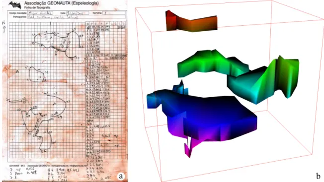
Fig. 1. Topographic information for the studied cave chamber. a) Copy of the notebook sketch based on in situ measurements; b) Digital 3D sketch based on in situ measurement data processed using Therion software (the studied chamber is the lower one) (Zabel, 2012).

west of Loulé city (Algarve). This cave extends about 80 m, has an entrance measuring 14 m, and a depth of about 20 m. It consists of two main chambers connected by a vertical narrow gallery of about 5 m (Fig. 1) (Zabel, 2012). Each chamber was surveyed independently because of the narrow vertical gallery, which does not allow a visual connection to be established between them. However, the work pre- sented in this paper deals only with the main chamber, the deeper and more complex one. The main chamber contains many geomorphological structures, including stalagmites, stalactites, flowstones, and columns (Fig. 2), favouring the quantitative approach taken in this paper.

DIGITAL SURVEY OF THE CAVE

The purpose of the cave survey was to measure and document the main chamber as well as to create an accurate map of its surface features. Accurate cave surveys provide the basic information to support investigations of cave geomorphology and evolution (Jaillet et al., 2011b). There are several techniques used for cave surveying, including the standard survey technique consisting of azimuth and distance measurements (e.g., Fig. 1), and relatively new techniques, such as photographic and scanning tools. Photogrammetric and laser-scanning techniques markedly improve the efficiency and accuracy of surveys, and allow realistic 3D models to be generated that can better characterize the interiors of caves and their features (Grussenmeyer & Guillemin, 2011; Remondino, 2011).

However, despite the possibility of making 3D reconstructions with photogrammetry, this method is difficult to implement in karst environments due to constraints such as darkness and dampness inside a cave, or even the degree of complexity of surface irregularities. Digital photogrammetry has been successfully used in recording cave paintings rather than documenting entire caves (Tsakiri et al., 2007).

In contrast, laser scanning, and more specifically Terrestrial Laser Scanning (TLS), is a good alternative to traditional surveying approaches because the technique can measure the position and dimensions of objects in 3D space and can be manipulated in dark environments. When applied to cave surveying, laser scanning quickly acquires the shapes of cavities as point clouds (see Point cloud data set for definition) with high precision, even if the process of data acquisition in the interior of a cave is a complex task due to the generally difficult access and the irregular and constrained working environment (see Fig. 2a).

Terrestrial laser scanning

Terrestrial laser scanning is a relatively new technology that can be used to conduct high-resolution surveys. TLS may employ three operating measurement principles: time-of-flight, phase-shift and triangulation-based (Beraldin et al., 2011). Terrestrial laser scanners provide detailed and highly accurate 3D data rapidly and efficiently facilitates the rapid acquisition of a huge number of 3D point measurements. One of the great advantages of this surveying method is the high-resolution surface geometry (down to 1 mm) that permits accurate and detailed surface reconstruction

and modelling to be performed as well as superior visualization to that of existing measurement technologies (Roncat et al., 2011).

The main chamber of the Algar do Penico Cave was surveyed with a TLS, specifically with a Leica ScanStation C10 time-of-flight laser scanner system mounted on a tripod. The specifications of this unit include a 360° horizontal field of view and a 270° vertical field of view and a modelled surface precision of 2 mm. The scanner emits pulses of green laser light that sweep across the chambers surface and send back spot measurements that provide x, y, and

z coordinates in a reference coordinate system given

by the scanner, each having an associated intensity value. The output data set resulted from the survey is called point cloud and represent an underlying sampled surface. When the photography acquisition mode is used in addition to the laser beam, colour variables are also captured.

Point cloud data set

First of all, a point cloud is a set of data points in a three dimensional coordinate system that represents the external surface of an object. Accordingly, the laser scanner captures a point cloud corresponding to the true positions of points where the laser pulse hits the studied object. The point cloud represents the shape and position of scanned surfaces relative to the position of the scanner, referred to here as the station. The shape of the chamber has many irregularities and thus it requires different scanner positions to avoid gaps as far as possible. In the present study, the chamber was scanned from three different stations.

The 3D laser scanner point cloud data were collected with a point spacing of 1 cm at a distance of 10 m from the laser-scanning device. This option allowed three point cloud data sets with about 15 × 106 _{points each} to be obtained. The coordinates of points scanned from different stations were in different local coordinate systems. Therefore, a registration process was applied to align individual point clouds into a single Cartesian reference datum. This was achieved through the use of artificial targets scanned during the survey (see Fig. 2b) (Tsakiri et al., 2007).

Table 1. Statistics for the surveyed targets inside the main chamber, where St is station number, Tg is target number, īis the mean intensity of the target, σi is the root mean square error of intensity, and # points is the number of scanned points for each target.

St Tg ī σi # points 01 01 1898 17 7835 02 1880 17 8343 03 1912 21 7067 04 1932 19 8692 05 1902 20 8301 06 1913 24 8860 02 01 1917 18 9539 02 1875 16 7222 05 1896 19 7652 06 1914 22 8945 03 01 1860 14 2549 03 1852 11 1468 04 1933 20 9591 05 1870 16 5052

Fig. 2. a) Photographs of the Algar do Penico main cave chamber, showing the complexity and irregularity of the landscape (view towards the west); b) Photography of a target.

Six registration targets were placed inside the chamber to establish at least three tie points to register the different local scanner locations into a single point cloud representing the whole chamber (Table 1). It should be noted that only four targets were common between stations St01 and St02 (Tg01, Tg02, Tg05, and Tg06) and between stations St01 and St03 (Tg01, Tg03, Tg04, and Tg05).

The registration process involved transformations of the original coordinates using mathematical affine transformations in 3D space. This process was performed using a Python; http://www.python.org/; routine and resulted in a root mean square error (RMSE) of about 3 mm for both pairs of scans.

The registration targets used here were 15.2 cm in diameter and flat with two concentric circles, and were designed to be easily identified (Barbarella & Fiani, 2012). Points obtained from targets present a well-differentiated intensity (i) relative to the chamber surface; a bimodal distribution of i values arises due to the existence of two distinct classes, one with a modal i value of −1298 (for the cave) and another

values of a reduce the number of laser beam points because of an increase in the lighted area.

However, the average intensity values do not appear to be affected by the angle between laser beam and target plane except when α is greater than about 45°. Accordingly, despite intensity values having been reported to be affected by surface material as well as distance and incidence angle (Voegtle et al., 2008; Kaasalainen et al., 2011), future research is still needed to evaluate the importance of the acquisition angle in order to better understand the intensity parameter and its relationship to the scanned material (Roncat et al., 2011; Krooks et al., 2013).

CAVE CHAMBER 3D MODEL

The laser scanning produced a point cloud of about 45 million points. Point clouds can be directly rendered or inspected and there are a significant number of practical application including, tomography, contouring, data visualization or even data comparing. In general, point clouds themselves are not directly usable in most 3D applications, and therefore they are commonly converted into 3D-mesh surfaces. In the present case study, point clouds do not provide enough information for identifying geomorphological structures, thus a surface model was needed and generated. In the next subsection we present the 3D-mesh generation process.

3D-mesh generation from point cloud

The computational representation of surfaces is a widely studied problem (e.g., see the list of examples in Roncat et al., 2011). Surfaces are usually represented by a collection of vertices, edges, and faces, known as a

polygonal mesh or polygonal soup, defining the shape

of a polyhedral object. The faces of the mesh usually consist of triangles or quadrilaterals, where each face corresponds to a set of three vertices or four vertices, respectively (Tobler & Maierhofer, 2006). A triangular 3D-mesh could be compared locally to Triangular

Irregular Network (TIN) in some surface interpolation.

Several commercial or open-source platforms can create surface models from point clouds. However, with a modal i value of +1925 (for the targets). Table 1

presents the average target intensity for points inside the blue disk sector (radius 5.1-15.2 cm, Fig. 2b) with values varying between 1850 and 1933 and with an RMSE σi of less than 21.

Targets Tg01 and Tg03 surveyed from station St03 present lower intensity values than do stations St01 and St02, as well as a lower number of collected points (# points) (Table 1). To explain these differences, we inspected the scans of the targets more closely.

Since targets are planar devices, all their scanned points lie on a single plane and the collected coordinates should satisfy the equation Ax + By + Cz = 1.

The system of equations for all points of each target can be expressed as a matrix equation:

Kw = 1 + ε (1)

where Km × 3 is the matrix of x, y, z coordinates for m target points, w is the vector of plane coefficients, 1 is the m-dimension all-ones vector, and ε is the m-dimension residuals vector:

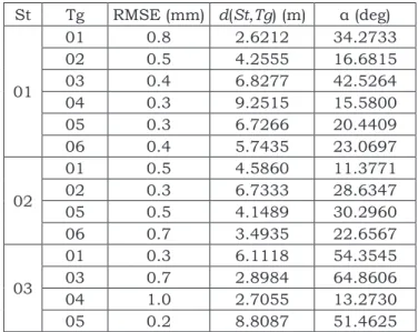
Table 2. Measurements of target precision expressed as root mean square error (RMSE). d(St, Tg) is the distance between stations and targets, and α is the angle between the laser beam and the target plane.

St Tg RMSE (mm) d(St,Tg) (m) α (deg) 01 01 0.8 2.6212 34.2733 02 0.5 4.2555 16.6815 03 0.4 6.8277 42.5264 04 0.3 9.2515 15.5800 05 0.3 6.7266 20.4409 06 0.4 5.7435 23.0697 02 01 0.5 4.5860 11.3771 02 0.3 6.7333 28.6347 05 0.5 4.1489 30.2960 06 0.7 3.4935 22.6567 03 01 0.3 6.1118 54.3545 03 0.7 2.8984 64.8606 04 1.0 2.7055 13.2730 05 0.2 8.8087 51.4625 u = [1 1 … 1]T _{and ε = [ε} 1 ε2 … εm]T

Equation (1) can be solved using least-square adjustments to estimate w,

w = (KT _K)−1 _KT ₁

The residuals values εi correspond to the distance between each point datum and the average plane. They can thus be estimated from Equation (1). The RMSE of residuals calculated using:

RMSE =

was computed and the results are presented in Table 2. Globally, RMSE is ≤ 1 mm, revealing the very high precision of coordinates even for targets Tg01 and Tg03 of station St03.

Let now n be a vector perpendicular to the plane

of a target, and consider T the centre of this target, and S the centre of the station, which does not lie on the target plane. In this case, vectors n and ST

are collinear when the laser beam hits the centre of the target perpendicularly to the target plane. Accordingly, the computed angle a between vector

n and ST represents the angle of the target plane in

relation to the laser beam and is equal to 0 when ST

is orthogonal to the target plane (Table 2).

Targets Tg01 and Tg03 from station St03 show high values of α (≈ 54° and 65°, respectively; Table 2), which explains the low number of points collected for these targets from station 3. As expected, these high

in the present work, we used MeshLab software; http://meshlab.sourceforge.net (Cignoni et al., 2008), which is a free, open-source software for mesh processing and editing and which generates a triangular 3D-mesh. This software works with the most common 3D file formats, such as PLY, STL, OBJ, 3DS, COLLADA, PTX, PTS, XYZ, ASC, X3D, and VRML. Several algorithms

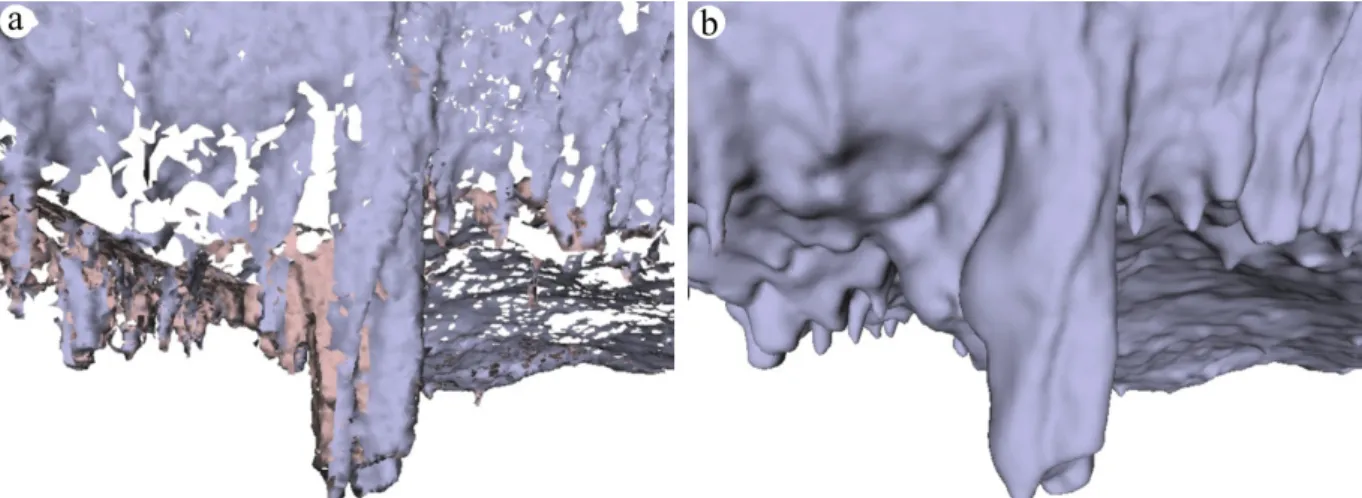
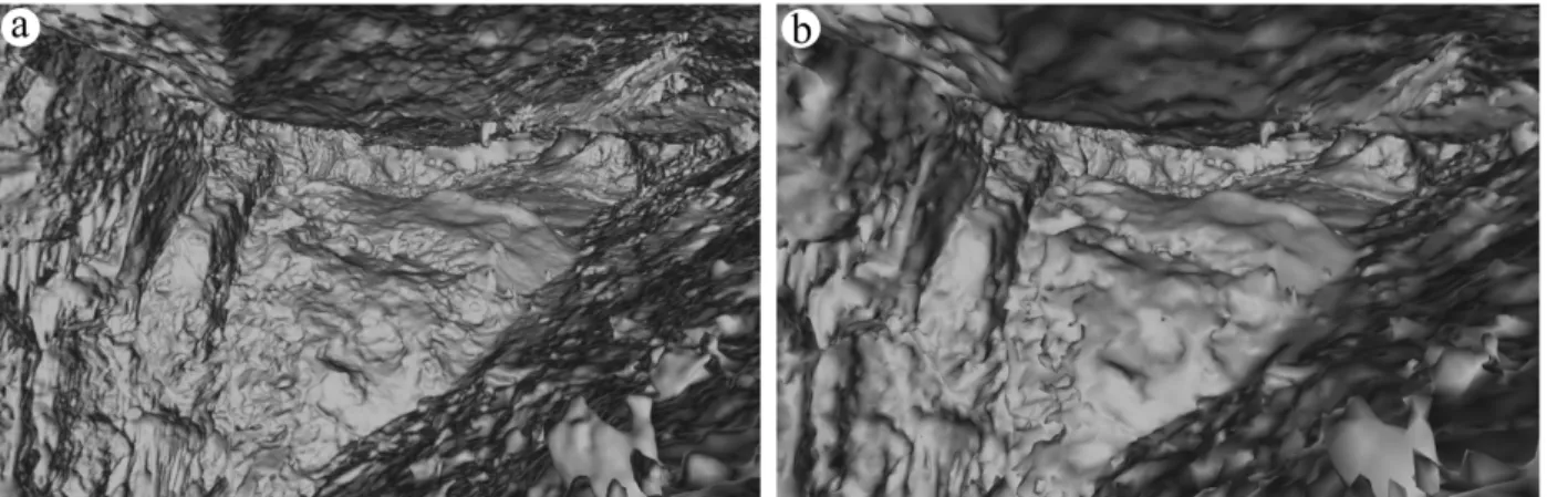
Fig. 3. Example extracted from cave 3D meshes generated with (a) the Ball - Pivoting Algorithm and (b) Poisson Surface Reconstruction.

Table 3. Examples of parameter variation (number of faces and PLY file size in MB) in 3D meshes generated from a point cloud containing several interesting stalactites (233940 point cloud input data) and from the whole cave survey (44399724 point cloud input data) for octree depth values ranging between 10 and 14 and samples per node (spn) of 1 and 10-3_.

available in MeshLab can be used to reconstruct surfaces from point clouds. We explored two of them for possible use in this study, namely, the Ball-Pivotting

Algorithm (BPA) and Poisson Surface Reconstruction

(PSR) (see Fig. 3).

The BPA computes a triangular mesh to interpolate a given point cloud using a ball of fixed radius that

traverses the point cloud by pivoting front edges and attaching triangles to the mesh (Bernardini et al., 1999). In the present case, this algorithm resulted in a mesh with a large number of face gaps (Fig. 3a). This problem may occur in laser scan surveys due to problems with visibility and/or complexity (Chalmovianský & Jüttler, 2003). One way to reduce the number of these holes would have been to increase the number of stations of the laser scan during the survey. However, due to the physical characteristics of the cave chamber, such a solution would have been very difficult to implement.

Unlike the BPA, PSR requires oriented vertex normals as input data. These normals can be computed as equivalent to a normalized average of the surface normals to the faces containing that vertex (Glassner, 1994). The vertex normals allow the orientations of the faces to be determined.

PSR is based on the observation that the normal field of the boundary of a solid can be interpreted as the gradient of the solid’s indicator function. Therefore, given a set of oriented points sampling the boundary of a solid, a 3D-mesh can be obtained by transforming the

oriented point samples into a continuous vector field in 3D. This is performed by finding a scalar function whose gradients best match the vector field and then extracting the appropriate isosurface (Kazhdan et al., 2006). Although a thorough analysis of this algorithm is beyond the scope of this paper, it is worth noting that the vertices of the faces of these meshes do not coincide with the points of the survey.

As shown in Fig. 3, PSR (Fig. 3b) copes much better with missing data than does the BPA (Fig. 3a), and therefore we used PSR for the cave chamber model reconstruction (presented below).

3D-mesh selection

To create a 3D-mesh that best represented the input point cloud of the cave chamber, we tested different input parameters used for the PSR method. Two examples of point clouds were used (Table 3), namely, the whole cave survey, with approximately 45 million points (referenced as Full cave in Table 3), and a sample of it containing some interesting stalactites, with around 230 thousand points (referenced as Stalactites in Table 3).

# faces file size (mb)

3D-mesh Stalactites Full cave Stalactites Full cave

10 depth, 1 spn 541816 2623790 26.5 132.4 10 depth, 10-3 spn 846928 2658050 41.8 134.2 11 depth, 1 spn 550168 10038522 26.9 525.4 11 depth, 10-3 spn 869730 10549762 43.0 552.5 12 depth, 1 spn 555128 31531448 27.1 1700.0 12 depth, 10-3 spn 875334 36680494 43.2 1988.1 13 depth, 1 spn 573190 58042828 28.9 3190.8 13 depth, 10-3 spn 893608 * 44.2 * 14 depth, 1 spn 637718 * 31.3 * 14 depth, 10-3 spn 960294 * 47.5 *

The surface obtained with PSR has a variable level of detail depending on the input parameters octree depth and samples per node. Accordingly, we generated 3D meshes with octree depth values varying from 10 to 14 and samples per node varying from 1 to 10-3 _{(Table 3).} Samples per node is usually presented in the literature as the minimum number of sample points that should

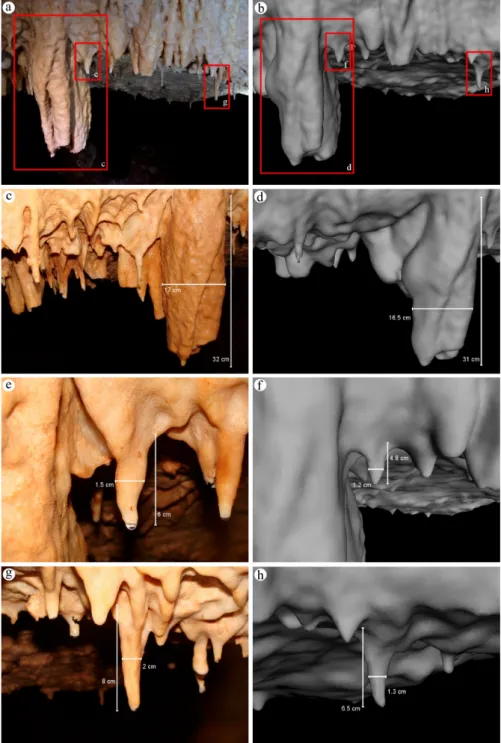
Fig. 4. Comparisons of feature measurements between photographs of actual structures (left-hand images: a, c, e, g) and the generated 3D-mesh with an octree depth of 14 and 10-3 samples per node (right-hand images: b, d, f, h). Note the measurements of the structures made either directly in the cave or in the 3D model.

fall within an octree node as the octree construction is adapted to sampling density. For noise-free data, a value between 1.0 and 5.0 should be used and for noisy data between 15.0 and 20.0. However, this parameter is implemented in MeshLab as a floating variable, suggesting that other values than integers may be considered. In our study, due to the irregularity of the surfaces, we explored extreme values, and for this reason we used values from 1 to 10-3_.

The octree depth parameter is the maximum depth of the tree that is used for the surface reconstruction. An increase in the depth increases the detail of the surface. For octree depths ranging between 10 and 12, the number of faces increases by only 3% for the stalactite data set, whereas for the full point cloud it increases by 92%. It should be noted that it was not possible to generate a 3D-mesh with an octree depth of 14 for the full point cloud acquired from the TLS survey due to computational capacity. We used an Intel Core i7 processor running at 3.40 GHz with 8 GB of RAM and a NVIDIA Quadro 4000 graphics card (with 2 GB of dedicated memory), running the MeshLab software under the 64-bit Ubuntu 12.04 LTS version, a Linux-based computer operating system.

The samples per node parameter is related to the sample points that should fall within an octree node, because the octree construction is adapted to sampling density (Kazhdan et al., 2006). This value is provided by the user and depends on the noise of the samples. When the value of samples per node is decreased, the surface is represented with more detail, increasing the number of faces and the size of the file stored in PLY format (Table 3).

more than 50% of the smaller structures appear in the 3D model. We also measured the size of several structures and concluded that the mesh generated with an octree depth of 14 and 10-3 _{samples per node} was the 3D model that better represented the physical characteristics of small structures such as those shown in Fig. 4.

For the identification of small geomorphological structures, such as those presented in Fig. 4, the 3D-mesh is generated only for a specific area, thus allowing the processing of a model with an octree depth of 14 and 10-3 _{samples per node. We verified} that for the mesh generated with an octree depth of 14 and 1 sample per node, only 30% of the structures appear in the 3D model. For the mesh generated with an octree depth of 14 and 10-3 _{samples per node,}

3D data visualization on the Web

As a consequence of advances in both computer hardware and internet connection speeds, Web 3D sites that include 3D models where users navigate and interact through a 3D graphical interface are being increasingly employed in different do- mains. The possibility of making 3D data available on the Web is of particular interest in the geospatial field. Such availability provides researchers with the opportunity

to visualize, navigate, and interact with 3D data on a simple Web browser. Therefore, we aimed to map and visualize online geomorphological structures of the cave interior in an interactive way. It is now possible to integrate 3D content on the Web directly into the browser without plug-ins or additional components. This is the approach presented in this paper in which X3D, WebGL, and X3DOM were used to enable 3D visualization and navigation of the interior of the Algar do Penico cave in several different Web browsers. X3D is used to represent the cave chamber 3D model and is inserted on the user side for visualization in WebGL-supported browsers with the X3D document object model (X3DOM) technique. This is possible because: (i) X3D is the ISO standard XML-based file format for representing 3D computer graphics (Behr et al., 2009); (ii) WebGL is an open standard software library for a low-level 3D graphics API based on OpenGL that generates interactive 2D and 3D graphics on any browser without installing additional plug-ins (Behr et al., 2009; Prieto et al., 2012); and (iii) X3DOM is

Fig. 5. Example of the cave chamber 3D-mesh obtained using Poisson Surface Reconstruction with an octree depth of 11 and 1 sample per node (a) and its simplification after the decimation process (b). Note the similarity of the 3D-mesh representations to the picture in Fig. 2a.

Table 4. Tests of download speed between three mesh sizes generated after different decimations based on the original model with an octree depth of 11 and 1 sample per node, which had 10038522 faces.

an open-source framework that integrates HTML5 and X3D on top of WebGL (Behr et al., 2009). Thus, X3DOM manipulates X3D scenes as HTML5-DOM elements, rendered via WebGL with no plug-in required, to display the X3D content.

However, the 3D-mesh size is a problem for the efficiency and interactivity of visualization in real time on the Web. As mentioned above, the 3D-mesh generated with the PSR method with an octree depth of 11 and 1 sample per node for the entire cave chamber has about 10 million faces (Table 3 and Fig. 5a). A compromise has to be achieved between the complexity of the 3D-mesh, the realistic visualization of the chamber, and real-time interaction (Fig. 5). Accordingly, to produce a lighter model for visualization on a Web browser, we decided to simplify the cave chamber 3D-mesh by applying geometry removal operations. These operations are referred to as mesh decimation and consist of the iterative removal of geometrical units such as vertices, edges, and triangle faces (Heckbert & Garland, 1999; Gotsman et al., 2002).

For the 3D-mesh simplification, we used the MeshLab multi-edge decimation function called Quadratic Edge

Collapse Decimation. This function removed the

multi-edge mesh together with the associated triangles, and then connected the adjacent vertices to the new vertex (Chen et al., 2007).

Three simplifications were generated from the 3D-mesh with an octree depth of 11. Table 4 presents the number of triangular faces and the size of each simplified 3D-mesh file in X3D format. Tests of download time were performed in a localhost environment. Waiting times varying between 7 and 60 s were measured.

decimation (%) # faces file size (mb) download _{time (s)}

90 998856 60.2 60

95 499486 29.8 19

97 249934 14.6 7

Considering the download times presented in Table 4, we selected the 3D-mesh with 249934 faces for the Web 3D visualization (see Fig. 5b). This 3D-mesh takes

about 7 s to be ready for real-time interaction in a Web browser and looks very similar to the original model and also to the real environment (see Figs. 2a and 5).

IDENTIFICATION AND RECOGNITION OF STRUCTURES FROM THE 3D-MESH As illustrated in the Algar do Penico Cave example (Fig. 4), laser scan surveys can deal with both meso- and micromorphological features. These small features represent structures, namely stalactites and stalagmites, that are important in the study of karst hydrogeology and geomorphology (Hajri et al., 2009).

Here, we present two algorithms that allow stalactite extremities to be localized and contour lines to be sketched with a predefined equidistant between contours for a 3D model. These tools are more than just visual, as they allow users to collect additional analytical information. Both algorithms run in linear time with respect to the number of vertices and edges. They were tested with the most complex model for the specific area, which has 58042828 triangles (see Table 3).

However, triangular meshes usually consist of a collection of triangles without any associated explicit topological information. For 3D-mesh analysis, we adopted a graph

structure to disclose topological adjacency relationships between triangle vertices. Graphs are often drawn as node-link diagrams in which the nodes are represented as vertices and links as binary relations between vertices (see Silvestre et al., 2013 for more details). Several data structures are available to store graphs. We adopted the adjacency list data structure, in which there is a list of adjacent vertices for each vertex. For computational purposes, adjacency information was organized with the help of Python dictionaries, which correspond to associative arrays or hash tables in other programming languages (Beazley, 2006).

Local minima

Stalactite extremities correspond to local minima in the 3D-mesh. A local minimum in the 3D-mesh surface is a vertex v of the mesh such that its z-coordinate is smaller than the z-coordinates of all adjacent vertices of v. This local minimum is a stalactite extremity when its normal vector n = (0, 0, nz) and nz < 0.

For the graph G = (V, E), de ined from a 3D-mesh, Algorithm 1 returns a list of vertices such that its

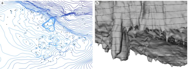
Fig. 6. Plane view with local minima representing the lower tips of stalactites and contour lines (a), and a 3D view of the same area (b). The 3D-mesh used in the diagrams was generated with an octree depth of 14 and 10−3 _{samples per node.}

Algorithm 1. Local minima algorithm.

z-coordinates are less than or equal to the z-coordinates

of all adjacent vertices and the vector normal to the surface is downward oriented.

The local minima returned by Algorithm 1 for a partial view of the 3D-mesh with an octree depth of 14 and 10−3 _{samples per node (see Table 3) can be} presented in a map or plane view or directly on the 3D-mesh (Figs. 6a and 6b, respectively). In the latter, it is possible to verify that local minima are indeed coincident with stalactite extremities.

With slight modifications, Algorithm 1 returns local maxima vertices corresponding to stalagmite extremities.

Contour lines

Contour lines (or contours) on nonflat surfaces are lines connecting points of the same elevation. For a 3D-mesh, if the z0 elevation contour line intersects an edge of the model, then the contour line has two segments that lie on the triangles T1 and T2 incident on that edge.

Assuming the graph G = (V, E) and the elevation z0 as input, Algorithm 2 returns the collection of the segments of the polyline Cz0 that represent the contour of elevation z0.

The algorithm was used to compute a collection of contours with a predefined equidistant interval between consecutive lines.

Contours provide rich information on cave chamber morphology. They help identify smooth, flattened, or steep surfaces as well as the positioning of specific alignments. Fig. 7b shows the ceiling surface of the cave model from a top-view perspective with superimposed 15 cm equidistant contour lines, where cave relief and preferred alignments are highlighted and thus easily recognized.

Algorithm 2. Contour lines algorithm. DISCUSSION

TLS is an emerging technology that has been applied in various situations including the monitoring of tunnels during the construction phase, the documentation of cultural heritage, and the inspection of industrial and technical facilities. To date, there have been several case studies reporting the application of TLS to cave mapping and rock art documentation (González-Aguilera et al., 2009; Beraldin et al., 2011; Jaillet et al., 2011a; Roncat et al., 2011; Sadier et al., 2011).

Fig. 7. Ceiling surface of the cave chamber 3D-mesh from a top-view perspective (a), and the same 3D-mesh with 15 cm equidistant contour lines (b). This 3D-mesh was generated with an octree depth of 11 and 1 sample per node.

In addition to cave mapping, the present paper has focused on 3D-mesh analysis, including the determination of local minima and contour lines from 3D-mesh (Identification and recognition of structures

from the 3D-mesh) and on Web publishing for

interactive visualization (3D data visualization on the

Web) The entire project has been developed using only

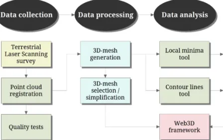
a small number of computing solutions (i.e., Python, MeshLab, X3D, WebGL, and X3DOM) for carrying out all the tasks from the TLS cave survey to the generation and analysis of the 3D-mesh (see Fig. 8 for details of the work flow). Besides their effectiveness, these computing options bear no financial cost.

There are several commercially software that offer out of the box and robust solutions for 3D-mesh generation, visualization, interpretation and analysis, such as

Leica Cyclone, 3DReshaper or Geomagic Wrap (Pucci

& Marambio, 2009; Roncat et al., 2011). Nevertheless, there are open-source solutions also robust and easy to use, such as MeshLab and CloudCompare. In this study, we chose MeshLab, which is an open-source software able to deal with closed 3D environments, and Python programming language. The framework for 3D Web visualization is also based on open-source components, namely using X3D as the 3D data format and WebGL and

Fig. 8. Work flow showing all tasks from data collection to processing and analysis. Python programming language (green boxes) was used for the registration, quality tests, identification of local minima, and determination of contour lines. MeshLab software (blue boxes) was used to process data, namely for 3D-mesh generation and selection/ simplification. The 3D-mesh and its local minima and contour lines were made available with the development of a Web3D framework.

X3DOM to generate interactive 3D scenes. Accordingly, there is no need to install new software or additional plug-ins to visualize and interact with the 3D model in a Web browser. Furthermore, the possibility of visualizing 3D meshes with both contour lines and speleothem extremities (Fig. 6b) brings new application perspectives to the study of karst.

Large 3D-mesh file sizes could pose problems for visualization and interactivity on the Web. To solve this problem, Lavoué et al. (2013) proposed a method that consists of progressive 3D-content compression on the Web. In our case, we adopted a different solution whereby a 3D-mesh was simplified using a decimation process that seems quite efficient in maintaining the first-order size of the chamber and even the smaller structures (Figs. 5 and 6). This is supported by the results obtained when evaluating the differences between triangular meshes with the Metro tool, which allows pairs of surfaces (e.g., a triangulated mesh and its simplified representation) to be compared by adopting a surface-sampling approach (Cignoni et al., 1998). The results show that the Hausdorf distance (i.e., the largest distance) between the stalactite model (563405 faces) and its simplified model at 97% (with about 16902 faces) is 12 mm. The same test was

made for a partial cave chamber model with 7449484 faces and its simplification at 97% (223216 faces), which yielded a value of 25 mm. This test was made for a partial cave chamber model instead of the full model due to constraints of the Metro tool. The values obtained for the Hausdorf distance are both less than 0.2% of the bounding-box diagonal.

The other problem arising from the size of the point cloud data set lies in generating a 3D-mesh for the entire cave with a high octree depth parameter, as is evident in Table 3. Nevertheless, when selecting a specific region exhibiting several stalactite-type structures, the generation of a 3D-mesh with an octree depth of 14 was successful, as shown in Fig. 4. The high level of detail obtained in such a model is noticeable by the presence of small structures measuring about 1 cm. Furthermore, it is important to note that the compared dimensions of the structures obtained in the model and the actual structures in the cave

differ by only 1 cm for the major features and by about 2 cm for the smaller ones. These smaller-scale features, which are typically not represented on standard cave maps, can thus now be well defined. The combination of TLS survey and 3D-mesh generation delivering high-resolution or very high high-resolution 3D models enables meso- and micromorphological features to be mapped, thereby providing a significant improvement in the level of detail available for studies of cave morphology compared with previous approaches.

CONCLUSIONS AND FUTURE WORK This study has shown that surveying a cave using Terrestrial Laser Scanning (TLS) allows high-resolution point cloud data sets to be obtained that accurately and precisely represent the surface geometry of the studied cave. Unlike other close-range methods for cave surveying, TLS is able to be used for surveys in environments with difficult access and a lack of light. However, some problems exist regarding the massive data collection and the work environment inside the cave with respect to shadow areas and point cloud gaps. These difficulties were successfully over- came using free and open-source applications generating 3D meshes with different levels of detail, with the highest levels being used for 3D-mesh analysis and the lowest levels for 3D data on the Web, but still preserving the surface bounding and the most important geomorphological structures. The results obtained in the present work are linked to the point cloud survey resolution, i.e., 1 cm at 10 m from the laser scan. In the subsequent data-processing phase, the parameter settings for the surface reconstitution process allow developing models that have different levels of accuracy and precision. We do believe that the same type of results can be obtained in other caves as long as the parameter adjustments are adequate to the dimension and morphology of the cave.

Besides visualization platforms, researchers also need tools to map, measure, and analyse geomorphological changes through time. In this context, the development of tools for the automatic identification and characterization of speleothems and of other physical structures inside caves is one of the contributions of the present study. We built a high-precision model of a cave chamber, implemented algorithms that allowed the identification of speleothem extremities (namely, stalactites and stalagmites) and contour lines, and made the model available on a 3D Web interactive platform with no need for plug-ins. The availability of the Algar do Penico Cave 3D model in a Web3D environment is an interesting development in the geospatial field, where both researchers and the general public can navigate and interact with the cave chamber. The next steps in this continuing line of research will focus on identifying the full range of structures comprising the cave surface and on how stalactites and/or stalagmites form watersheds.

ACKNOWLEDGEMENTS

This work was supported by the Portuguese government and EU – funding, through the FCT – Fundação para a Ciência e Tecnologia funding of the SIPCLIP project

PTDC/AAC-CLI/100916/2008 and partially of the project PEst-OE/MAR/UI0350/2011 (CIMA). We are grateful to the Centre for Marine and Environmental Research (CIMA) and Geonauta’s speleological association for their support. We also thank the editor and the reviewers for their support and comments, which helped us to improve the manuscript.

REFERENCES

Barbarella M. & Fiani M., 2012 – Landslide monitoring using

Terrestrial Laser Scanner: georeferencing and canopy filtering issues in a case study. ISPRS – International

Archives of the Photogrammetry, Remote Sensing and Spatial Information Sciences, XXXIX-B5: 157-162.

http://dx.doi.org/10.5194/isprsarchives-XXXIX-B5-157-2012

Beazley D., 2009 – Python Essential Reference, 4th edition. Addison-Wesley Professional: 744 p.

Behr J., Eschler P., Jung Y. & Zöllner M., 2009 – X3DOM:

a DOM-based HTML5/X3D integration model. In: Spencer

S.N. (Ed.) – Proceedings of the 14th _{International Conference}

on 3D Web Technology (Web3D ‘09). New York, NY, USA:

ACM: 127-135.

http://dx.doi.org/10.1145/1559764.1559784

Beraldin J.-A., Blais F. & Lohr U., 2010 – Laser scanning

technology. In: Vosselman G. & Maas H. (Eds) – Airborne and terrestrial laser scanning. Whittles Publishing: 1-42.

Beraldin J.-A., Picard M., Bandiera A., Valzano V. & Negro F., 2011 – Best practices for the 3D documentation of the Grotta

dei Cervi of Porto Badisco, Italy. In: Beraldin J.A., Cheok

G.S., McCarthy M.B., Neuschaefer-Rube U., Baskurt A.M., McDowall I.E. & Dolinsky M. (Eds) – Three-dimensional

imaging, interaction, and measurement. Proceedings of

SPIE-IS&T Electronic Imaging, SPIE Vol. 7864: 15. http://dx.doi.org/10.1117/12.871211

Bernardini F., Mittleman J., Rushmeier H., Silva C. & Taubin G., 1999 – The Ball-Pivoting Algorithm for surface

reconstruction. IEEE Transactions on Visualization and

Computer Graphics 5 (4): 349-359. http://dx.doi.org/10.1109/2945.817351

Budaj M. & Stacho M., 2008 – Therion – digital cave maps. In: Spelunca. Spelunca Mémoires (French Federation of Speleology) 33: 138-141.

Chalmovianský P. & Jüttler B., 2003 – Filling holes in

point clouds. In: Wilson M.J. & Martin R.R. (Eds.) – Mathematics of surfaces, Proceedings of the 10th _IMA

International Conference. Springer, 2768: 196-212. http://dx.doi.org/10.1007/978-3-540-39422-8_14

Chen H., Luo X. & Ling R., 2007 – Surface simplification

using multi-edge mesh colapse. In: Fourth International Conference on Image and Graphics, 2007. ICIG 2007:

954-959. http://dx.doi.org/10.1109/ICIG.2007.91

Cignoni P., Rocchini C. & Scopigno R., 1998 – Metro:

measuring error on simplified surfaces. Computer

Graphics Forum, 17 (2): 167-174.

http://dx.doi.org/10.1111/1467-8659.00236

Cignoni P., Callieri M., Corsini M., Dellepiane M., Ganovelli F. & Ranzuglia G., 2008 – Meshlab: an

open-source mesh processing tool. In: Scarano V., De Chiara

R. & Erra U. (Eds) – Eurographics Italian Chapter

Conference, 2008: 129-136.

http://dx.doi.org/10.2312/LocalChapterEvents/ ItalChap/ItalianChapConf2008/129-136

Fairchild I.J. & Baker A., 2012 – Speleothem Science: From Process to Past Environments. Wiley-Blackwell, Chichester: 432 p.

Lavoué G., Chevalier L. & Dupont F., 2013 – Streaming

compressed 3D data on the web using JavaScript and WebGL. In: Proceedings of the 18th _{International}

Conference on 3D Web Technology (Web3D ‘13). ACM,

New York, NY, USA: 19-27.

http://dx.doi.org/10.1145/2466533.2466539

Prieto I., Izkara J. & Delgado F., 2012 - From point cloud

to web 3D through CityGML. In: Proceedings of the 18th _{International Conference on Virtual Systems and}

Multimedia (VSMM), 2-5 Sept. 2012: 405-412.

http://dx.doi.org/10.1109/VSMM.2012.6365952

Pucci B. & Marambio A., 2009 – Olerdola’s Cave,

Catalonia: a virtual reality reconstruction from terrestrial laser scanner and GIS data. In: 3D virtual reconstruction and visualization of complex architectures, Proceedings

of ISPRS International Workshop 3D-ARCH 2009. Remondino F., 2011 – Heritage recording and 3D modeling

with photogrammetry and 3D scanning. Remote Sensing,

3 (6): 1104-1138.

http://dx.doi.org/10.3390/rs3061104

Roncat A., Dublyansky Y., Spötl C. & Dorninger P., 2011 –

Full-3D surveying of caves: a case study of Märchenhöhle (Austria). In: Marschallinger R. & Zobl F., 2011 – Mathematical geosciences at the crossroads of theory and practice, Proceedings of the IAMG2011 Conference,

September 5-9 2011, Salzburg, Austria: 1393-1403.

http://dx.doi.org/10.5242/iamg.2011.0074

Sadier, B., Lacave, C., Delannoy, J.-J. & Jaillet, S., 2011 – Relevés lasergrammétriques et calibration sur calcite

de morphologies externes de spéléothèmes pour une étude paléo-sismologique du Liban. In: Jaillet S., Ployon

E. & Villemin T. (Eds), 2011 – Images et modèles 3D

en milieux naturels. Collection EDYTEM, 12: 137-144. Silvestre I., Rodrigues J.I., Figueiredo M. & Veiga-Pires

C., 2013 – Framework for 3D data modeling and web

visualization of underground caves using open source tools. In: Proceedings of the 18th _{International Conference}

on 3D Web Technology (Web3D ‘13). ACM, New York,

NY, USA: 121-128.

http://dx.doi.org/10.1145/2466533.2466549

Tobler R. & Maierhofer S., 2006 – A mesh data structure

for rendering and subdivision. In: Jorge J. & Skala V.

(Eds.), 2006 - The 14th International Conference in

Central Europe on Computer Graphics, Visualization and Computer Vision (WSCG’2006) Short Communication

Papers Proceedings: 157-162.

Tsakiri M., Sigizis K., Billiris H. & Dogouris S., 2007 – 3D laser

scanning for the documentation of cave environments. In: Underground space: expanding the frontiers, Proceedings of the 11th _{ACUUS Conference, September 10-13 2007,} Athens, Greece: 403-408.

Voegtle T., Schwab I. & Landes T., 2008 – Influences of

different materials on the measurements of a terrestrial laser scanner (TLS). In: ISPRS – International Archives

of the Photogrammetry, Remote Sensing and Spatial Information Sciences, XXXVII-B5: 1061-1066.

Zabel F., 2012 – Topografia da Cavidade – Algar do Penico. Relatório do Levantamento e Esboço: 11 p.

Ford D.C. & Williams P., 2007 – Karst Hydrogeology and Geomorphology. Wiley: 576 p.

http://dx.doi.org/10.1002/9781118684986

Glassner A., 1994 – Building vertex normals from an

unstructured polygon list. In: Heckbert P.S. (Ed.)

– Graphics gems IV. Academic Press Professional, Inc., San Diego, CA, USA: 60-73. http://dx.doi. org/10.1016/B978-0-12-336156-1.50015-X

González-Aguilera D., Muñoz-Nieto A., Gómez-Lahoz J., Herrero-Pascual J. & Gutierrez-Alonso G., 2009 – 3D digital

surveying and modelling of cave geometry: application to Paleolithic rock art. Sensors, 9 (2): 1108-1127.

http://dx.doi.org/10.3390/s90201108

Gotsman C., Gumhold S. & Kobbelt L., 2002 – Simplification

and Compression of 3D Meshes. In: Iske A., Quak E. &

Floater M.S. (Eds) – Tutorials on multiresolution in geometric

modelling. Mathematics and visualization, 2002. Berlin

Heidelberg: Springer: 319-361.

http://dx.doi.org/10.1007/978-3-662-04388-2_12

Grussenmeyer P. & Guillemin S., 2011 – Photogrammetry

and laser scanning in cultural heritage documentation: an overview of projects from INSA Strasbourg. In: Mohamed

M. & Grussenmeyer P. (Eds.) – Geomatics in the City,

Proceedings of the GTC2011 Symposium, Jeddah, Saudia Arabia, May 10-13 2011: 8 p.

http://geomaticsksa.com/GTC2011/S4/PDF/21.pdf

Hajri S., Sadier B., Jaillet S., Ployon E., Boche E., Chakroun A., Saulnier G.-M. & Delannoy J.-J., 2009 – Analyse

spatiale et morphologique d’une forêt de stalagmites par modélisation 3D dans le réseau d’Orgnac. Karstologia,

53: 1-14.

http://hal-sde.archives-ouvertes.fr/halsde-00457291

Heckbert P. S. & Garland M., 1999 – Optimal triangulation

and quadric-based surface simplification. Journal of

Computational Geometry: Theory and Applications, 14 (1-3): 49-65.

http://dx.doi.org/10.1016/S0925-7721(99)00030-9

Jaillet S., Ployon E. & Villemin T. (Eds), 2011a – Images et

modèles 3D en milieux naturels. Collection EDYTEM: 216 p.

Jaillet S., Sadier B., Hajri S., Ployon E. & Delannoy J.-J., 2011b – Une analyse 3D de l’endokarst: applications

lasergrammétriques sur l’aven d’Orgnac (Ardèche, France).

Géomorphologie: relief, processus, environnement, 4: 379-394.

http://dx.doi.org/10.4000/geomorphologie.9594

Kaasalainen S., Jaakkola A., Kaasalainen M., Krooks A. & Kukko A., 2011 – Analysis of incidence angle and distance

effects on terrestrial laser scanner intensity: search for correction methods. Remote Sensing, 3 (10): 2207-2221. http://dx.doi.org/10.3390/rs3102207

Kazhdan M., Bolitho M. & Hoppe H., 2006 – Poisson

surface reconstruction. In: Proceedings of the fourth Eurographics symposium on Geometry Processing (SGP ‘06). Eurographics Association, Aire-la-Ville,

Switzerland, Switzerland: 61-70.

Krooks A., Kaasalainen S., Hakala T. & Nevalainen O., 2013 – Correction of intensity incidence angle effect in terrestrial

laser scanning. ISPRS Annals of the Photogrammetry,

Remote Sensing and Spatial Information Sciences, II-5/ W2: 145-150. http://dx.doi.org/10.5194/isprsannals-II-5-W2-145-2013