FROM CLASSICAL REGRESSION ANALYSIS
TO QUALITATIVE ANALYSIS:
A SHARE PRICE fsQCA EMPIRICAL APLICATION
Fábio André Pereira Luís
Dissertation submitted as partial requirement for the conferral of
Master in Finance
Supervisor:
Prof. José Dias Curto, Associate Professor, ISCTE-IUL Business School, Department of Quantitative Methods for Management and Economics
This thesis studies the difference between classical regression analysis and qualitative comparative analysis. Several authors argue that any preference for one approach over the other one should not be taken since both should complement themselves and therefore both should be used. This research is composed by a sample of 265 enterprises listed in European stock markets, using financial information of 2016, through the application of a classical regression analysis and a qualitative comparative analysis. More than testing the impact of the size of the company, the leverage level, the book value per share, the earnings per share, the return on asset, the cashflow from operations on asset and the ownership by a billionaire on the share price, this research aims at comparing classical regression analysis and comparative qualitative analysis through the results obtained from the empirical assessment. The main conclusion shows that qualitative comparative analysis helps to expand the comprehension regarding the conditions needed to achieve the outcome. In fact, the study contributes for the corroboration that regression analysis can be complemented by qualitative comparative analysis. The main limitations of this study are related to the use of a one-year data, which is also relatively outdated, since refers to 2016.
Keywords
Regression Analysis, Qualitative Comparative Analysis, Fuzzy-set, Share Price
JEL Classification System C02, C31
Resumo
Esta tese estuda a diferença entre a análise de regressão clássica e a análise comparativa qualitativa. Vários autores argumentam que qualquer preferência sobre uma delas não deve ser tida em consideração, uma vez que ambas se devem complementar e têm de ser utilizadas. Para esse propósito, foi utilizada uma amostra constituída por 265 empresas listadas em bolsas de mercado europeias, utilizando informação financeira de 2016, que será utilizada quer na análise de regressão, quer na análise comparativa qualitativa. Mais do que testar o impacto da dimensão da empresa, do nível de endividamento, do valor contabilístico das ações, dos ganhos por ação, do retorno dos ativos, dos fluxos de caixa das operações sobre os ativos e da estrutura patrimonial no preço das ações, este estudo pretende comparar as diferentes metodologias utilizadas através dos respetivos resultados. As principais conclusões do estudo revelam que a análise qualitativa comparativa ajuda a compreender as condições necessárias para alcançar o resultado desejado. De facto, esta investigação corrobora estudos anteriores que concluem que a análise de regressão pode ser complementada com a análise comparativa qualitativa. As principais limitações deste trabalho estão relacionadas com o uso de uma base de dados referente a um só ano que, adicionalmente, também está relativamente desatualizada visto que se refere a 2016.
Palavras chave
Análise de Regressão, Análise Comparativa Qualitativa, Conjuntos Incertos, Preço das Ações
Sistema de Classificação JEL C02, C31
Firstly, I would like to thank my supervisor, Prof. José Dias Curto, for the support given to elaborate and write this dissertation, especially because the respective scope includes a type of analysis that is not widely known. In addition, I also thank Prof. Isabel Lourenço, who supported all efforts regarding the data base.
Secondly, I would like to thank my parents for the support given during my second round of my higher education.
Last but not least, I would like to thank my wife for being by my side during these years, prompting me every day that the dissertation was to be done and never letting me give up.
I
Index
1. Introduction ... 1
2. Literature review ... 3
2.1. Classical regression analysis ... 3
2.1.1. General remarks ... 3
2.1.2. The goodness-of-fit of a model ... 5
2.1.3. Estimation ... 5
2.1.4. Inference ... 7
2.2. Limitations of classical regression analysis ... 8
2.3. Complexity Theory ... 11
2.4. Qualitative comparative analysis ... 13
2.4.1. fsQCA, a kind of QCA ... 14
2.4.2. Methodology of QCA ... 16
2.4.3. An empirical example ... 17
2.5. Share price conditions: An application ... 19
3. Methodology ... 22
3.1. Sample characterization ... 22
3.2. Variables description ... 22
3.2.1. Potential dependent variables / outcome conditions ... 23
3.2.2. Potential independent variables / antecedent conditions ... 23
3.3. Hypotheses ... 23
3.4. Empirical application ... 24
3.4.1. Qualitative comparative analysis ... 24
3.4.2. Regression analysis ... 25
4. Data analysis and empirical results ... 28
4.1. Qualitative comparative analysis ... 28
4.2. Regression analysis ... 29
4.2.1. Testing the model ... 30
4.2.2. Testing the assumptions of the model ... 30
4.2.3. Results interpretation ... 33
5. Conclusions ... 34
Bibliography ... 38
II
Index of annexes
Annex 1: Sample characterization ... 40
Annex 2: Variable definition ... 41
Annex 3: Description of variables ... 42
Annex 4: [RA] Chow test ... 43
Annex 5: [RA] RESET test ... 44
Annex 6: [RA] Matrix of correlations ... 45
Annex 7: [RA] Variance inflation factors ... 46
Annex 8: [RA] Jarque-Bera test ... 47
Annex 9: [RA] Breusch-Godfrey Serial Correlation LM test ... 48
Annex 10: [RA] Breusch-Pagan-Godfrey test ... 49
Annex 11: [RA] White test ... 50
Annex 12: [RA] White test with cross terms ... 51
Annex 13: [RA] Generalised Least Squares method ... 52
Annex 14: [QCA] Definition of the property space ... 53
Annex 15: [QCA] Calibration ... 55
Annex 16: [QCA] Descriptive statistics of antecedent conditions and outcome ... 56
Annex 17: [QCA] Truth table solution ... 57
Annex 18: [RA] Output of the initial model ... 58
Annex 19: [RA] Output of Chow test to the initial model ... 59
Annex 20: [RA] Output of RESET test to the initial model ... 60
Annex 21: [RA] Residuals graph of the initial model ... 61
Annex 22: [RA] Output of the initial model after the exclusion of the residual outlier ... 62
Annex 23: [RA] Output of RESET test to the initial model after the exclusion of the residual outlier ... 63
Annex 24: [RA] Matrix of correlations output ... 64
Annex 25: [RA] Computation of the variance inflation factors ... 65
Annex 26: [RA] Output of Jarque-Bera test to the initial model after the exclusion of the residual outlier ... 66
Annex 27: [RA] Output of Breusch-Godfrey Serial Correlation LM test to the initial model after the exclusion of the residual outlier ... 67
Annex 28: [RA] Output of Breusch-Pagan-Godfrey test to the initial model after the exclusion of the residual outlier ... 68
III
Annex 29: [RA] Output of White test to the initial model after the exclusion of the residual
outlier ... 69
Annex 30: [RA] Output of White test with cross terms to the initial model after the exclusion of the residual outlier ... 70
Annex 31: [RA] Output of the GLS estimation ... 71
Annex 32: [RA] Output of the final model ... 72
Annex 33: [RA] Output of Breusch-Pagan-Godfrey test to the final model ... 73
Annex 34: [RA] Output of White test to the final model ... 74
Annex 35: [RA] Output of White test with cross terms to the final model ... 75
IV
Index of figures
Figure 1: A symmetrical relationship between x and y ... 10 Figure 2: An asymmetrical relationship between x and y (sufficient but not necessary condition) ... 10
Figure 3: Comparison between RA and QCA nomenclatures ... 13 Figure 4: Kind of fuzzy-sets ... 14
V
List of abbreviations
BIL: BillionaireBLUE: Best linear unbiased estimators BVPS: Book value per share
CFOA: Cash flow from operations on asset CLM: Central limit theorem
CT: Complexity Theory EPS: Earning per share
fsQCA: Fuzzy-set qualitative comparative analysis GLS: Generalised least squares
LE: Leverage level
OLS: Ordinary least squares
QCA: Qualitative comparative analysis PPS: Price per share
𝑅$%: Adjusted 𝑅%
RA: Classical regression analysis ROA: Return on asset
SZ: Size of a company measured by the natural logarithm of its total assets VIF: Variance inflation factors
II VI
1
1. Introduction
Fuzzy-set qualitative comparative analysis approach has led some researchers to change their methodology, from a classical regression to a qualitative analysis.
Several authors have empirically found that the dominant logic regression analysis is not enough to respond to the complexity of reality due to its simplicity and disregarding the effect of the relationship among independent variables on dependent one. Additionally, some weaknesses of regression analysis, such as the effect size, the symmetrical effect and the linear relationship, are enough to justify the change from regression analysis to qualitative analysis. In fact, qualitative analysis allows researchers to describe multiple realities and consider complex antecedent conditions into their analysis, since it is more important how independent variables are related with each other than the importance of each individual one. The Complexity Theory takes into account all of these considerations and so it is a theoretical explanation that supports the change from classical regression analysis to qualitative analysis. This study aims at comparing the results obtained from a regression and a qualitative analysis, using a one-year date, with reference date of 2016, that includes accounting information about 265 companies listed in European stock markets. The empirical analysis is focused on the examination of the factors that influence the share price, such as the size of the company, the leverage level, the book value per share, the earnings per share, the return on asset, the cashflow from operations on asset and the ownership by a billionaire. Note that for the purpose of this research, it is more important the comparison of both analysis than the assessment of the empirical results.
This research makes two main contributions to the literature: first, a careful review of the literature that focus on relevant theories and papers about the topic; second, provide outsights to develop more research in this area in furtherance of scientific quality improvement.
This thesis reveals that the use of a qualitative analysis, in particular the fuzzy-set qualitative comparative analysis, is not enough to explain the share price conditions since regression analysis also provides relevant information about the factors that influence the share price. While a qualitative analysis treats the sample in a qualitative way and the respective conclusions highlight a potential qualitative relationship between antecedent conditions and outcome, a regression analysis specifies and measures the impact of each independent variable on the dependent one. Therefore, qualitative analysis helps to expand the comprehension regarding the conditions needed to achieve the outcome. In fact, this conclusion is aligned with the literature review.
From Classical Regression Analysis to Qualitative Analysis: A Share Price fsQCA Empirical Application
2
Regarding the limitations of this study, it is important to take into account that the sample is composed by a one-year data. Also, this data is relatively outdated since refers to 2016. In this sense, a sample with a long period of time is required to produce more accurate results through the caption of the volatility of the share prices in stock markets.
In what respects to the structure of this document, following this introduction, the next section presents the review of literature. The third section describes the methodology, which comprises the data description, the hypothesis that this research pertains to examine and the description of the empirical application. After that, the data analysis and empirical results are reflected in the fourth section. Lastly, the conclusions are presented in the respective section, followed by the bibliography and the annexes.
3
2. Literature review
This section is composed by a brief review of the classical regression analysis and a description of its limitations. After that, the Complexity Theory is presented as a useful way to go beyond the classical regression analysis. Since a qualitative analysis is a methodological tool that respects the Complexity Theory, its description is reflected in own division, which includes a presentation of the fuzzy-set qualitative comparative analysis as a kind of qualitative analysis, the respective methodology and an empirical example.
Lastly, the literature review comprises a brief analysis of the factors that influence the share price because this thesis also aims at investigating which factors have major impact on share price.
2.1. Classical regression analysis
2.1.1. General remarks
The classical regression analysis (hereinafter, RA), as an inferential methodology, has been applied in several contexts to establish a relation between cause-effect, under an empirical analysis. This relationship can be achieved through the definition of a regression model, which can be a simple or a multiple one. While the former model allows to assess the relation between two variables (the dependent or explained variable – 𝑦 – and the independent or explanatory variable – 𝑥), the latter relates many factors (𝑘 dependent variables – 𝑥), 𝑥%, …, 𝑥*) that can influence the dependent variable, which is desirable to predict (Wooldridge, 2014).
Some variables can be treated in a binary way, known by dummy variables, in particular the qualitative ones since their information are only restricted to a “presence” or “absence” of a given factor. For instance, the gender of a female worker is a kind of dummy variable. If its value is equal to 1, it means that is a female, otherwise the worker is a man (Wooldridge, 2014). However, some careful is needed because 0 does not always mean the opposite of 1. For example, if a dummy variable is about the married status, 0 can mean single, divorced, widower or non-marital partnership.
Equation (1), which is assumed to hold in the population that researchers intents to study, represents a simple regression model and aims at explaining the relationship between education and wage (Wooldridge, 2014).
𝑤𝑎𝑔𝑒 = 𝛽3 + 𝛽)𝑒𝑑𝑢𝑐 + 𝑢 (1)
While 𝑤𝑎𝑔𝑒 is the dependent variable and is measured in Euros per hour, 𝑒𝑑𝑢𝑐 is the independent variable and is measured in years of education. Thus, this model pretends to
From Classical Regression Analysis to Qualitative Analysis: A Share Price fsQCA Empirical Application
4
explain the effect of one more year of education on person’s wage. However, others unobserved factors that can influence the wage are included in the term 𝑢 (called the error term or disturbance), such as labour force experience, innate ability and work ethic, among others. In its turn, 𝛽) is a parameter of the model that describes the relationship between the dependent variable (wage) and the factor that is used to determine it (education). In this case, 𝛽) measures the alteration in hourly wage given another year of education, ceteris paribus (i.e., holding all other factors in 𝑢 fixed). At last, 𝛽3 is another parameter, called the intercept parameter or constant term, that gives the expected value of wage when the person does not have any year of education (Wooldridge, 2014).
Equation (1) is considered a simple regression model because it only relates two variables: 𝑤𝑎𝑔𝑒 and 𝑒𝑑𝑢𝑐. However, if the researcher aims at controlling 𝑘 factors, such as workforce experience (𝑒𝑥𝑝𝑒𝑟) and week spent in job training (𝑡𝑟𝑎𝑖𝑛𝑖𝑛𝑔), that simultaneously have impact on 𝑤𝑎𝑔𝑒, a multiple regression model, represented by Equation (2), can be helpful (Wooldridge, 2014).
𝑤𝑎𝑔𝑒 = 𝛽3 + 𝛽)𝑒𝑑𝑢𝑐 + 𝛽%𝑒𝑥𝑝𝑒𝑟 + 𝛽=𝑡𝑟𝑎𝑖𝑛𝑖𝑛𝑔 + 𝑢 (2)
Multiple regression models are more realistic and predicts better the dependent variable since more factors are used (Wooldridge, 2014). Apart from the explanation of wage by year of education, through the interpretation of the parameter 𝛽), Equation (2) also explains how the wage is influenced by the years of workforce experience and by the weeks spent in job training, through the parameters 𝛽% and 𝛽=, respectively (Wooldridge, 2014).
The models above mentioned are called linear regression models because they are linear in the parameters, meaning that the relationship between 𝑦 and 𝑥 is linear. However, this type of relationship is not sufficient to explain the dependent variable and then it is not enough for economic or finance applications. Usually, some dependent variables are better explained through non-linear relationships. Instead of a constant change in wage given one additional year of education due to the linear nature of the model, as represented by Equation (1), a log-level model is more reasonable to explain on how wage changes with one more year of education, as represented by Equation (3) (Wooldridge, 2014). This is a type of non-linear regression model with log (𝑦) as dependent variable and 𝑥 as independent variable, as follows.
log (𝑤𝑎𝑔𝑒) = 𝛽3+ 𝛽)𝑒𝑑𝑢𝑐 + 𝑢 (3)
This kind of model does not explain the variation of wage with education by a constant absolute value but by a constant percentage.
5
2.1.2. The goodness-of-fit of a model
The goodness-of-fit of a model (i.e. how well the regression predict the real data) is given by the coefficient of determination (𝑅%; 𝑅-squared), which corresponds to the fraction of the variance in the dependent variable that is predictable from the independent variable(s). This statistical tool typically ranges from 0 to 1, which the latter indicates that the model perfectly fits the data. However, 𝑅% is sensible to the number of independent variables since it increases as the number of independent variables increase. Otherwise, the adjusted 𝑹𝟐 (𝑅$%) is used because it includes a penalty for adding other independent variables to the regression. This statistical measure increases if, and only if, the independent variable recently added improves the model and decreases when a predictor improves the model less than what is predicted by chance.
Also, the significance of independent variables can be analysed by looking for the information criteria since this statistic takes also into account the complexity of the model: for smaller values of the information criteria, the model is more reliable (Wooldridge, 2014).
2.1.3. Estimation
In order to estimate the parameters in a linear regression model (i.e., 𝛽3, 𝛽), … , 𝛽*), the researchers are used to the method of Ordinary Least Squares (OLS). For that purpose, the researchers select a random sample from a population and, through the OLS method, use the sample to estimate the parameters of that population (Wooldridge, 2014).
Considering the population model represented by the Equation (2), the correspondent estimated OLS equation (i.e., the sample model) is
𝑤𝑎𝑔𝑒H = 𝛽I3 + 𝛽I)𝑒𝑑𝑢𝑐H+ 𝛽I%𝑒𝑥𝑝𝑒𝑟H + 𝛽I=𝑡𝑟𝑎𝑖𝑛𝑖𝑛𝑔H + 𝑢JH (4) where {(𝑤𝑎𝑔𝑒H, 𝑒𝑑𝑢𝑐H, 𝑒𝑥𝑝𝑒𝑟H, 𝑡𝑟𝑎𝑖𝑛𝑖𝑛𝑔H): 𝑖 = 1, … , 𝑛} denote a random sample of size 𝑛. Moreover, 𝛽I* represents the estimators that aim at determining the parameters of population and 𝑢JH denotes the residual that includes all factors affecting 𝑤𝑎𝑔𝑒H apart from 𝑒𝑑𝑢𝑐H, 𝑒𝑥𝑝𝑒𝑟H and 𝑡𝑟𝑎𝑖𝑛𝑖𝑛𝑔H (Wooldridge, 2014).
However, the estimation only provides trust results as long as the conditions of OLS method are verified, otherwise the results obtained cannot be reliable. These conditions are known as Gauss-Markov assumptions and are described below:
Assumption LR.1
Linear in parameters
From Classical Regression Analysis to Qualitative Analysis: A Share Price fsQCA Empirical Application
6
Assumption LR.2
Random sampling
A random sample is composed by 𝑛 observations.
Assumption LR.3
No perfect collinearity
In the sample and as consequence in the population, none of independent variables is constant. Moreover, there are not full linear relationship over the independent variables.
Assumption LR.4
Zero conditional mean
The expected value of the error 𝑢 is zero given any value of the independent variables.
Assumption LR.5
Homoskedasticity
The variance of the error 𝑢 is constant given any value of the independent variables. Otherwise, the residuals are heteroskedastic.
Under assumptions LR.1 through LR.4 the estimators are unbiased, meaning that the expected value of an estimator is equal to the population value. If all Gauss-Markov assumptions are considered (i.e., assumptions LR.1 through LR.5), then the estimators are the Best Linear Unbiased Estimators (BLUE), meaning that the estimator is unbiased and is the one with smallest variance, when compared with all linear and unbiased estimators (i.e., when the expected value of an estimator has the lowest spread from the population value) (Wooldridge, 2014). In addition, one more assumption is considered for cross-sectional regression applications:
Assumption LR.6
Normality
The error 𝑢 is independent of the independent variables and is normally distributed with zero mean (𝐸(𝑢) = 0) and constant variance (𝑉𝑎𝑟(𝑢) = 𝜎%): 𝑢 ~ 𝑁𝑜𝑟𝑚𝑎𝑙(0; 𝜎%).
A model that complies with all above-mentioned assumptions is called classical linear model since it is under the Classical Linear Model assumptions (LR.1 through LR.6). The respective estimators are strongly efficient when compared with those under the Gauss-Markov assumptions, which means that the estimators have the smallest variance over unbiased estimators.
7
2.1.4. Inference
In order to determine if the conclusions from the sample can be generalized to the population, researchers should calculate inferential statistics. For that purpose, a testing hypothesis about the parameters in the population regression model should be performed, such as 𝐹-test and 𝑡-test, described below.
The 𝑭-test allows researchers to test every hypotheses of the regression function. This means, it tests the global insignificant of the parameters and consequently the regressors relevance. Considering the multiple regression model that explains the hourly wage represented by the Equation (2), the hypotheses are
Y𝐻3: 𝛽) = 𝛽% = 𝛽= = 0
𝐻): 𝐻3 𝑖𝑠 𝑛𝑜𝑡 𝑡𝑟𝑢𝑒 (5)
where the null hypothesis (𝐻3) refers to the globally insignificance of the regression model and therefore the years of education, the years of workforce experience and the weeks spent in job training (i.e., the independent variables) have no effect on hourly wage (i.e., the dependent variable).
Under the Classical Linear Model Assumptions, the statistic for the 𝐹-test can be written as
𝐹 = 𝑅% 𝑘 1 − 𝑅% 𝑛 − 𝑘 − 1 ~𝐹*,]^*^) (6)
where 𝑅% is the 𝑦 variation’s percentage that is explained by the model, 𝑘 is the number of independent variables (in this particular case, 3) and 𝑛 the number of observations. If the null hypothesis is rejected (𝑝 − 𝑣𝑎𝑙𝑢𝑒 < 𝛼1), the model is globally significant but none conclusion
about the relevance of the regressors can be done. For more information, it is needed to do the t-test.
The 𝒕-test allows researchers to test the hypotheses relative to one parameter of the regression function. Considering the regression model expressed by Equation (2), if researchers are interested to know whether one year of workforce experience or one week spent in job training have the same impact on person’s wage (𝐻3), the hypotheses are stated as follow.
Y𝐻 𝐻3: 𝛽% = 𝛽=
): 𝐻3 𝑖𝑠 𝑛𝑜𝑡 𝑡𝑟𝑢𝑒 (7)
From Classical Regression Analysis to Qualitative Analysis: A Share Price fsQCA Empirical Application
8
Under the Classical Linear Model Assumptions, the statistic for the 𝑡-test can be written as
𝑡 = 𝛽I%− 𝛽I=
𝑠𝑒d𝛽I%− 𝛽I=e~𝑡]^*^) (8)
where 𝑡 is a 𝑡-student distribution, 𝛽% and 𝛽= are the estimated parameter to assess, 𝑠𝑒(•) the standard deviation, 𝑘 is the number of independent variables (in this particular case, 3) and 𝑛 the number of observations. If the null hypothesis is rejected (𝑝 − 𝑣𝑎𝑙𝑢𝑒 < 𝛼), the impact of an additional year of workforce experience is not equal to the impact of one more week spent in job training on hourly wages.
Moreover, researches can also assess the significance of the independent variable, such as 𝑒𝑥𝑝𝑒𝑟, expressing the null hypothesis as 𝐻3: 𝛽% = 0 (i.e., the years of workforce experience has not impact on hourly wage). In this particular case, if the null hypothesis is rejected, 𝑒𝑥𝑝𝑒𝑟 is relevant and the parameter is statistically different from zero.
2.2. Limitations of classical regression analysis
Some weaknesses of RA have been identified due to its inaccurate application, namely in social sciences (Armstrong, 2012). However, RA has helped several scientists in their researches, estimating relevant models (Woodside, 2014). Nevertheless, some authors stated that caution is needed in the use of RA because how much complex a regression is, more septic the researcher should be (Friedman and Schwartz, 1991). Also, Soyer and Hogarth (2012) verified that some RA outcomes, as 𝑡-statistics, 𝐹-statistics, 𝑝 − 𝑣𝑎𝑙𝑢𝑒𝑠 and coefficient of determination (𝑅%) lead scientists to make inadequate decisions. In particular, a high value of 𝑅% does not necessarily mean that the model is good since, in many cases, does not make good forecasts (Wu et al., 2014). On contrary, a low value of 𝑅% can lead researchers to make wrong conclusions and to disregard the model when, in fact, the model can be adequate (Woodside, 2013). Even so, a considerable number of researchers have undervalued these weaknesses, claiming that a large sample is enough to mitigate the issues related to the standard statistics (Armstrong, 2012).
9
In what respects to the fragilities of RA, Woodside (2013) gave three reasons to be careful with RA, in special with the multiple regression analysis, such as:
(i) Effect size
The effect size is defined as the individual effect of independent variables on the dependent one, through the significance (or insignificance) statistic of net effects2.
However, it is possible that a given independent variable does not have individual influence on a dependent one but it can have together with others (Fotiadis, 2018; Mattke, Muller and Maier, 2019). In fact, Wu et al. (2014) revealed that effect size cannot strongly explain variations of the dependent variable. Because of this, the effect size makes RA unreliable since the opposite cases can occur, indeed (i.e., independent variable cannot have any net influence on the dependent variable, although the combination among independent variables can have effect on the dependent variable) (Ordanini, Parasuraman and Rubera, 2014).
(ii) Symmetrical effect
The symmetrical effect3 occurs when high values of 𝑦 are only achieved with high
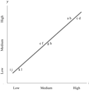
values of 𝑥, which represents a necessary and sufficient condition (Shering, Korhonen-Kurki and Brockhaus, 2013; Woodside, 2013; González-Velasco, González-Fernández and Fanjul-Suárez, 2017). While a necessary condition requires always the presence of a given factor for the occurrence of the outcome (for instance, factors that have to be presented if a media leads to a positive brand attitude), the sufficient condition means that whenever a given factor occur, the outcome will also occur (for instance, a specific set of attributes that together lead to a positive brand attitude), although the outcome can be achieve as a result of another factor (Shering, Korhonen-Kurki and Brockhaus, 2013; Mattke, Muller and Maier, 2019; Mello, 2019). The symmetrical effect can be represented as the Figure 1.
2 The net effect corresponds to the impact of each potential independent variable on the dependent variable after
the segregation of the influence of others independent variables on the dependent one (Woodside, 2013).
From Classical Regression Analysis to Qualitative Analysis: A Share Price fsQCA Empirical Application
10
However, the empirical evidences show that symmetrical effect does not fully fit the reality. So, the symmetrical effect is considered as a weakness of RA since this kind of analysis assumes either a symmetric relationship between the dependent and independent variable or a net effect of the independent variables on the dependent one. In fact, the reality shows that the asymmetrical effect4 is more common than the
symmetrical one (Woodside, 2014).
One type of asymmetrical effect is a sufficient but not necessary relationship, meaning that high values of 𝑥 are sufficient to achieve high values of 𝑦 but is not necessary since high
4 Asymmetric relationship has a correlation between 0.3 and 0.7 (Woodside, 2013).
0 1 2 3 4 5 6 7 8
1Low Medium High 2 3 4 5 6 7
Lo w Me di um H ig h a b c d e f g h i j k l 𝑦 𝑥
Figure 1: A symmetrical relationship between 𝑥 and 𝑦
Source: adapted from Wu et al. (2014)
0 1 2 3 4 5 6 7 8
1Low Medium High 2 3 4 5 6 7
Lo w M ed iu m H ig h a b c d e f g h i j k l 𝑦 𝑥
Figure 2: An asymmetrical relationship between 𝑥 and 𝑦 (sufficient but not necessary condition)
11
values of 𝑦 can be obtained with low values of 𝑥 or a given set of 𝑥 (Woodside, 2013; Wu et al., 2014; Mello, 2019). The Figure 2 represents the above-mentioned condition. Another type of asymmetric relationship can occur when high values of 𝑥 results not only in high values of 𝑦 but also in low values of 𝑦 (insufficient but necessary condition) (Wu et al., 2014).
In addition, while symmetric tests take into account the cause effect of high (low) values of 𝑥 on high (low) values of 𝑦, asymmetric tests consider any cause effect, either the effect of low (high) values of 𝑥 on high (low) values of 𝑦 or the effect of high (low) values of 𝑥 on high (low) values of 𝑦 (Woodside, 2014).
(iii) Linear relationship
The multiple regression analysis undertakes that the relationship between dependent and independent variables is linear and well explained by the square of correlation coefficient in case of simple regression (𝑅%). Nevertheless, the reality shows the opposite path (McClelland, 1998).
Other limitation of RA is related to the matrix algebra, as stated by Woodside (2013) and Wu et al. (2014). Moreover, these authors concluded that a Boolean algebra can contribute to mitige some issues mentioned above, through testing the relationships among indepedent variables as well as solving the symmetrical effect issue. This can be achieved by the Complexity Theory (hereinafter, CT), useful to go beyond the dominant logic of RA (Woodside, 2014) and to be applied in accounting, consumer research, finance, management and marketing (Woodside, 2013).
Additionally, in many social science applications, the estimators are not unbiased under assumptions LR.1 through LR.4 since ommitted factors in the error term are often correlated with the independent variables, known by endogeneity, and then the error term has not zero mean (Wooldridge, 2014).
Despite these limitations, RA should not be avoided but carefully used. In case of falling out its scope or abilities, RA should preferably be substituted by an adequate tool.
2.3. Complexity Theory
The CT considers that RA, as dominant logic, lacks objectivity in what respects to the use of independent variables and the challenge of hypothesis approaches (Armstrong, Brodie and Parsons, 2001). This theory accepts the nonlinear relationship between variables, since the cause effect of huge changes can produce different results (Woodside, 2014). On this way, the CT evaluates if the relationship among variables depends on the complex antecedent conditions (Wu et al., 2014).
From Classical Regression Analysis to Qualitative Analysis: A Share Price fsQCA Empirical Application
12
Therefore, several authors consider the reality too complex to disregard the dynamic, stochastic and nonlinear processes, considering the RA as a poor tool to fit the reality. Hence, a configural analysis is needed to estimate and to describe multiple realities because the simplicity of RA is not sufficient (Woodside, 2014).
Woodside (2014) and González-Velasco, González-Fernández and Fanjul-Suárez (2017) defined the tenets of the CT to mitigate the lack of rigor in order to formalise it. Thus, the CT is defined under six tenets, as follows:
Tenet T.1
Asymmetry principle: insufficient but necessary condition
A singular independent variable may be necessary, although it is mostly insufficient for predicting the value of the dependent variable.
Tenet T.2
Recipe principle
Two or more independent variables are sufficient for high values of the dependent variable.
Tenet T.3
Equifinality principle: sufficient but not necessary condition
A model that is sufficient is not necessary since another independent variable or a combination of independent variables can achieve the same results.
Tenet T.4
Causal asymmetry principle
A rejection does not mean the opposite situation of acceptance.
Tenet T.5
Relationship between independent variables
The presence of a given independent variable can positively or negatively influence the dependent variable depending on the presence or absence of another independent variable(s).
Tenet T.6
Non-perfect correlation
In a set of independent variables, that is relevant for the occurrence of the dependent variable, not all of them are individually significant for the result. As a result, the correlation is always less than 1.
Tenet T.7
Exemptions to the non-perfect correlation
The CT assumes the possibility of the existence of high values of 𝑥 that predict high values of 𝑦 as an exception.
13
2.4. Qualitative comparative analysis
Along different type of qualitative researches (Bansal, Smith and Vaara, 2018), Qualitative Comparative Analysis (hereinafter, QCA) is a methodological tool that mitigates the weaknesses of RA and respects the tenets of CT, being a real alternative to the dominant logic. Despite the name, QCA is not a qualitative method but a mix of qualitative5 and quantitative6
methodologies (Ragin, 2008; Mello, 2019). In addition, QCA is an approach since reflects better the social behaviour, the social thinking and the complexity of the reality. Nevertheless, several scientists and researchers use both approaches (i.e., RA and QCA) or other instruments, in order to get a better performance for their investigations (Shering, Korhonen-Kurki and Brockhaus, 2013). According to Berger and Kuckertz (2016), despite the application of QCA for political science and sociology as an accurate method, QCA has been increasingly used in business and management researches. In particular, QCA is preferentially applied at country level and organizational level analysis.
In addition, QCA is an asymmetric model that indicates all the cases or almost of them with relatively high values of the dependent variable that are caused by relatively high values of independent variable(s) (Wu et al., 2014). In fact, neither a simple nor a multiple regression are necessary to achieve high values of 𝑦. Rather than the net effects of independent variables on the dependent one foreseen by RA (Ragin, 2008), multiple combinations between independent variables are more relevant for the results. To sum up, QCA assumes that the dependent variable depends on how different independent variables are related, rather than the importance of each individual one (Woodside, 2013; Ordanini, Parasuraman and Rubera, 2014; Mattke, Muller and Maier, 2019).
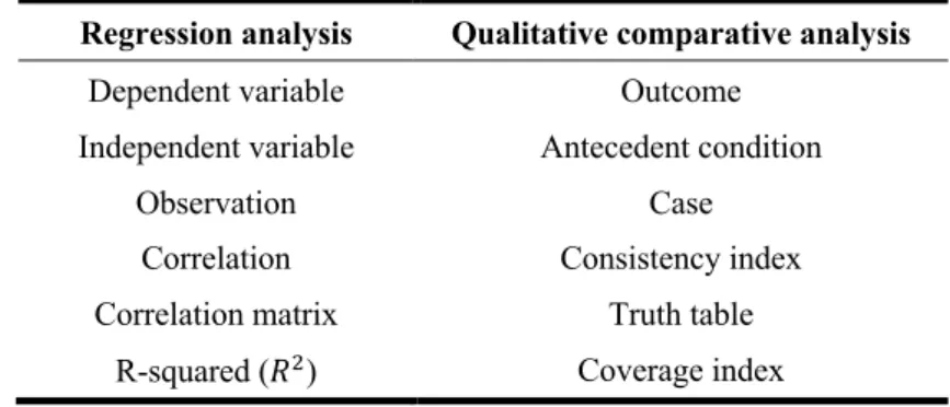
Compared to RA, some nomenclature needs to be adjusted in QCA, which will be used hereinafter, as follows.
Figure 3: Comparison between RA and QCA nomenclatures
Regression analysis Qualitative comparative analysis
Dependent variable Outcome Independent variable Antecedent condition
Observation Case Correlation Consistency index Correlation matrix Truth table
R-squared (𝑅%) Coverage index
5 Qualitative means non-numerics and inductive theorizing (Bansal, Smith and Vaara, 2018). 6 Quantitative means numerics that can be manipulated (Bansal, Smith and Vaara, 2018).
From Classical Regression Analysis to Qualitative Analysis: A Share Price fsQCA Empirical Application
14
One advantage of QCA is its application on small/intermediate data size since it provides more accurate results, even if the data is small for a quantitative analysis, such as RA, or big for a qualitative analysis, such as QCA (Shering, Korhonen-Kurki and Brockhaus, 2013; Berger and Kuckertz, 2016). 2.4.1. fsQCA, a kind of QCA
Since QCA treats the conditions in a set way, this methodology is also known by set-theoretical method. One kind of QCA approaches is express the conditions in a binary way, such as dummy variables, called Crisp-set Qualitative Comparative Analysis (Ragin, 2008; Shering, Korhonen-Kurki and Brockhaus, 2013). This QCA classifies the conditions in a gradual scale, called by crip-set, such as “absence” or “presence”, where the 0 means absence and 1 means presence. However, it is possible to measure the conditions with more exactness, like “absence”, “more absence”, “more presence” and “presence”, achieving more precision and discrimination. This approach is called Fuzzy-set Qualitative Comparative Analysis (fsQCA) and it is considered as an extension of the Crisp-set Qualitative Comparative Analysis since it allows the researchers to grade set memberships in fuzzy-sets that range between 0 and 1, where 0 corresponds to “absence”, 1 to “presence” and somewhere between these values will be “more absence” and “more presence” (Rihoux and Regin, 2007; Ragin, 2008; Shering, Korhonen-Kurki and Brockhaus, 2013; Mello, 2019).
The definition of the limits for a fuzzy-set and the consequent attribution of a scale from 0 to 1 is based on judgment and own knowledge of the researcher and/or based on empirical evidence and statistical data (Ragin, 2008; Shering, Korhonen-Kurki and Brockhaus, 2013).
Figure 4: Kind of fuzzy-sets
Crisp-set Three-value fuzzy-set Four-value fuzzy-set Six-value fuzzy-set Continuous fuzzy-set
𝑥H= 1.0
fully in 𝑥fully in H= 1.0 𝑥Hfully in = 1.00
𝑥H= 1.0
fully in 𝑥H= 0.8
mostly but not fully in 𝑥H= 0.6
More or less in 𝑥H= 0.4
More or less out 𝑥H= 0.2
mostly but not fully out 𝑥H= 0.0 fully out 𝑥H= 1.0 fully in 𝑥H= 0.75
more in than out
𝑥H= 0.25
more out than in
0.5 < 𝑥H< 1.0
more in than out 𝑥H= 0.5
Neither fully in nor fully out
𝑥H= 0.5
cross-over 0.0 < 𝑥H< 0.5
more out than in 𝑥H= 0.0
15
Ragin (2008) clearly stated different types of fuzzy-sets through the figure above.
In the light of the above-mentioned, fsQCA is more than a qualitative approach since it bridges the qualitative to the quantitative approach. Therefore, the QCA is also considered as a quantitative method due to the numerical information between these qualitative states, in particular regarding the continuous fuzzy-set (Ragin, 2008; Mello, 2019).
Many authors, such as González-Velasco, González-Fernández and Fanjul-Suárez (2017) and Fotiadis (2018), generally defined three breakpoints values to scale the fuzzy-sets: 0.95 to represent the full membership since original values cover 95% of data values, 0.50 to represent the cross-over and 0.05 to represent the full non-membership since original values cover 5% of data values.
In addition, fsQCA aims at analysing of casual sufficiency to evaluate which antecedent conditions are sufficient to obtain the outcome. On one hand, the sufficiency is verified if the cause is a subset of the outcome, since the membership score of the cause is less or equal than its membership score in the outcome. On the other hand, the necessity is verified if the outcome is a subset of the cause. In this case, the membership score of the outcome is less or equal than the membership score in the cause (González-Velasco, González-Fernández and Fanjul-Suárez 2017; Mello, 2019).
QCA uses the Boolean algebra to represent the operations on fuzzy-sets. The three most common operations are the negation, the logical or and the logical and. As the name suggests, the former is the opposite of the membership score and is represented as ~ or with lowercase7.
In case of a crisp-set, the negation of a score of 1 is 0 and vice-versa, while with a fuzzy-set the negation is achieved through the following equation:
~𝐴 = 1 − 𝐴 (9)
In its turn, the logical or, represented as + or ∪, refers to the union of two or more sets and corresponds to the maximum value across sets. On contrary, the logical and is expressed by ∗ or ∩ and refers to the intersection of sets. Thus, the logical and corresponds to the minimum value across sets (Ordanini, Parasuraman and Rubera, 2014; Mello, 2019).
From Classical Regression Analysis to Qualitative Analysis: A Share Price fsQCA Empirical Application
16
2.4.2. Methodology of QCA
Ordanini, Parasuraman and Rubera (2014) referred that the application of QCA involves four steps:
(i) Property space
The definition of the property space consists in determining all possible combinations of antecedent conditions that lead to the occurrence of the outcome.
(ii) Set-membership measures
This step, also known by calibration, consists in transforming the original variables, expressed in a continuous scale, into sets in order to make a range from 0 to 1.
According to Longest and Vaisey (2008), the combinations defined in the property space should also include the negation of each antecedent condition. By this way, all cases have some degree of membership measure in every combinations of antecedent conditions, although each case has a membership measure higher than 0.50 in only one combination, called best-fit case.
(iii) Consistency in set relations
The third step consists in assessing the combinations that acts as sufficient conditions for the occurrence of the outcome, called by consistent cases.
As reported by González-Velasco, González-Fernández and Fanjul-Suárez (2017), consistency is one of the key concepts related to QCA, is equivalent to correlation coefficient and can assessed through the proportion of consistent cases, computed as follows. 𝐶𝑜𝑛𝑠𝑖𝑠𝑡𝑒𝑛𝑐𝑦 (𝑥H ≤ 𝑦H) =∑ [min(𝑥H; 𝑦H)] ] H ∑ 𝑥] H H (10)
where 𝑥H represents the antecedent conditions, 𝑦H the outcome condition and 𝑛 the number of observations.
A condition is considered as sufficient when its consistency shall statistically exceed a given threshold. Usually, researchers consider a consistency threshold of 0.80 to treat the condition as sufficient (Longest and Vaisey, 2008; Ordanini, Parasuraman and Rubera, 2014; Mattke, Muller and Maier, 2019).
(iv) Logical reduction
The last step consists in assessing the sufficient conditions and eliminating the unneeded elements since some of them are indifferent to achieve the outcome. Hence, it is used another key concept for QCA, the coverage measure (Velasco,
González-17
Fernández and Fanjul-Suárez, 2017), which is computed in order to evaluate the relevance of the sufficient conditions.
𝐶𝑜𝑣𝑒𝑟𝑎𝑔𝑒 (𝑥H ≤ 𝑦H) =∑ [min(𝑥]H H; 𝑦H)] ∑ 𝑦]H H
(11)
where 𝑥H represents the antecedent conditions, 𝑦H the outcome condition and 𝑛 the number of observations.
According to González-Velasco, González-Fernández and Fanjul-Suárez (2017), coverage is equivalent to variance in RA.
2.4.3. An empirical example
Several studies have been performed over the years and a lot of researchers have concluded about the useful of QCA.
In their research, Ordanini, Parasuraman and Rubera (2014) studied the impact of innovativeness on new hotel service adoption, in particular which combinations of attributes lead to the adoption of the service, since empirical evidences had revealed inconclusive. Through the comparison between RA and QCA, these researchers accomplished that the net effects are too simpler to represent the reality. So, the studied concluded that different combinations of antecedent conditions act as sufficient conditions for the adoption of a new service.
These authors used the attributes described below as antecedent conditions for the occurrence of new service adoption, that were measured as a degree of perception and were collected through a questionnaire:
Relative advantage
[𝐴𝑑𝑣]
The new service is perceived as better than other alternatives.
Complexity
[𝐶𝑜𝑚𝑝𝑙]
Complexity corresponds to the perception of how the new service is hard to understand and then an additional effort is needed to adopt the service (for instance, learning lessons or trainings).
Meaningfulness
[𝑀𝑒𝑎𝑛]
From Classical Regression Analysis to Qualitative Analysis: A Share Price fsQCA Empirical Application
18
Novelty
[𝑁𝑜𝑣]
The new service is perceived as incongruent, compared with other alternatives, and as uncertain, regarding the consequence of the adoption.
Coproduction requirements
[𝐶𝑜𝑝𝑟]
Coproduction requirements reflects the organisational choice made by the service provider in which the customer is involved in the service.
Through the use of QCA, the study concluded that the combinations of attributes8 that are
sufficient9 to achieve the new service adoption are:
(i) 𝒎𝒆𝒂𝒏 ∗ 𝒄𝒐𝒎𝒑𝒍 ∗ 𝑨𝑫𝑽 ∗ 𝑪𝑶𝑷𝑹
The new service is seen as a good alternative, non-complex and with a high degree of coproduction, although it is not immediately perceived as useful.
(ii) 𝑵𝑶𝑽 ∗ 𝑨𝑫𝑽 ∗ 𝒄𝒐𝒑𝒓
The adoption is induced by the perception of the new service as a good alternative and as novel but requiring low level of coproduction.
(iii) 𝑵𝑶𝑽 ∗ 𝑴𝑬𝑨𝑵 ∗ 𝑨𝑫𝑽
The adoption of the new service can be induced when customers perceive it as being novel, useful and a good alternative.
Taking into account these combinations, the researchers concluded that relative advantage is a necessary but not sufficient condition for the occurrence of the new service since its presence can induce the adoption, however individually presence does not mean the adoption.
Moreover, the antecedent conditions novelty, non-complexity and meaningfulness are neither necessary, nor sufficient conditions since are not present in the three combinations. In addition, meaningfulness can be either absent (first combination), irrelevant (second combination) or present (third combination) for the occurrence of the new service adoption and non-complexity and novelty can be either present (first combination in case of non-complexity and second and third combinations in case of novelty) or irrelevant (first combination in case of novelty and second and third combinations in case of non-complexity) for the occurrence of the new service adoption.
8 Lowercase and uppercase correspond to the absence and presence of the attributes, respectively. 9 These three combinations explain 78% of the adoption of the new service (total coverage measure).
19
Through the using of RA, researchers concluded that, regarding individual effects, relative advantage and novelty have positive effect on the service adoption (𝛽••‘ = 0.50∗ and 𝛽’“‘ = 0.20*), being the former the most important predictor. On contrary, complexity and
coproduction show negative effects (𝛽”“•–— = −0.20* and 𝛽
”“–˜ = −0.18*). Additionally, meaningfulness is not relevant as a predictor since it is not statistically significant10. In what
respects to interaction effects, RA reveals the following models as predictors of the new service adoption: (i) Model 1 𝐴𝑑𝑜𝑝𝑡𝑖𝑜𝑛H = 𝛽)𝑁𝑜𝑣 ∗ 𝑀𝑒𝑎𝑛 ∗ 𝐶𝑜𝑝𝑟H+ 𝛽%𝑀𝑒𝑎𝑛 ∗ 𝐶𝑜𝑚𝑝𝑙 ∗ 𝐴𝑑𝑣H+ + 𝛽=𝑀𝑒𝑎𝑛 ∗ 𝐴𝑑𝑣 ∗ 𝐶𝑜𝑝𝑟H+ 𝑢H (12) (ii) Model 2 𝐴𝑑𝑜𝑝𝑡𝑖𝑜𝑛H = 𝛽)𝑀𝑒𝑎𝑛 ∗ 𝐶𝑜𝑚𝑝𝑙 ∗ 𝐴𝑑𝑣 ∗ 𝐶𝑜𝑝𝑟H + 𝑢H (13)
The highest order of significance is for 𝑀𝑒𝑎𝑛 ∗ 𝐶𝑜𝑚𝑝𝑙 ∗ 𝐴𝑑𝑣 ∗ 𝐶𝑜𝑝𝑟, which corresponds to the first combination of attributes that are sufficient for the new service adoption revealed by QCA, described above.
Comparing the results obtained with both approaches, the authors concluded that RA revealed small size effects of the independent variables and did not detect the trade-off effects between them while QCA captured the sufficient and necessary conditions and the relationships between the antecedent conditions for the occurrence of the new service adoption even if some of them had to be absent.
2.5. Share price conditions: An application
This study is based on an investigation of potential factors that influence the share price of listed companies. In fact, several studies have been developed in order to find the variables that can trigger the share price of enterprises, most of them related to accounting information, although some of results have not been conclusive and have shown contradictory results. Moreover, all papers used the 𝑂𝐿𝑆 regression to figure out the contributions for the share price variations.
Menaje (2012), Lestari (2017), Nautiyal and Kavidayal (2018) and Hung, Ha and Binh (2018) assessed the impact of some factors on the share price of companies listed in Asian stock
* 𝑝 < 0.05. 10 𝑝 = 0.24.
From Classical Regression Analysis to Qualitative Analysis: A Share Price fsQCA Empirical Application
20
markets, such as Philippian, Indonesia, Indian and Vietnam, respectively. It is worth mentioning that only Menaje (2012) used a one-year data (2009), while the others used a multi-year data to perform their analysis (2012-2014, 1995-2014 and 2006-2016, respectively). In fact, the findings revealed inconsistent results in what respects to the influence of the earning per share factor (hereinafter, 𝐸𝑃𝑆) on the share price (Menaje, 2012; Nautiyal and Kavidayal, 2018). While Menaje (2012) concluded about the strong positive correlation with the share price, Nautiyal and Kavidayal (2018) found a poor relationship between 𝐸𝑃𝑆 and the share price. Also, contradictory outcomes were verified for the influence of the return on asset factor (hereinafter, 𝑅𝑂𝐴) because whilst Hung, Ha and Binh (2018) revealed a positive correlation, Menaje (2012) concluded about a weak negative relationship.
In his turn, Lestari (2017) verified that the retained earnings to total assets have a positive impact on the share price, not only individually, but collectively too, all together with sales growth and sales to current assets. Similarly, positive relations with the share price were also found for the economic value added (Nautiyal and Kavidayal, 2018), the company size (measured by the net revenue), the current ratio (measured by short-term assets over short-term liabilities) and the accounts receivable turnover (measured by net revenue over receivables) (Hung, Ha and Binh, 2018). On contrary, Nautiyal and Kavidayal (2018) showed that dividend per share and dividend payout have a negative effect on the share price. Finally, Hung, Ha and Binh (2018) found that the capital structure, in particular the leverage level of the company (hereinafter, 𝐿𝐸), does not have any impact on the share price.
In a European research, Avdalovic and Milenkovic (2017) studied the share price conditions of companies listed in Serbian stock market, through a multi-year data (2010-2014). The results revealed that the book value per share (hereinafter, 𝐵𝑉𝑃𝑆) and 𝑅𝑂𝐴 had the major contribution for a positive variation of the share price. Additionally, 𝐿𝐸 and price to book ratio also provided positive contributions for the share price fluctuation, despite of a lower meaningful. On contrary, 𝐸𝑃𝑆 and the company size (measured by the assets) had a negative impact on the share price. Another factor that has been analysed in several researches, given its influence on the share price fluctuation, is the structure of corporate ownership, although the results still remain ambiguous. In fact, corporate governance has become one of the most discussed matter after the last financial crisis, which led several companies to the bankruptcy due to governance issues. However, the corporate ownership also assumes a huge importance considering a direct effect on corporate power in case of an ownership control. In the light of the above mentioned, it is important to assess the type of corporate ownership since each entrepise has a particular
21
structure: domestic ownership, foreigner ownership, diversified structure of ownership, qualified ownership, managers who have a stake, among others.
Vintila and Gherghina (2014), Alves, Canadas and Rodrigues (2015) and Jankensgard and Vilhelmsson (2018) performed their resourches in European countries, which assessed the impact of corporate ownership’s struture on the share price of companies listed in the stock markets of Romania, Portugal and Spain, and Swedeen, respectively. In general, the share price volatility increased with the number of relatively large shareholders and the portion of shares held by shareholders with stakes lower than 0.1% (Jankensgard and Vilhelmsson, 2018). However, Alves, Canadas and Rodrigues (2015) concluded that the biggest ownership had a negative impact on the share price. Although Vintila and Gherghina (2014) did not obtain statistical significant results regarding the influence of the large ownership, the results revealed that the second and third largest shareholders, as well as the sum of the three largest shareholders, were positively related to the share price volatility. On contrary, ownerships lower than 13.08% had negative influence on the share price volatility.
In addition, the positive effect of the first and fifth largest shareholder in an individual basis were verified by Alzeaideen and Al-Rawash (2014) in a study of enterprises listed in the Jordanian stock market. However, ElGhouty and El-Masry (2017) did not find any relationship between the ownership concentration and the stock return. These authores only concluded about a positive impact on the ex ante risk.
From Classical Regression Analysis to Qualitative Analysis: A Share Price fsQCA Empirical Application
22
3. Methodology
The comparison between RA and QCA is performed in the context of a business and management research, through a cross-sectional data that includes financial information about companies of 2016.
3.1. Sample characterization
The sample is composed by 𝟐𝟔𝟓 European listed companies, which are from the following countries: Austria, Denmark, Finland, France, Germany, Italy, Netherlands, Norway, Poland, Portugal, Russia, Spain, Sweden, Switzerland, Turkey and United of Kingdom.
First of all, the 2016 World’s Billionaires list is gathered from the Forbes website. The billionaires who have a stake in European listed companies are selected from this list (in a total of 89 billionaires) and the respective companies are added to the sample. It is worth mentioning that Forbes provides a real time list of the world’s billionaires, which is updated every day: while the value of public holdings is updated every five minutes, when the correspondent stock markets are open, the billionaires’ wealthiness tied to private companies are updated once a day. If a billionaire holds an ownership on a company that represents more than 20% of his/her net worth, the value is adjusted following the industry or region market index.
Secondly, other European listed companies are added to the sample taking into account the same sector/industry and similar size, but without any relationship with the billionaires from the Forbes’ list (in a total of 176).
The description of the sample is attached in Annex 1.
3.2. Variables description
The data is composed by the following 8 variables/conditions: billionaire (𝐵𝐼), price per share (𝑃𝑃𝑆), book value per share (𝐵𝑉𝑃𝑆), earnings per share (𝐸𝑃𝑆), leverage level (𝐿𝐸), return on asset (𝑅𝑂𝐴), size of company (𝑆𝑍) and cashflow from operations on asset (𝐶𝐹𝑂𝐴). It is worth mentioning that 𝐵𝐼𝐿 is a dummy variable that is defined as a binary variable equal to 1 if a company is owned by a billionaire and 0 otherwise.
The definition and information11 regarding these variables are described in Annex 2 and Annex
3, respectively.
23
3.2.1. Potential dependent variables / outcome conditions
In this data, the dependent variable or the outcome (in case of RA or fsQCA, respectively) is 𝑃𝑃𝑆, which is measured in Euros and refers to the price of a single share of a number of saleable stocks issued by a listed company. Therefore, this research aims at assessing the independent variables that have impact on the share price of a European listed company and the antecedent conditions that leads to a higher score of the share price, through the application of RA and QCA, respectively.
3.2.2. Potential independent variables / antecedent conditions
The potential independent variables / antecedent conditions are the remaining ones that are referred in several researches as factors that can influence 𝑃𝑃𝑆.
While the variables 𝐵𝑉𝑃𝑆 and 𝐸𝑃𝑆 are measure in Euros, 𝐿𝐸, 𝑅𝑂𝐴, 𝐶𝐹𝑂𝐴 and 𝑆𝑍 are percentages since refers to financial ratios, except the variable 𝑆𝑍 that corresponds to the natural logarithm of company’s assets.
3.3. Hypotheses
The hypotheses intend to achieve the objectives of this thesis and therefore verify which factors defined in previous section have more impact on the share price as well as compare both methodologies used. For that purpose, the hypotheses are supported by the literature review. In this sense, their drafting takes into account the relevant papers on these matters.
Hypothesis 1
None antecedent condition regarding accounting information is sufficient or necessary for a high score of 𝑃𝑃𝑆 (concluded through QCA).
The first hypothesis to be tested intends to demonstrate that none accounting information factor, such as 𝐵𝑉𝑃𝑆, 𝐸𝑃𝑆, 𝐿𝐸, 𝑅𝑂𝐴, 𝑆𝑍 or 𝐶𝐹𝑂𝐴, contributes for 𝑃𝑃𝑆, considering that several studies, mostly conducted through RA, are not conclusive regarding the factors that have significant impact on 𝑃𝑃𝑆. The test is performed though the QCA.
Hypothesis 2
Billionaires that hold a stake in a company do not have positively or negatively influence on the company’s 𝑃𝑃𝑆 (concluded through RA), neither produces a high score of 𝑃𝑃𝑆 (concluded through QCA).
The second hypothesis aims at verifying the particular impact of the ownership structure, in particular if a company is owned by a billionaire, on 𝑃𝑃𝑆. This hypothesis is related to this
From Classical Regression Analysis to Qualitative Analysis: A Share Price fsQCA Empirical Application
24
specific factor because does not exist enough studies about this subject, neither using RA, nor QCA. Due to this fact, this hypothesis is tested through both methodologies, RA and QCA.
Hypothesis 3
Overall, QCA provides similar results to RA.
The third hypothesis to be tested proposes to corroborate some authors’ point of view that claim the complementary between both kind of analysis. The test will be conducted through the comparison of the results obtained from both RA and QCA.
Hypothesis 4
Both RA and QCA do not produce univocal results with previous researches in what respects to the share price conditions.
Several researches about these matters have not produced conclusive results. Additionally, some authors argue that RA and QCA should be used as complement tools of each other, as previously referred. Due to these, the fourth hypothesis intends to report that the results provided by both approaches are ambiguous, when the literature review is considered.
3.4. Empirical application
The empirical strategy adopted in this research is the following. Firstly, the fsQCA software is used to estimate the model. For that, a definition of the property space is needed based on the knowledge and judgment. Moreover, the calibration is needed since the data is analysed through sets, in particular fuzzy-sets. Additionally, the Boolean algebra is applied and the subset relationships assessed. The final step is to reduce the sufficient combinations by deleting redundant elements.
In order to compare the results from the previous approach, a data analysis through a classical software is required. For that, the Eviews software is used.
3.4.1. Qualitative comparative analysis
As referred in the literature review section, the first step in the fsQCA methodology is to define the property space. For that purpose, all antecedent conditions in Section 3.2.2. are considered since they are drivers that aim at explaining the outcome condition. After that, the non-best-fit cases are excluded from the property space, following the methodology used by some authors. In the second place, the original measures of the conditions are replaced by the set-membership measures of fsQCA methodology, through a process known by calibration. Therefore, the original scale of values is transformed into a fuzzy-set scale. For that purpose, three breakpoints
25
values are defined according to the literature review: 0.95 to represent the full membership, 0.50 to represent the cross-over and 0.05 to represent the full non-membership.
Third, the consistency in set relations and the logical reduction are assessed in the truth table, which is extracted from the fsQCA software. For that purpose, it is only considered the combinations of antecedent conditions that have a consistency value higher than 0.80. After that, the truth table solution is generated in order to disclose the conclusions provided by QCA.
3.4.2. Regression analysis
In order to explain the influence of accounting information and ownership structure on company’s 𝑃𝑃𝑆, an econometric analysis is conducted. Thus, it is possible to obtain a model that explain 𝑃𝑃𝑆 as far as possible. After this, the model is tested.
The most accurate model is found out by adding the potential independent variables to the model and decide about their statistical significance by looking for the 𝑡-test as well as for the adjusted 𝑹𝟐 (𝑅$%) and the information criteria.
As describe in the Section 2.1.2., when variables are added to the model it is possible to verify if they are statistically significant by looking for the raise of the 𝑅$%. Unless this coefficient increases, the variables are not statistically significant to explain the dependent variable. On contrary, smaller values of the information criteria means that the model is more reliable.
Firstly, the potential independent variables are individually added and, if 𝑅$% increases and the information criteria decreases, the decision is to keep them in the model. Aiming at improving the model, squares of the independent variables and the combination between dummy - non-dummy variables are also included. Notice that non-dummy - non-dummy combinations are excluded since they do not have great economic and financial interpretation. Once again, variables are excluded if their introduction led a negative impact on 𝑅$% or increases the information criteria.
Secondly, the relevance of the independent variables is assessed. Hence, if the respective parameter is not statistically different from zero (𝑝 − 𝑣𝑎𝑙𝑢𝑒 > 𝛼), the independent variable is not relevant to explain the dependent one and is removed as well.
Finally, if a new independent variable is added to the model and makes irrelevant another independent variable already included, it is necessary to find the combination that offers a greater 𝑅$% and a lower information criteria.