2019
UNIVERSIDADE DE LISBOA FACULDADE DE CIÊNCIAS DEPARTAMENTO DE INFORMÁTICA
Automatic Detection of Anomalous User Access Patterns to
Sensitive Data
Mariana Galhardas Pina
Mestrado em Informática
Dissertação orientada por:
Acknowledgements
I would like to thank DCY department at Altice for receiving me with open arms and for all the support given. Special thank you to Eng. José Alegria for the opportunity and guidance throughout the project. Another special thank you to Ricardo Ramalho for the guidance, help and motivation as a team leader in which I was integrated. Thank you to Professor Pedro Ferreira for accepting to be my advisor, for the time spent and all the guidance throughout this project.
i
Resumo
Esta dissertação foi realizada por uma aluna da Faculdade de Ciências da Universidade de Lisboa, com licenciatura em Matemática Aplicada e atualmente a frequentar o mestrado em Informática. A proposta desta dissertação veio do departamento de Cibersegurança (DCY) da Altice Portugal (MEO) e a área de especialização é aprendizagem máquina (machine learning).
Nos últimos anos, especialmente em grandes organizações, o roubo de informação confidencial tem vindo a ser uma problemática cada vez maior. Este tipo de ataque tem, normalmente, duas origens distintas: colaboradores maliciosos ou malware instalado, possivelmente proveniente de um ataque de phishing. No entanto, atividade anónima sem intenção maliciosa também pode ser relevante, pois pode ser um indicador de um uso incorreto de recursos da rede ou de uma violação de política.
Este trabalho aborda este problema de segurança através da aplicação de técnicas de aprendizagem máquina com o objetivo de detetar anomalias, correspondentes a atividades ilícitas, no registo de acessos a dados de informações de clientes e/ou meta-dados feitos por utilizadores de backoffice,. Um dos objetivos é a distinção dessas anomalias, mais concretamente, a classificação dessas situações de roubo de informação confidencial em diferentes tipos, para que as pessoas responsáveis pela parte posterior da investigação interna saibam o que devem procurar. Para além disso, procuramos reduzir ao máximo o número de falsos positivos, mantendo um grau de deteção elevado.
Anteriormente, a empresa realizou um projeto com o mesmo objetivo final, no entanto, com uma metodologia completamente distinta. Nesse projeto foram aplicados métodos de estatística descritiva e heurísticas simples para a deteção de anomalias, tendo sido intitulou de Cuscos. O projeto Cuscos detetou um número bastante elevado de anomalias (1800), contudo identificou-se um número muito alto de possíveis falsos positivos, tendo sido uma problemática. Adicionalmente, a impossibilidade de distinguir os diferentes tipos de atividade ilícita, constituiu um obstáculo, tendo, assim, cada anomalia que ser estudada individualmente para que se descobrisse a sua causa. Como se pode ver pelos objetivos acima descritos, este projeto procura solucionar estas dificuldades.
ii
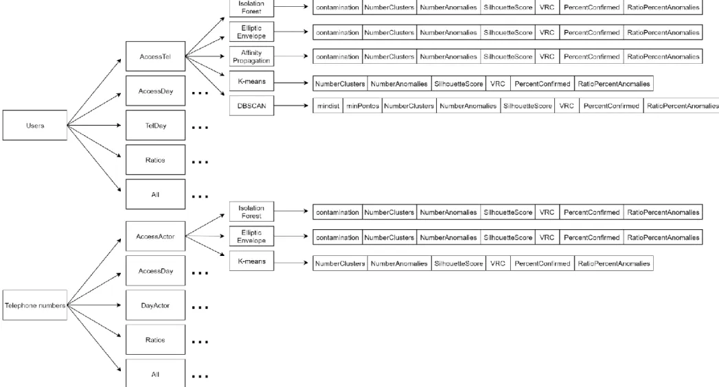
Primeiro, fez-se uma caracterização estatística dos dados, onde se decidiu que características (features) dos dados originais deviam ser criadas ou extraídas para a construção de conjuntos de dados (datasets) e, posteriormente, para a aplicação dos algoritmos de aprendizagem máquina (machine learning) escolhidos. Nesta, foram consideradas duas abordagens: uma em ordem aos utilizadores e outra direcionada aos números de telefone. Como tal, foram criados dois conjuntos de dados, um para cada abordagem. De seguida, executaram-se os procedimentos necessários de pré-processamento e normalização dos dados. Finalmente, foram aplicados algoritmos de agrupamento de dados e deteção de anomalias aos conjuntos de dados criados. Os algoritmos de agrupamento de dados considerados foram: k-means, DBSCAN e affinity
propagation; e os algoritmos de deteção de anomalias escolhidos foram: elliptic envelope e isolation forest. Para determinar os parâmetros adequados de cada um desses
algoritmos, foram definidos intervalos de parâmetros e criadas tabelas de pontuação com os resultados obtidos a partir da aplicação desses algoritmos com as diferentes combinações de parâmetros. Para obter resultados específicos para diferentes perspetivas analíticas, além de serem aplicados em todo o conjunto de dados construído, os algoritmos também foram aplicados a diferentes combinações de algumas de suas características.
Tendo em conta que as anomalias finais são referentes a utilizadores, os resultados da abordagem dos números de telefone tiveram de ser convertidos, isto é, os utilizadores que acederam aos números de telefone considerados como anomalias pela aplicação dos algoritmos substituíram os números de telefone, sendo, assim, os utilizadores as anomalias consideradas. Em cada abordagem, foi escolhido um método de ensemble para decidir quais dos utilizadores detetados seriam considerados anomalias finais. Finalmente, obtiveram-se os resultados finais através de um ensemble por união do conjunto de resultados de ambas as abordagens e, posteriormente, criaram-se regras de decisão para classificar as anomalias em diferentes categorias.
Os resultados finais cumpriram todos os objetivos: detetaram-se anomalias relevantes de situações correspondentes a acessos ilícitos, reduziu-se o número de falsos positivos e cada anomalia detetada está classificada consoante o tipo de comportamento que representa.
Palavras-chave: aprendizagem automática, cibersegurança, roubo de informação, deteção de anomalias
iii
Abstract
In recent years, especially in large organizations, the theft of valuable information has increasingly become a major problem.
This project focuses on users access to information related to customer telephone numbers inside a telecom company. The objective is to, through machine learning techniques, detect illicit accesses to this information, focusing on those likely to match information theft actions.
First, we made a statistical characterization of the data. Decided which features should be created or extracted from data to build the necessary datasets (two different approaches) to apply the algorithms, and then the required pre-processing and normalization procedures were executed. Finally, we applied clustering and anomaly detection algorithms to detect anomalies in the datasets. The algorithms considered were: k-means, DBSCAN, affinity propagation clustering methods, elliptic envelope and isolation forest anomaly detection methods. To determine optimal parameters for the algorithms on this data, parameter ranges were defined and score tables were created with the results obtained from different combinations of parameters. To obtain specific results for different analytic perspectives, besides being applied on the entire datasets built, the algorithms were also applied to different combinations of some of their features. Finally, after the algorithms application, ensemble methods were chosen and decision rules were created to classify the anomalies in different categories.
The final results met all objectives. Relevant anomalies were detected in situations corresponding to illicit accesses, the number of false positives was reduced and each detected anomaly is classified according to the type of behavior it represents.
v
Table of Contents
Chapter 1 Introduction ... 1 1.1 Motivation ... 1 1.2 Objectives ... 2 1.3 Document Structure ... 2Chapter 2 Related Work... 3
2.1 Previous Studies ... 3
2.2 Fundaments and Tools ... 5
2.2.1 Jupyter ... 5
2.2.2 Python... 5
2.2.3 Machine Learning ... 5
2.2.4 Clustering Algorithms ... 6
2.2.5 Anomaly detection algorithms ... 7
2.2.6 Evaluation Metrics ... 7
2.2.7 HIDRA ... 9
2.2.8 Docker ... 10
Chapter 3 Methodology ... 11
3.1 Data Study ... 13
3.1.1 Characterization of APPS-GPD dataset ... 15
3.2 Pre-processing ... 23 3.2.1 User Approach... 24 3.2.2 Telephones approach ... 26 3.2.3 Normalization ... 28 3.3 Anomalies ... 28 3.4 Algorithms ... 30 3.4.1 K-means ... 30 3.4.2 DBSCAN ... 31 3.4.3 Affinity Propagation ... 32
vi 3.4.4 Elliptic Envelope ... 32 3.4.5 Isolation Forest ... 33 3.5 Parameterization ... 34 3.6 Ensemble ... 39 3.7 Classification ... 40 3.8 Process Automation ... 41 Chapter 4 Results ... 43 4.1 User Approach ... 43 4.2 Telephone Approach... 53 4.3 Final Results ... 60
Chapter 5 Conclusions and Future Work ... 67
References ... 69
Appendix A ... 72
Appendix B – Users approach: Score Tables for perspective Ratios ... 73
Appendix C – Users approach: Score Tables for perspective AccessDays ... 77
Appendix D – Users approach: Score Tables for perspective AccessTel ... 81
Appendix E – Users approach: Score Tables for perspective TelDays ... 85
Appendix F – Users approach: Score Tables for perspective All ... 89
Appendix G – Telephones approach: Score Tables for perspective Ratios ... 93
Appendix H – Telephones approach: Score Tables for perspective AccessDay .... 95
Appendix I – Telephones approach: Score Tables for perspective AccessActor ... 97
Appendix J – Telephones approach: Score Tables for perspective DayActors ... 99
Appendix K – Telephones approach: Score Tables for perspective All ... 101
vii
List of Figures
Figure 1- Project methodology ... 12
Figure 2- Distribution of the number of times each actor made an access ... 15
Figure 3- Distribution of the number of times each actor made an access without extreme cases ... 16
Figure 4 - Distribution of the number of times each actor, which made less than 1000 accesses, made an access ... 16
Figure 5- Distribution of the number of different days each actor made an access 17 Figure 6- Distribution of the number of times each user, that made more than 10000 accesses, made an access ... 18
Figure 7- Distribution of the number of times each user, which made between 1000 and 10000 accesses, made an access ... 18
Figure 8-Distribution of the number of times each user, which made less than 1000 accesses, made an access ... 19
Figure 9-Distribution of the number of different days each user made an access .. 19
Figure 10-Distribution of the number of times each telephone number, which was accessed more than 1000 times, was accessed ... 20
Figure 11-Distribution of the number of times each telephone number, which was accessed between 10 and 1000 times, was accessed ... 21
Figure 12-Distribution of the number of times each telephone number, which was accessed less than 1000 times, was accessed ... 21
Figure 13-Distribution of the number of different days each telephone number was accessed ... 22
Figure 14-Distribution of the number of times each application was used to access telephone numbers ... 22
Figure 15-Distribution of the number of different days each application was used to access telephone numbers ... 23
Figure 16- Explanation of score tables created for the parameterization optimization ... 35
Figure 17- Automation process architecture ... 41
Figure 18-Anomalies detected by Elliptic Envelope ... 44
viii
Figure 20-Anomalies detected by K-means ... 44
Figure 21- Anomalies detected by DBSCAN ... 44
Figure 22-Anomalies detected by Isolation Forest ... 44
Figure 23-Anomalies detected by Elliptic Envelope ... 45
Figure 24-Anomalies detected by DBSCAN ... 45
Figure 25-Anomalies detected by Affinity Propagation ... 46
Figure 26-Anomalies detected by Isolation Forest ... 46
Figure 27-Anomalies detected by K-means ... 46
Figure 28-Anomalies detected by Isolation Forest ... 47
Figure 29-Anomalies detected by K-means ... 47
Figure 30-Anomalies detected by DBSCAN ... 47
Figure 31-Anomalies detected by Elliptic Envelope ... 47
Figure 32-Anomalies detected by K-means ... 48
Figure 33-Anomalies detected by DBSCAN ... 48
Figure 34-Anomalies detected by Elliptic Envelope ... 48
Figure 35-Anomalies detected by Affinity Propagation ... 48
Figure 36-Anomalies detected by Isolation Forest ... 48
Figure 37-Anomalies detected by K-means ... 50
Figure 38-Anomalies detected by Affinity Propagation ... 49
Figure 39-Anomalies detected by DBSCAN ... 49
Figure 40-Anomalies detected by Elliptic Envelope ... 50
Figure 41-Anomalies detected by Isolation Forest ... 50
Figure 42-Anomalies detected by K-means ... 54
Figure 43-Anomalies detected by Elliptic Envelope ... 54
Figure 44-Anomalies detected by Isolation Forest ... 54
Figure 45-Anomalies detected by Isolation Forest ... 55
Figure 46-Anomalies detected by K-means ... 55
Figure 47-Anomalies detected by Elliptic Envelope ... 55
ix
Figure 49-Anomalies detected by Isolation Forest ... 56
Figure 50-Anomalies detected by Elliptic Envelope ... 56
Figure 51-Anomalies detected by Elliptic Envelope ... 57
Figure 52-Anomalies detected by Isolation Forest ... 57
Figure 53-Anomalies detected by K-means ... 57
Figure 54-Anomalies detected by Elliptic Envelope ... 58
Figure 55-Anomalies detected by Isolation Forest ... 58
Figure 56-Anomalies detected by K-means ... 58
Figure 57-Final anomalies detected viewed in AccessTel perspective ... 62
Figure 58-Final anomalies detected viewed in AccessDay perspective ... 62
Figure 59-Final anomalies detected viewed in TelDays perspective ... 62
Figure 60-Final anomalies detected viewed in All perspective ... 62
Figure 61-Anomalies detected in Cuscos project viewed in AccessDays perspective ... 63
Figure 62-Anomalies detected in Cuscos project viewed in AccessTel perspective ... 63
Figure 63-Anomalies detected in Cuscos project viewed in All perspective ... 63
xi
List of Tables
Table 1- APPS-RGPD features explained ... 13
Table 2-Features of the dataset created for users approach ... 25
Table 3- Different perspectives to study in users approach ... 26
Table 4--Features of the dataset created for telephones approach ... 27
Table 5- Different perspectives to study in telephones approach ... 28
Table 6- Labels created to classify anomalies ... 29
Table 7- Parameterization range tested ... 37
Table 8- Rules followed to distinguish the anomaly labels created ... 40
Table 9-Users approach parameterization results ... 43
Table 10-Comparison of results of the different algorithms in AccessDay perspective ... 45
Table 11-Comparison of the results of the different algorithms in AccessTel perspective ... 46
Table 12-Comparison of the results of the different algorithms in TelDay perspective ... 47
Table 13-Comparison of the results of the different algorithms in Ratios perspective ... 49
Table 14-Comparison of the results of the different algorithms in All perspective 50 Table 15-Number of anomalies obtained for each algorithm applied to each perspective in users approach ... 51
Table 16-Comparison of results of the different ensemble methods in users approach ... 52
Table 17- Anomaly types detected in each ensemble method, in users approach .. 52
Table 18- Comparison of different algorithms detection of final anomalies in users approach... 52
Table 19-Telephones approach parameterization results ... 53
Table 20-Comparison of the results of the different algorithms in AccessDay perspective ... 54
Table 21-Comparison of the results of the different algorithms in AccessActor perspective ... 55
xii
Table 22-Comparison of the results of the different algorithms in DayActor
perspective ... 56
Table 23-Comparison of the results of the different algorithms in Ratios perspective ... 57
Table 24-Comparison of the results of the different algorithms in All perspective 58 Table 25-Number of anomalies obtained for each algorithm applied to each perspective in telephones approach ... 59
Table 26-Comparison of results of the different ensemble methods in telephones approach... 59
Table 27-Anomaly types detected in each ensemble method, in telephones approach ... 60
Table 28-Comparison of different algorithms detection of final anomalies in telephones approach ... 60
Table 29-Final anomaly types detected ... 61
Table 30-Total anomalies obtained ... 61
Table 31-Percentage coverage of confirmed anomalies ... 61
Table 32- Example of 4 detected identities in final results ... 64
Table 33- Anomaly description... 64
Table 34- Anomaly description... 64
Table 35- Anomaly description... 65
Table 36- Anomaly description... 65
Table 37- Legend for abbreviations used ... 72
Table 38- Score table for Isolation Forest ... 73
Table 39- Score table for K-means ... 74
Table 40- Score table for Elliptic Envelope ... 74
Table 41-Score Table for Affinity Propagation ... 75
Table 42- Score Table for DBSCAN ... 76
Table 43-Score Table for Isolation Forest ... 77
Table 44- Score Table for K-means ... 78
xiii
Table 46-Score Table for Affinity Propagation ... 79
Table 47-Score Table for DBSCAN ... 80
Table 48-Score Table for Isolation Forest ... 81
Table 49- Score Table for K-means ... 82
Table 50- Score Table for Elliptic Envelope ... 82
Table 51- Score Table for Affinity Propagation ... 83
Table 52-Score Table for DBSCAN ... 84
Table 53- Score Table for Isolation Forest ... 85
Table 54- Score Table for TelDays ... 86
Table 55- Score Table for Elliptic Envelope ... 86
Table 56- Score Table for Affinity Propagation ... 87
Table 57- Score Table for DBSCAN ... 88
Table 58- Score Table for Isolation Forest ... 89
Table 59- Score Table for K-means ... 90
Table 60- Score Table for Elliptic Envelope ... 90
Table 61- Score Table for Affinity Propagation ... 91
Table 62- Score Table for DBSCAN ... 92
Table 63- Table Score for Isolation Forest ... 93
Table 64-Score Table for K-means (silhouette score and VRC did not run 10 times when number of clusters was 2 and 3 because of situation explained before in which no anomalies were detected)... 94
Table 65- Score Table for Elliptic Envelope ... 94
Table 66- Score Table for Isolation Forest ... 95
Table 67- Score Table for K-means ... 96
Table 68- Score Table for Elliptic Envelope ... 96
Table 69-Score Table for Isolation Forest ... 97
Table 70- Score Table for K-means (silhouette score and VRC did not run 10 times when number of clusters was 2, 3 and 4 because of situation explained before in which no anomalies were detected) ... 98
xiv
Table 72- Score Table for Isolation Forest ... 99
Table 73- Score Table for K-means ... 100
Table 74- Score Table for Elliptic Envelope ... 100
Table 75- Score Table for K-means ... 102
Table 76- Score Table for Elliptic Envelope ... 102
Table 77- Table with final Results ... 103
1
Chapter 1 Introduction
This dissertation was elaborated by Mariana Galhardas Pina, a student from Faculdade de Ciências of Universidade de Lisboa with a bachelor degree in Applied Mathematics and currently in a master’s degree in Informatics. The proposal for this dissertation came from the cybersecurity (DCY) department of Altice Portugal (MEO), so the dissertation was carried out at the DCY department premises. The specialization area is machine learning and the problem being worked is towards anomaly detection.
1.1 Motivation
The theft of valuable information is a major problem in companies nowadays. This type of attack can usually have two distinct origins: the discovery and access to valuable information by malicious collaborators; or malware installed inside the network, originated from a phishing attack or hackers, for example. However, anomalous activities with no malicious intent may be relevant, because they may be an indicator of incorrect use of network resources or a security policy violation. It is in this kind of security problem that this project focus. The goal is to find anomalies in the log of queries made by users, to detect cases of the situations mentioned previously, and therefore contribute to the security of the company.
The use of machine learning in big data contexts is growing in most business areas, as it can help to find patterns, predicting results, reaching decisions, and find easier ways to get to these results. Nowadays, working with big data happens in most technology and online companies, and interpreting this data to reach conclusions is a very common problem. Machine learning provides algorithms that can facilitate this analysis: clustering and classification tasks, which along with anomaly detection techniques can contribute to effectively find relevant outliers, which are segments of data that do not follow the most common patterns. Anomalies in data can have different root causes, depending on the dataset. Regardless if they are good or bad, it can be useful to find those cases to eliminate, control, or even, augment them. In the specific application considered in this work, the goal is to uncover illicit data access activities and prevent harmful consequences for the company.
2
1.2 Objectives
The main objective is to employ machine learning techniques to implement a methodology to detect illicit data access activities that are likely to match information theft actions, detecting the less false positives possible. In addition to detecting the relevant anomalies, we want to be able to discriminate between different situations of illicit behavior. This will improve the company awareness on this kind of situations that might be occurring, as it will unveil the users and the type of illicit action they are undertaking. With this information, the company can then perform an internal investigation and pursue the necessary disciplinary or legal actions.
1.3 Document Structure
The document is organized by chapters, each one of them containing topics. Here it will be, briefly, explained each chapter.
Chapter 2: The second chapter is the related work, it will present the relevant theory in the area of this dissertation. It contains the subjects needed to be known to understand this project. It explains the origin of this project and which others methods have been applied to solve this kind of problem.
Chapter 3: The third chapter is the methodology and explains all the steps executed to reach the results.
Chapter 4: This chapter explains the results. In this chapter, all the results, based on the methodology used, are shown and the final decisions are discussed.
Chapter 5: The fifth chapter contains the conclusions and possible future work to investigate this kind of problem.
Chapter 6: The last chapter contains references to papers, links or books consulted to get the needed information.
3
Chapter 2 Related Work
2.1 Previous Studies
The company had a previous project, named Cuscos, using the same data with the same purpose. As the first approach to the same problem, Cuscos used simple descriptive statistical methods and simple heuristics to detect anomalies. In summary, from the original data, a dataset was created indexed by <user, telephone number> pairs. The features created characterized which users accessed the data of which telephone numbers. The median of each feature of the dataset was calculated, and with that median, for each <user, telephone number> pair features, the standard deviation was calculated. Then a threshold was chosen, and the pairs that had a standard deviation above the threshold were considered anomalies. This project captured a large number of anomalies (1800 anomalies) but had the problem of dealing with a potentially large number of possible false positives. With such amount of anomalies, it was never possible to investigate all of them. Another problem of the Cuscos methodology was the fact that it was not possible to discriminate different potential situations of illicit behavior, each anomaly had to be studied to discover why it was considered an anomaly. In this approach to the same problem instead of a descriptive statistical method, various machine learning algorithms will be used in various perspectives of the data to obtain more reliable anomalies. A process of classification of the anomalies will also be executed so that each anomaly obtained is already labeled as a specific type.
The paper “A survey of network anomaly detection techniques” [5] includes anomaly detection through classification, statistical methods, and clustering. The classification algorithms were used in an unsupervised environment. The algorithms used were support vector machine, bayesian networks, and neural networks. For the statistical methods, a distance measure based on the chi-square test statistic is developed and principal component analysis (PCA) is also used to detect anomalies. Finally, the clustering algorithms application seemed very efficient. Nearest neighbor, K-means and variations of k-means were used. The results after clustering are a division of the data based on similarity. Looking at the clusters dimension and distances it is possible to conclude that the ones with the biggest dimension are representative of the most common behavior, while the smallest clusters and farther away must be the samples that distance themselves from the pattern the most. This project will implement clustering algorithms
4
and it will also add specific anomaly detection algorithms to work together to detect anomalies.
The anomaly detection algorithms were brought to the table through the paper “Smart Audio Sensors in the Internet of Things Edge for Anomaly Detection” [12], it proposes a design framework for smart audio sensors able to record and pre-process raw audio streams, before wirelessly transmitting the computed audio features to a modular IoT gateway. Both Elliptic Envelope and Isolation Forest were deployed on an affordable IoT gateway to detect anomalous sound events happening in an office environment. Such good results in detecting anomalies to a different problem but with the same purpose (anomaly detection) brought up an interest in the way these algorithms would behave in this situation.
After deciding to use clustering algorithms it was necessary to determine the most appropriate ones. A promising algorithm, Affinity Propagation, is described in “Clustering by Passing Messages between Data Points” [10]. In most clustering algorithms the number of clusters has to be previously chosen, but affinity propagation can determine the best number of clusters alone, the way this algorithm works will be explained in a forthcoming subsection.
An interesting methodology was seen in the paper “An Application of Machine Learning to Anomaly Detection” [15]. To learn the characteristic patterns of actions, a temporal sequence was created (an ordered, fixed-length set of temporally adjacent actions) for each user, as the fundamental unit of comparison for a user profile. The basic action of the detection system was to compare incoming input sequences to the historical data and form an opinion as to whether or not they both represent the same user. The fundamental unit of comparison in the anomaly detection system is the command sequence. To classify sequences of new actions as consistent or inconsistent with sequence history, two fixed-length sequences can be compared using a similarity measure. The system computes a numerical similarity measure that returns a high value for pairs of sequences that it believes to have a close resemblance and a low value to pairs of sequences that it believes largely differ. This methodology seems very interesting and it is a future approach to be taken into account, using temporal series to define a pattern and obtain which behaviors do not follow it.
5
2.2 Fundaments and Tools
2.2.1 Jupyter
Jupyter is an open-source web application that allows users to create and share code documents, create code and view results together. Due to this flexibility of programming and visualization of the results at the moment, it was the chosen medium to the development of the dissertation.
2.2.2 Python
The chosen language was python because it is a general purpose programming language, very common to use in machine learning and it has very complete and efficient libraries for this purpose.
2.2.3 Machine Learning
Machine learning is based on the idea that we can learn from data, identify patterns and make predictions, with minimal human intervention, which allows us to make efficient decisions for a specific set of data.
Supervised vs unsupervised learning
Supervised learning is when we have input features (usually called matrix X, with one column per feature, one row per record) and output labels (usually called vector Y). The idea is to initially fit the algorithm to the data and to the label each record gets based on its features. Then after the algorithm was adjusted to the data, it is used to predict labels for the data that was not used yet. Since the data is supervised, after predicting the labels, we can use supervised evaluation metrics, like confusion matrix and accuracy.
In unsupervised learning we do not have previous knowledge, so we have just the input features (X). The model is fitted to the data anyway, but instead of adapting the features to a label it just adapts the model to the data behavior.
Clustering: Clustering refers to unsupervised learning, which means it can be used when dealing with unlabeled data (i.e., data without defined categories). The goal of this type of algorithm is to group (cluster) the data based on features similarity.
Classification: Classification refers to supervised learning, so it needs ground truth knowledge, it is the process of predicting the class of given data. The
6
algorithm must, first, fit the labeled data to get the knowledge of how, based on the characteristics, it should label the future data.
Anomaly Detection: There is no specific definition of anomaly, it depends on the interpretation and situation. It is a record on the data that does not fit the standard that is considered "normal". Detection of anomalies is a technique where we identify these "abnormal" patterns, which are not what would be expected. It can be seen as detection of outliers or detection of novelties. The difference between these two terms is the fact that in outliers detection the data is “polluted”, which means it contains outliers, it contains observations that are far from the others. In novelties detection the data is not “polluted” with outliers, we are interested in detecting whether a new observation is an outlier. Clustering can help to detect anomalies, by considering anomalies the samples associated with much smaller or more distant clusters.
2.2.4 Clustering Algorithms
K-meansK-means is an algorithm that clusters the data by starting with a random division in clusters (number of clusters depends on what the user decides), and then recursively calculates the distance of the points to the cluster mean to decide in which cluster each point should belong to. As seen in [5], it can obtain very good results for anomaly detection.
DBSCAN
Density Based Spatial Clustering of Applications with Noise (DBSCAN), shown a good option for anomaly detection in [11], is an algorithm that clusters based on density. It has two important parameters, the minimal distance between points and the minimal number of neighbors a point is required to have to be considered valid. Given a set of points in a space, it clusters together those that are closer to each other (have the minimum number of neighbors, chosen by the user, in its neighborhood). The points in lower density regions (that do not satisfy the minimum number of neighbors) will be excluded from any cluster and be considered noise points.
Affinity Propagation
Affinity Propagation, introduced for anomaly detection in [10], is an interesting algorithm to use since it calculates the number of clusters by itself. In Affinity Propagation, the data points are seen as a network where all the data points send messages
7
to all other points. The subject of these messages relates to the willingness of the points to be “exemplars”. Exemplars are the points that best explain the other cluster data points and are the most significant within their cluster. Each cluster has only one exemplar. All the data points want to collectively determine which is their exemplar.
2.2.5 Anomaly detection algorithms
Elliptic EnvelopeAnother interesting approach was to use specific anomaly detection algorithms. This algorithm assumes that the regular data came from a Gaussian distribution. From this assumption, it tries to define the structure or pattern of the data and can detect outliers as observations which stand far enough from the base structure. It fits an ellipse around the central points and ignores the ones outside, fitting the data only on the points considered “normal”. It then predicts the points not considered “normal” as the outliers. According to [12] could be a good contribution to the final results.
Isolation Forest
Another algorithm to detect outliers is the Isolation Forest. Also introduced by [12], it is based on the logic of the decision trees (decision trees ensemble). It will "isolate" a record and randomly choose a feature, and then, randomly again, choose a split value between the maximum and minimum value of that feature. Since an outlier is an out-of-normal record, its features should have more distant values than the ones of a out-of-normal record, so the split should occur closer to the roots of the trees, that is, the path to isolate that record is shorter than the path to isolate a normal record, you need fewer splits.
2.2.6 Evaluation Metrics
Evaluation metrics should be applied after the application of the algorithms, and a high score in them is needed to have security the results. Below the evaluation metrics considered are explained.
o Silhouette Score is a clustering evaluation metric. For each sample, it calculates the mean intra-cluster distance (a) and the mean nearest-cluster distance (b). The Silhouette Coefficient for a sample is (b - a) / max (a, b). It calculates this coefficient for all samples and then returns the mean of all coefficients. It varies between -1 and 1, being 1 the best value and -1 the worst. A value near 0 indicates overlapping clusters. A negative value,
8
generally, indicates that a sample has been assigned to the wrong cluster, as a different cluster is more similar.
o The Calinski and Harabasz [16] Variance Ratio Criterion (VRC) measures the degree of separation between clusters and homogeneity within them. The higher the VRC value, the better are the clustering algorithm results expected to be.
𝑉𝑅𝐶 = 𝑡𝑟𝑎𝑐𝑒 𝐵/(𝑘 − 1) 𝑡𝑟𝑎𝑐𝑒 𝑊/(𝑛 − 𝑘)
Where n and k are the total number of samples and the number of clusters in the partition, respectively; the B and W terms are the between-cluster and the within-cluster sums of squares (covariance) matrices.
Normalization
Like in most machine learning situations, since we are dealing with features with very different intervals, the data needs to be normalized.
o Standardization: Standardizes features by removing the mean and scaling to unit variance. The standard score of a sample is calculated by:
Z= (x-u)/s
Where u is the mean of the training samples and s is the standard deviation of the training samples;
o Regular Normalization: Scales input vectors individually to the unit norm;
o Robust Scaler: Scales the features through statistics that are robust to outliers. It removes the median and scales the data according to the quantile range. It uses the Interquartile Range (IQR). The IQR is the range between the 1st quartile (25th quantile) and the 3rd quartile (75th quantile).
Comparison between the benefits of Data Standardization vs Regular Normalization vs Robust Scaler:
Advantages:
1. Standardization: scales features such that the distribution is centered around 0, with a standard deviation of 1;
9
2. Regular Normalization: shrinks the range such that the range is now between 0 and 1 (or -1 to 1 if there are negative values);
3. Robust Scaler: similar to normalization but instead it uses the interquartile range to be robust to outliers.
Disadvantages:
1. Standardization: is not good if the data is not normally distributed (i.e. no Gaussian Distribution);
2. Normalization: gets heavily influenced by outliers (i.e. extreme values); 3. Robust Scaler: does not take the average into account and only focuses
on the parts where the bulk data is.
2.2.7 HIDRA
High Performance Infrastructure for Data Research and Analysis is a highly performant, available and scalable datastore used for security analytics, mostly based on machine learning, visualization, and forensics, to support fraud investigation and security incident response, developed by the Cyber Security and Privacy Direction (DCY) of Altice Portugal (MEO). This platform is fed with ETL (Process of data extraction, transformation and loading) processes from various security related sources (including users accesses to clients telephone numbers information). Hydra's operation is based on the integration of 3 base technologies: Elasticsearch, Kibana, and Logstach.
Elasticsearch
Elasticsearch1 is a search engine that allows access to high volume data. It is
available for many languages, such as Java, Python, and Ruby, and allows several types of queries (aggregations, intervals, specific values or dates, patterns…) in an easy way, which makes it so popular nowadays. It contains a Representational State Transfer Application Programming Interface (REST API) which facilitates development. Elasticsearch is used in Hydra to efficiently search and filter event data stored by indexing information.
10 Kibana
Kibana2 is an open-source platform that allows to explore, visualize and analyze data
stored with Elasticsearch. It allows to browse, visualize and interact with the data present in Elasticsearch indexes. It is a visualization plugin that has the necessary resources to study the data through the elaboration of dashboards.
Logstash
Logstash is an open-source ETL engine. Each process is organized as a pipeline which consists of three phases: collection (input), transformation and enrichment (filter) and data forwarding (output). A pipeline can be configured to collect data from multiple sources and forward the processed data to multiple destinations. Its architecture is highly extensible because each phase has multiple plugins and that allows Logstash to work with multiple technologies. It is horizontally scalable by allowing multiple workers to distribute the processing load. The internal queue mechanism provides reliability and resilience in the occurrence of performance shortages or failures. In the context of this project, Logstash is used in HIDRA to collect telephone access events efficiently and reliably and store them in Elasticsearch in a clean and organized format for fast search and retrieval.
2.2.8 Docker
Docker is a software which facilitates the creation, deployment and execution of software using containers. The main advantages of its use are portability between different environments and ease of update because all software and its dependencies are packaged inside the container, and security because it runs in an isolated environment inside the operating system. In this project Jupyter is used inside a Docker container with the image "jupyter/scipy-notebook" [19] to easily reproduce the same results in another machine if necessary and to protect other processes in the same machine from the impact of high resources usage, typical of machine learning processes.
11
Chapter 3 Methodology
The project methodology is organized in six stages, as illustrated in Figure 1. The first stage, with the pre-processing of the data, starts with the logs from elasticsearch that are transferred into a jupyter notebook and then all the necessary transformations are performed to create the datasets for both approaches. The second stage, with the prepared datasets, studies the different perspectives to look at the dataset that can contribute to better results. The third stage englobes the improvement and application of the algorithms. It receives the datasets in the various perspectives and returns the identities considered anomalies in each algorithm application. Finally, we ensemble the anomalies obtained. The sixth stage receives the anomalies obtained from the chosen ensemble method and classifies them into the different distinctions. Each of these steps will be explained in detail in the sub-sections below.
12
13
3.1 Data Study
The data provided is a big set of data logged during the normal working process of the company, the logs obtained in the interval period of 6 months create the APPS-RGPD dataset. The logs were exported from Elasticsearch to a jupyter notebook where the data was studied and treated. The APPS-RGPD dataset (application logs), contains 43 features, as shown in Table 1. A log that forms this dataset means that a user accessed an application to consult a phone number. Each log characterizes an access, even though we are interested in behavior and not user characteristics, all features should be acknowledged and studied for a better decision on which records are relevant or not for the objective.
The features contained in the APPS-RGPD dataset are:
Table 1- APPS-RGPD features explained
action Action performed by the actor, it will mostly
be reads
action_details Details about the action
action_query_invoice Invoice consulted
action_query_ncc NCC consulted
action_query_nif NIF consulted
action_query_other Another field used for the query (not well
defined)
action_query_period_end When the action terminated
action_query_period_start When the action started
action_query_phone Telephone number that was accessed
action_result If the action ended successfully or not
actor Who performed the access
actor_account_risk Risk classification of the person who made the
access
actor_account_state If account is active or inactive
actor_company Company of who made the access
actor_department Department of who made the access
actor_details Details about who accessed
actor_device_mac MAC address of device used to make the
access
14
actor_domain Active directory (AD) of who made the access
actor_identity_id Anonymized identification of who made the
access
actor_identity_risk Risk classification (maximum) of the ILA
identity of the person making the access
actor_ip IP from where the access was made
actor_ip_ad_acc AD account associated with this IP
actor_ip_as_country Origin country of IP
actor_ip_as_name AS name
actor_ip_as_number AS number
actor_ip_hostname Name of the machine from where the access
was made
actor_ip_identity_id ID of the AD account associated with this IP
actor_ip_range_type If client ip is static or dynamic
actor_location Details of location from where access was
made
actor_location_geo Detailed location from where access was
made
actor_location_id Location from where access was made
actor_network_range Range of network from which the access was
made
actor_network_type Type of network from which the access was
made
actor_type If it is properly possible to associate the actor
to a person
count Events number
decorated Details of the action performed
hint_actor_ad Account indicated by the SFA portal
object Application accessed
object_group Group of the application accessed
query_features Which ids were in the query
source Event source
ts Timestamp
Source and action will be ignored because the part of APPS-RGPD dataset used does not vary in these features. The action is always actors from source arm-audit accessing an application to consult telephone numbers.
15
3.1.1 Characterization of APPS-GPD dataset
A study was performed to gain more knowledge about the data, to find what the pattern of the relevant feature's behavior is, and to find which is the behavior that could be indicative of an illicit action being undertaken. Since the actors name and the telephone numbers are confidential data some plots will have the x-axis legend as a notion of the number of actors, identities or telephone numbers being represented.
Actor
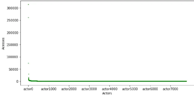
In the period being studied, there are 7778 actors. The Figure 2 shows the distribution of the number of times each actor made an access, the chart highlights two things: most actors made accesses only a few times; and a very small fraction of actors made a large number of accesses.
This distribution does not allow us to draw big conclusions because of the contrast in the values. As most actors appear only once or a few times and two actors appear 314102 and 261719 times. If the actors with many accesses are considered outliers and excluded from the study, it is possible to see the distribution curve with more detail, as presented in Figure 3.
16
It is possible to see the distribution curve more subtly but the knowledge taken is the same. Most actors made accesses very few times compared to the few that made a lot of accesses.
Since in Figure 3 the distribution of the actors that appear less than 1000 times is not very perceptive, due to the large range of values, a graphic with the distribution of only the actors that appear less than 1000 times is presented in Figure 4.
Another interesting analysis is to find how many different days each actor appears, as shown in Figure 5.
Figure 4 - Distribution of the number of times each actor, which made less than 1000 accesses, made an access
17
No actor appears more than 184 different days and, as expected, since the majority of users only makes one access, mostly appear in just one day. The curve of this distribution is much more readable since there is not so much contrast in the number of days as there is in the number of times each actor appears, which means that many of the accesses are done in the same day.
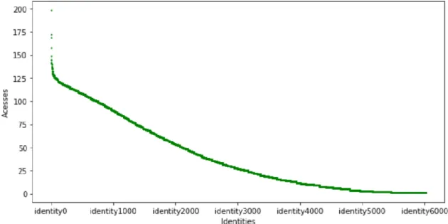
Actor_identity_id
An actor is associated with an identity id, but an identity (person) can have many accounts (actor), so the distribution of this field should be similar to the actor field.
Two actor identities appear much more than the others, -1 (means that the identity is unknown), and test user (some users are just test accounts created for monitoring reasons), which appear 326921 and 224064 times respectively. They will be left out of our distribution for better visualization of this field. Also for the same reason, to study this field we will divide it into 3 different graphics.
First, in Figure 6, we will look at the identities that made the most accesses (above 10000 times).
18
This field is empty in 13380 rows. Adding to that situations where the actor identity is not known, results in a total of 340301 times a number was accessed and there is no knowledge about the user identity id.
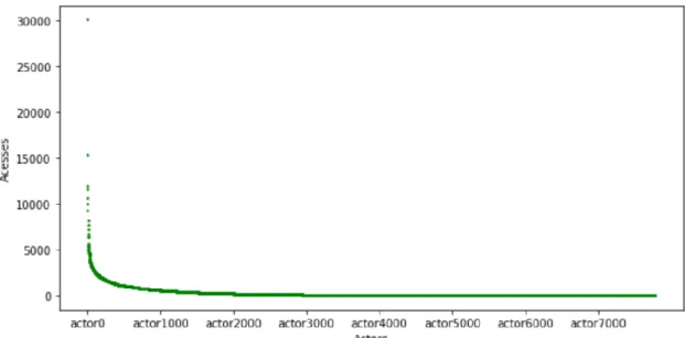
Figure 7 presents the identities that appeared between 10000 and 1000 times.
Figure 6- Distribution of the number of times each user, that made more than 10000 accesses, made an access
Ac
ce
ss
es
Identities
Figure 7- Distribution of the number of times each user, which made between 1000 and 10000 accesses, made an access
19
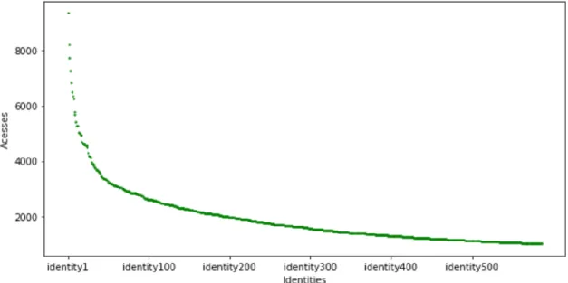
The distribution of the identities that appear more than a 1000 and less than 10000 times, is similar to the actors’ field. Few user identities were responsible for more than 1000 accesses, and very few are responsible for more than 4000.
In Figure 8 we show the distribution of the identities that appear less than 1000 times.
Most identities access telephone numbers less than 1000 times (5422 different identities), and the distribution is, as expected, very similar to the actor's distribution.
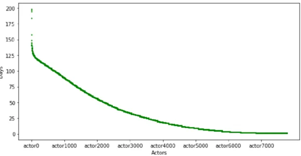
Figure 9 shows how many days each identity made accesses.
Figure 8-Distribution of the number of times each user, which made less than 1000 accesses, made an access
20
There is just one id that makes accesses every day. It will probably be a test account, but it is expected to be one of the obvious anomalies to be detected.
Action_query_phone
Action_query_phone represents the telephone number accessed by a user. It is the feature with the most variance, 641292 different telephone numbers are accessed during the period in study, therefore, once again, the distribution representation will be separated in 3 figures.
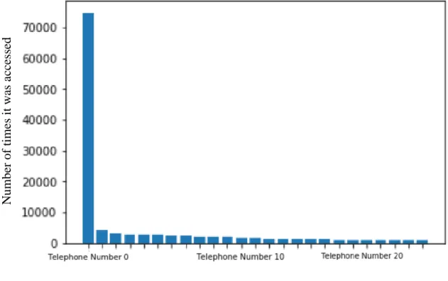
First, in Figure 10 we will be looking at the distribution of the phone numbers that are most commonly accessed (are accessed more than 1000 times).
There are 22 phone numbers that, in the period of 199 days, were accessed more than a 1000 times, the most observed number had 74766 accesses (this number is not represented graphically due to the fact that its magnitude would make the distribution much less detailed, it is a telephone number created for testing, it was considered an outlier and was excluded from the study).
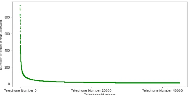
Figure 11 observes the telephone numbers that were accessed between 1000 times and 10 times.
Figure 10-Distribution of the number of times each telephone number, which was accessed more than 1000 times, was accessed
Numbe r of ti mes it wa s a cc essed Telephone Numbers
21
This distribution shows the most accentuated curve of the 3 plots since it involves a large amount of different telephone numbers and a big variance in quantities (the first has the biggest variance in quantities but very few telephone numbers, and the third has a lot of telephone numbers but a small variance in terms of quantities).
Figure 12 shows the telephone numbers accessed less than 10 times in the entire period.
As for the other fields, Figure 13 shows how many different days each telephone number is accessed, this is useful to discover what the pattern is for the number of days a
Figure 11-Distribution of the number of times each telephone number, which was accessed between 10 and 1000 times, was accessed
Figure 12-Distribution of the number of times each telephone number, which was accessed less than 1000 times, was accessed
22
telephone number is accessed, if it is normal to be constantly accessed or, for example, if the pattern is for a telephone number to be consulted just one time in the entire period.
The maximum amount of days a telephone was accessed was in 199 distinct days.
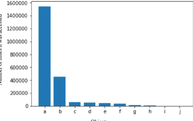
Object
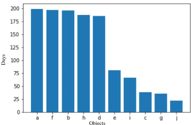
Actors access an application to read a telephone number. In Figure 14 we see which are the most common applications used. Even though this feature will not affect patterns as much as the ones presented before, it is still useful to learn its behavior.
Figure 14-Distribution of the number of times each application was used to access telephone numbers
Numbe r of ti mes it wa s ac ce ssed Objects
23
The most used applications are a and b, the first appearing in 1544429 access logs. Also interesting to see is how many different days each application is used, as shown in Figure 15.
The application that is accessed the most is a, being accessed every single day except for one.
Studying the distribution of these fields was helpful to learn which are the patterns and what is likely to be an anomaly. It was possible to see that the common behavior is for a user to do few accesses and, a user that makes several accesses may be indicative of illicit behavior.
3.2 Pre-processing
For the machine learning techniques to be effective, it was necessary to pre-process the data. After inspecting the data, it was decided which features of the original dataset are useful and should be used, which should be calculated, which should be transformed or treated, and which ones are not relevant.
Figure 15-Distribution of the number of different days each application was used to access telephone numbers
Objects
Da
y
24
As mentioned before, each log obtained from Elastic Search characterizes one access made by a user to a telephone number. Since the objective is to find anomalous behaviors, these characteristics alone will not be relevant. The relevant part is the behavior formed with the junction of accesses by user/telephone number. To obtain this, two approaches were performed.
3.2.1 User Approach
The users approach will be focused on users. The dataset created is indexed by user and has the relevant characteristics that define each user behavior. Our focus was the number of times a user made accesses, to how many telephones and in how many days. This way it is possible to detect the normal pattern of behavior and, for example, find which amounts of times or days is too much or too few, or which relations between amount of accesses and telephone numbers are more suspicious.
From the logs obtained from Elastic Search, which create the APPS-RGPD dataset, we retrieved the fields: actor_identity_id, actor, action_query_phone, ts, and object.
With these fields, a data frame was created (a type of table from the pandas3 library,
in python, very useful for machine learning) with every actor identity id. In some logs there is not identity id associated with the user. In those situations, the identity id was replaced with the actor. The field of the data frame with all the identity ids was also called Actor_identity_id. Then for each identity id, we went to the logs obtained and counted how many telephone numbers they had accessed. That field in the data frame is called Action_query_phones. Another interesting field was the number of days a user made accesses, for that the ts APPS-RGPD dataset field was used. For each access a user made, the date was checked, and it was counted in how many different days he had accessed a telephone number. The field was named Days. An obvious field to consider was the total amount of times a user made an access (field named Count in the data frame), it was simply to count how many times the id (or actor) appeared in the APPS-RGPD dataset. One more field was the number of different applications each user used. For each user we counted how many different applications that identity had in the logs object field. Finally, since this data frame was created for future applications of machine learning, the relations between these fields were also relevant. The ratio between the most significant behavior characteristics gave rise to three different fields: Ratio_Access/Tel/Days, Ratio_Access/Tel and Ratio_Access/Days. Table 2 describes each field of the dataset created for this approach.
25
Table 2-Features of the dataset created for users approach
Perspectives
To find different and specific kinds of anomalies, the algorithms were applied in different combinations of the created dataset features. This allows behaviors that could pass unnoticed when looking at all the features together. For example, a combination between the number of accesses made by the user and the number of telephone numbers the user accessed, will detect anomalies always focusing on these features, but when using
Actor_identity_id
A unique, random, anonymized user identifier. Each user is identified by his identification number, in the cases this number does not exist, the user name will be used (actor).
Counts
Total number of accesses made by the user.
Action_query_phones
Number of telephone numbers the user accessed.
Objects
Number of applications the user used to access the telephone numbers.
Days
Number of different days in which the user made an access.
Ratio_Access/Tel/Days
Ratio between the total number of accesses of the user, the number of telephone numbers accessed by the user and the number of days in which the user made accesses.
Ratio_Access/Tel
Ratio between the total number of accesses of the user and the number of telephone numbers accessed by the user.
Ratio_Access/Days
Ratio between the total number of accesses of the user and the number of days in which the user made accesses.
26
the entire dataset, if a user has these features somewhat out of the pattern but all the others are “normal” there is a higher chance that the anomaly will pass unnoticed. Table 3 describes the different perspectives analyzed.
Table 3- Different perspectives to study in users approach
AccessTel Total number of accesses made by the user and the number of telephone numbers the user accessed.
AccessDay Total number of accesses made by the user and the number of different days in which the user made an access.
TelDay The number of telephone numbers the user accessed and the number of different days in which the user made an access.
Ratios The three ratios created based on the other features.
All All the features are considered.
3.2.2 Telephones approach
The telephones approach is focused on the telephone numbers. The objective of this approach is to detect the telephone numbers that have abnormal behavior. Then select the users that have accessed those telephone numbers and verify if these have abnormal nature. Once again, from the logs obtained from Elastic Search, which create the APPS-RGPD dataset, we retrieved the same fields: actor_identity_id, actor, action_query_phone, ts, and object. The difference came in the way these fields were used to create the new dataset.
A new dataframe was created, this one with every telephone number. Then it was counted, from the logs of accesses, how many different users had accessed each telephone number. This field was called Actors. The field Days was created again, but this time, for each time a telephone number was accessed, the date was checked and it was counted how many different days each telephone number was accessed. Another field that was also created was Count, the total number of times a telephone number was accessed. It was as simple as counting the number of times a telephone number appeared in the access logs. The field Objects in the dataframe means the number of different applications each telephone number was accessed by. For each telephone number, it was counted how many different applications had been used by users in the logs object field. Finally, just like in the users approach, the relations between these fields were also relevant. The ratio
27
between the most significant behavior characteristics gave rise to the three different fields: Ratio_Access/Actor/Days, Ratio_Access/Actor and Ratio_Access/Days. Table 4 describes each field of the dataset created for this approach.
Table 4--Features of the dataset created for telephones approach
Action_query_phone
The telephone number.
Count
Number of times that telephone number was accessed.
Actors
Number of users that accessed that telephone number.
Object
Number of applications users used to access that telephone number.
Days
Number of different days in which the telephone number was accessed.
Ratio_Access/Actor/Day
Ratio between the total number of times the telephone number was accessed, the number of users that accessed the telephone number and the number of days in which the telephone number was accessed.
Ratio_Access/Actor
Ratio between the total number of accesses of the user and the number of telephone numbers accessed by the user.
Ratio_Access/Days
Ratio between the total number of times the telephone number was accessed and the number of days in which the telephone number was accessed.
28 Perspectives
Just like for the users approach, we need to look at different perspectives of the dataset to detect the different types of anomalies. These are presented in Table 5.
Table 5- Different perspectives to study in telephones approach
AccessActor
Total number of times a telephone number was accessed and the number of users that accessed it.
AccessDay
Total number of times a telephone number was accessed and the number of different days in which it was accessed.
DayActor
The number of different days in which the telephone number was accessed and the number of users that accessed it.
Ratios The three ratios created based on the other features.
All All the features are considered.
3.2.3 Normalization
. Like in most machine learning situations, since we are dealing with features with very different intervals, the data needs to be normalized. Since, this data has “noise” (the data contains anomalies that are not supposed to be considered in the normal interval of each feature), instead of using the maximum and minimum number of a feature, we decided to use the 3rd quartile (75th quantile) and 1st quartile (25th quantile), respectively, therefore instead of the median we scale the data according to the quantile range. This means that Robust Scaler was the normalization method chosen.
3.3 Anomalies
Both datasets will be explored in various ways, to detect specific types of anomalies with the different algorithms. The types of anomalies considered are described in Table 6.
29
Table 6- Labels created to classify anomalies
1st type of anomaly Many accesses to many telephone numbers, in many days
2nd type of anomaly Many accesses to some telephone numbers, in many days
3rd type of anomaly Many accesses to one or few telephone numbers, in many days
4th type of anomaly Many accesses to many telephone numbers, in one or few days
5th type of anomaly Many accesses to some telephone numbers, in one or few days
6th type of anomaly Many accesses to one or a few telephone numbers, in one or few days
7th type of anomaly Many accesses to a telephone number, just one day
8th type of anomaly Some accesses to a telephone number, just one day
9th type of anomaly Some accesses to one or a few telephone numbers, in one or few days
10th type of anomaly Extreme cases (obvious anomalies)
All of these types could be relevant depending on the specific situation looked for. The 3rd, 4th and 7th type of anomaly are the ones that represent the most pertinent situations looked for.The 3rd type of anomaly could be a case of stalking or tracking. Someone is following
the activity of a certain telephone for a long period. The 4th type represents a massive
extraction of information of various telephone numbers in a short period. This could mean that someone is performing a fast search to raise clients for another telecommunications company. The 7th type, a massive extraction of information of a telephone number in a
short period. This could mean, for example, someone is searching for some specific information about a telephone number. All these situations are examples of very relevant cases this project intends to detect. Even though the other ones are not as much of a priority, they could also represent relevant cases. The 8th type of anomaly, for example, could be a situation of someone searching for a telephone number because a friend from the outside of the company asked for. The same goes for the 9th anomaly type, but in this
30
case, instead of one, the person would be searching in two or three telephone numbers. The 10th type is very likely a test account due to its behavior numbers being so high. Succinctly, all the types could represent a relevant situation of illicit accesses to clients telephone numbers information, but a few types have priority, due to its specificity towards what we are looking for.
3.4 Algorithms
When it came to choosing the algorithms that were going to be used we tried to diversify. Both clustering and anomaly detection algorithms were taken into consideration. Anomaly detection algorithms to serve their purpose and clustering algorithms to divide the data in a way that it is possible to interpret the separation of the anomalies from the users that follow the pattern, meaning that bigger clusters represent identities that follow the pattern, and very small and more distant clusters represent identities having an “abnormal” behavior. In the case of DBSCAN, not only it returns clusters but also the identities that do not fit any cluster. These identities will also be interpreted as anomalies. K-means and DBSCAN were considered because they are two different general purpose clustering methods, affinity propagation was used because it has the ability to determine the number of clusters without specific parameters.
3.4.1 K-means
One of the algorithms used was K-means4. Since it is the most known and tested
clustering algorithm it was relevant to take it into account. Since in the beginning the important is to start understanding the data and try different things, we started by it. Even though it is the most known and very simple clustering algorithm it can obtain very good results as seen in “A survey of network anomaly detection techniques” [5].
The most important parameter in this algorithm is the number of clusters chosen. This was the parameter that had to be optimized.
Parameters used:
N_clusters: The number of clusters to form (To be decided in the parameterization
step);
Init: Method for initialization (‘means++’, selects initial cluster centers for k-means clustering in a smart way to speed up convergence);