* Corresponding author:
E-mail: [email protected]
Received: September 26, 2015
Approved: June 22, 2016
How to cite: Demattê JAM, Alves MR, Terra FS, Bosquilia RWD, Fongaro CT, Barros PPS. Is It Possible to Classify Topsoil Texture Using a Sensor Located 800 km Away from the Surface? Rev Bras Cienc Solo. 2016;40:e0150335.
Copyright: This is an open-access article distributed under the terms of the Creative Commons Attribution License, which permits unrestricted use, distribution, and reproduction in any medium, provided that the original author and source are credited.
Is It Possible to Classify Topsoil
Texture Using a Sensor Located
800 km Away from the Surface?
José Alexandre Melo Demattê(1)*
, Marcelo Rodrigo Alves(2)
, Fabricio da Silva Terra(3) , Raoni Wainer Duarte Bosquilia(4)
, Caio Troula Fongaro(1)
and Pedro Paulo da Silva Barros(5)
(1)
Universidade de São Paulo, Escola Superior de Agricultura “Luiz de Queiroz”, Departamento de Ciência do Solo, Piracicaba, São Paulo, Brasil.
(2)
Universidade do Oeste Paulista, Faculdade de Agronomia, Presidente Prudente, São Paulo, Brasil. (3)
Universidade Federal de Pelotas, Centro de Desenvolvimento Tecnológico/Engenharia Hídrica, Pelotas, Rio Grande do Sul, Brasil.
(4)
Universidade Tecnológica Federal do Paraná, Dois Vizinhos, Paraná, Brasil. (5)
Universidade de São Paulo, Escola Superior de Agricultura “Luiz de Queiroz”, Departamento de Biossistemas, Piracicaba, São Paulo, Brasil.
ABSTRACT: It is often difficult for pedologists to “see” topsoils indicating differences in
properties such as soil particle size. Satellite images are important for obtaining quick information for large areas. However, mapping extensive areas of bare soil using a single image is difficult since most areas are usually covered by vegetation. Thus, the aim of this study was to develop a strategy to determine bare soil areas by fusing multi-temporal satellite images and classifying them according to soil textures. Three different areas located in two states in Brazil, with a total of 65,000 ha, were evaluated. Landsat images of a specific dry month (September) over five consecutive years were collected, processed, and subjected to atmospheric correction (values in surface reflectance). Non-vegetated areas were discriminated from vegetated ones using the Linear Spectral Mixture Model (LSMM) and Normalized Difference Vegetation Index (NDVI). Thus, we were able to fuse images with only bare soil. Field samples were taken from bare soil pixel areas. Pixels of soils with different textures (soil texture classifications) were used for supervised classification in which all areas with exposed soil were classified. Single images reached an average of 36 % bare soil, where the mapper could only “see” these points. After using the proposed methodology, we reached a maximum of 85 % in bare areas; therefore, a pedologist would have proper conditions for generating a continuous map of spatial variations in soil properties. In addition, we mapped soil textural classes with accuracy up to 86.7 % for clayey soils. Overall accuracy was 63.8 %. The method was tested in an unknown area to validate the accuracy of our classification method. Our strategy allowed us to discriminate and categorize different soil textures in the field with 90 % accuracy using images. This method can assist several professionals in soil science, from pedologists to mappers of soil properties, in soil management activities.
Keywords: bare soils, satellite images, spectral sensing, multi-temporal images, digital soil mapping, soil remote sensing.
INTRODUCTION
Orbital remote sensing in a country of continental dimensions, such as Brazil, is an indispensable tool for understanding and monitoring natural resources (Lima et al., 2001). Soils play a very important role in plant development and global food production, but soils have typically been used without proper knowledge, characterization, and studies. Improper land use results in soil degradation, low crop yield, and high costs from unsustainable production.
One of the most important soil properties is texture, due to its relationship with other properties, such as structure, porosity, permeability, fertility, chemistry, and moisture content (Brady and Weil, 2007). Soil texture is obtained from soil particle size distribution, which is mainly analyzed and mapped using traditional approaches in which pedologists make boreholes in the field or collect samples from soil profiles and analyze their findings in a laboratory. This procedure is costly and time-consuming. However, areas with high intensity agriculture need this information. Thus, there is the need for a more effective method of mapping soil texture. Remote sensing is an important tool for soil surveying. In particular, many studies have found that texture can be quantified by spectral reflectance under laboratory conditions (Nanni and Demattê, 2006). Nanni et al. (2012) have also observed the importance of orbital images for clay estimates. These studies have shown that it is possible to determine soil particle distribution (clay, silt, and sand percentages) by spectral data. Identification of bare soils by satellite imaging is not new (e.g. Demattê et al., 2009; Ghaemi et al., 2013; and Masoud, 2014), but continuous information on bare soils in an area is still an important difficulty for soil scientists, especially pedologists.
Spectral data from orbital levels usually show vegetated areas where it is not possible to detect soil information. Therefore, how can a pedologist map an area if only certain spots of bare soil are shown in a single image? This problem has been observed in field studies; if we had one image with all the information from bare soil, the survey would certainly be easier. Methodologies that are well-performed have been restricted to spots of bare soil. Brazil and African countries, in tropical regions, have extensive areas of agriculture, and information on soil texture from orbital data can assist soil surveying and mapping.
In this context, the aim of the present study was to develop a strategy to identify continuous areas of bare soil by fusing multi-temporal orbital images of the same location and by mapping the topsoils according to soil textural classification. The hypothesis of our research is that changes in soil texture affect spectral data, which can be detected and mapped by satellite images. In addition, the strategy we propose is based on field observation of conventional agricultural areas with bare soils in different periods of the year, where the fusion of images from different years can provide a complete “picture” of bare soil.
MATERIALS AND METHODS
Description of study sites
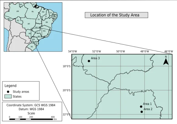
Three sites were chosen: two in the state of São Paulo and one in the state of Goiás (Figure 1). The study sites covered a total of 30,000 ha in São Paulo (15,000 ha each) and 35,000 ha in Goiás. All sites are at altitudes ranging from 450 to 900 m; the climate is temperate with dry winters (Aw - Köppen classification system), with average annual rainfall ranging from 1,000 to 1,800 mm and average temperature of 20 °C. The lithology is mainly represented by the Serra Geral, Botucatu, and Pirambóia (São Bento Group) Formations, and Serra de Santana covers (Taubaté Group). The rocks from the Serra Geral
Formation are volcanic of basaltic origin; the rocks from the Botucatu Formation are eolic sandstones; and the rocks from the Pirambóia Formation are composed of sandstones from river deposits and floodplains (Bistrichi et al., 1981). The soils at the sites are mainly classified as Arenosols and Ferralsols (WRB, 2014) and Neossolos Quartzarênicos and
Database
This study was divided into three steps: (1) to determine a methodology for measuring exposed continuous soil areas with no vegetation in Area 1 from the state of São Paulo; (2) to perform a theoretical validation in Area 2 from the state of São Paulo; and (3) to perform a practical validation in an unknown area from a different region (Area 3 in the state of Goiás) to check the potential of the method. First, we needed to understand the textural condition of the target areas at the terrestrial level before analyzing it at the satellite level. For that purpose, topsoil samples were obtained along toposequences (transect method). We collected 300 soil samples at a depth of 0.00-0.20 m from 20 toposequences (Figure 2) and their georeferenced images. After that, we analyzed soil particle distribution to determine the contents of coarse and fine sands, silt, and clay in the soil samples (Camargo et al., 1987). Clay contents were grouped into five textural classes, according to Santos et al. (2013): sandy (<150 g kg-1 of
clay), sandy loamy (150 to 250 g kg-1 of clay), clayey loamy (250 to 350 g kg-1 of clay), clayey
(350 to 600 g kg-1 of clay), and heavy clayey (>600 g kg-1 of clay). Soils in these areas were
mostly classified as Arenosols and Ferralsols (WRB, 2014). Then, the 300 sampling points were positioned in pixels corresponding to bare soils.
Satellite data acquisition and processing – fusion preparation
Five TM/Landsat-5 images were used in order to obtain consecutive years in the same season. September was chosen since the soil is usually dry in this month. In large agricultural areas cultivated with sugarcane, traditional tillage resulting in bare soils was practiced in different areas from one year to the next. This is a five-year cycle, which means that an area tilled in a given year will only be tilled again five years later. Within a five-year period, all parts of a given area should have bare soil. Thus, our strategy was to collect images from different years to detect spots of bare soils and construct a map like a “puzzle”, where each piece is related to bare soil from a specific year.
The images were georeferenced using ground control points obtained from GPS, and the nearest neighbor was used as an interpolation method (RSI, 2006) to maintain the pixel
Figure 1. Location of the study area. Area 1: Calibration; Area 2: Validation stage 1; Area 3: Validation in practice (Field).
Area 2 Area 3
Area 1
46°0'W 48°0'W
50°0'W 52°0'W
54°0'W
18°0'S
20°0'S
22°0'S AM PA
MT BA
MG PI
MS
RS GO
MA
TO
SP RO
PR AC
AP
SC RR
0 100 200 400
Scale
Legend
Study areas States
Coordinate System: GCS WGS 1984 Datum: WGS 1984
CE
Location of the Study Area
Km
value similar to its original value. After that, atmospheric correction was performed by the 6S program (Second Simulation of the Satellite Signal in the Solar Spectrum) to convert digital numbers into surface reflectance values (Vermote et al., 1997). The 6S program allows geometric configuration of specific satellites, such as Landsat 5, to be selected.
For each satellite image, the Linear Spectral Mixture Model (LSMM) was used to discriminate vegetated areas from images of bare soil (Demattê et al., 2009), reducing pixel mixture and quantifying proportions of pure elements that constitute the pixel mixture (Shimabukuro and Smith, 1991). After using the LSMM, the following image-processing procedures were performed to indicate the true nature of the pixel: A) determination of NDVI images (Equation 1), B) evaluation of the pixel position at the soil line, C) display of the false-color band combination of bands 5 (1.55 to 1.75 µm), 4 (0.76 to 0.90 µm), and 3 (0.63 to 0.69 µm) as red, green, and blue, respectively, D) display of the true-color band combination of bands 3, 2 (0.520 to 0.600 µm), and 1 (0.450 to 520 µm) as red, green, Figure 2. Distribution scheme of sampling points in Area 1 (calibration phase) as well as in Area 2 (validation phase), and determination of eight sub-areas for the validation phase.
Work area 1 Work area 2
Work area 2 divided into sub-areas
1
7 6
8 5
2 4
3
Distribution of the sampling points for validation of supervised classification Distribution of the sampling points
and blue, respectively, and E) determination of the pixel spectral manifestation (spectral shape), as described by Demattê et al. (2009). Thus, only when all these procedures simultaneously indicated a pixel as bare soil was the pixel used for subsequent analysis. Pixels were rejected if at least one of these procedures, such as NDVI, indicated any possibility of contribution from vegetation in their spectral reflectance (Demattê et al., 2009). Only pixels that met all the requirements were used to establish the library for a certain soil class. With the information on bare soil positions for each image, a mask was made excluding all vegetated areas using the following equation:
NDVI = IV – VIS
IV + VIS Eq. 1
where IV is the spectral pixel response in the near infrared (TM 4) and VIS is the spectral response in the visible pixel (TM 3). The images corresponding to different seasons were individually classified using the Gaussian Maximum Likelihood algorithm (supervised classification), where bands 1, 2, 3, 4, 5, and 7 were used in the classification. The vector file containing the 300 sampling points with information related to soil textural classes was overlaid with the surface reflectance images. The reflectance of pixels at each sampling point was obtained, and five regions of interest (ROIs) were designated, corresponding to each soil texture class. All pixels that were not identified by supervised classification as belonging to any specific textural class were defined as “NoData” and were reclassified to zero value. The images displayed only pixels related to classes of interest. After that, a fusion of all five classified images with their respective portions of bare soils was obtained by overlapping them. We suggested the name of fused image (FI) for this final product. A mosaic with five supervised classification images (SCI) was designed to show the largest possible area covered by the supervised classification in a single image. Thus, a mosaic of exposed soils was generated and soil texture was classified.
In the validation stage (Step 3), data from Area 1 were tested in Area 2. Area 2 was subdivided into smaller continuous areas (Figure 2). Both SCI and the fused image were cut off based on these sub-areas and were subjected to the “Zonal Geometry” routine of the ArcGis 9.2 program to calculate the percentage of bare soil obtained by supervised classification. We positioned 204 other sampling points over this unknown area. These soil samples were collected, analyzed (as described earlier), and classified according to textural classes. We considered these data points as “reference data” and compared them with pixels obtained from the fused image. From this comparison, a contingency table (error or confusion matrix) was obtained. In addition, we performed correlation between the test results and determined the percentages of correct answers for each class, as well as overall accuracy and the Kappa index (Cohen, 1960) (Equation 2).
^
K = θ1 – θ2 1 – θ2
Eq. 2
θ1 =
1
N Ʃ
n
i = 1mn Eq. 3
θ2 =
1 N2 Ʃ
n k = 1 (Ʃ
n
i = 1 mik×Ʃ n
j = 1 mkj) Eq. 4
where K^ is the Kappa coefficient, n is the number of columns and rows of the matrix confusion, mij is the element (i,j) of the matrix confusion, and N is the total number of observations. Finally, an in situ field validation was performed. For this validation,
RESULTS AND DISCUSSION
Fused image of bare soils
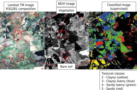
The sand class showed the largest number of observations (83) and the highest coefficient of variation (Table 1). The contents of organic matter (OM) analyzed in the sites had low variation, from 0.5 to 0.7 %. Chemical analysis also indicated very low fertility and cation exchange capacity (CEC) (Table 1). However, particle size distribution was the soil property that most influenced the spectra. Considering all textures within an area of 15,000 ha, we found high and similar numbers of samples. The only exception was for heavy clayey. In fact, heavy clayey is a very specific class and does not occur in this site. The SCI obtained from Landsat images and classified according to the four soil texture classes covered only areas of bare soil, which was evident when we simultaneously observed satellite images, NDVI images, and the SCI (Figure 3). The satellite image was visualized with the following composition: R (band 3), G (band 2), and B (band 1), whereas the NDVI image represented exposed soil by a dark color and vegetation by a light color. The fact that SCI involved only areas of exposed soil is very important because this exposure is necessary to perform analysis of soil texture by satellite imaging.
Table 1. Clay contents of 300 samples in phase 1 (area 1)
Class Criterion n(1)
Minimum Maximum Average Amplitude SE(2)
CV(3) g kg-1
%
Clayey >600 02 613.0 745.0 679.0 132.0 93.3 13.7
Very clayey 351-600 71 353.0 587.0 427.8 234.0 58.8 13.7
Clayey loamy 251-350 64 251.0 350.0 295.3 99.0 28.4 9.6
Sandy loamy 151-250 80 151.0 250.0 201.2 99.0 31.2 15.5
Sandy ≤150 83 72.0 150.0 113.8 78.0 19.4 17.1
(1)
n: number of samples; (2)
SE: standard error; (3) CV: coefficient of variation.
Figure 3. Sequence of observations from Landsat image, NDVI image, and supervised classification image (Demattê et al., 2009).
NDVI image
Textural classes 2 - Clayey (yellow) 3 - Clayey loamy (blue) 4 - Sandy loamy (green) 5 - Sandy (red)
Landsat TM image R3G2B1 composition
Classified image (supervised)
When we analyzed images for each year, areas that were classified as N.Class (Not
classified) were larger than the useful area to which we applied the supervised classification (Table 2, Figure 4). N.Class areas were not classified (in the respective
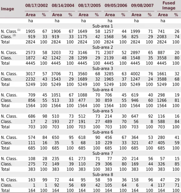
season) because they had vegetation cover. We determined that, on average, 63 % of the total area of each sub-area showed N.Class values compared with only 37 % of the total area with bare soils. When we used a single image, we had an average of 36.2 % considered as bare soils. On the other hand, using the fused image, we obtained an average of 75.2 %, a minimum of 59 %, and a maximum of 85 % considered as bare soil. The study sites were cultivated; therefore, they have some type of plant cover through most of the year, hindering analyses by satellite imaging. Such information highlights the problem of working with images from only one season. For example, in the case of an image dated from Aug. 17, 2003, sub-area 7 showed a percentage of useful area of 72 %, while sub-area 8 showed a percentage of only 1 % (Table 2). Thus, it is impossible to use images of Area 3 for soils using this date (Figure 5). On the other hand, the importance of evaluating images in different years can be observed in sub-area 8. From 2002 to 2007 (with exception of 2003), the bare soil rate was 1, 56, 42, 63, and 3 %, respectively. In practice, a pedologist could obtain a maximum area with 63 % bare soil analyzing only one image. When we used the proposed method, we obtained 75 % bare soil (Table 2, Figure 5).
Table 2. Quantitative statistics of exposed soil areas in each study sub-area and in different years
Image 08/17/2002 08/14/2004 08/17/2005 09/05/2006 09/08/2007
Fused Image
Area % Area % Area % Area % Area % Area %
ha ha ha ha ha ha
Sub-area 1 N. Class.(1)
1905 67 1906 67 1649 58 1257 44 1999 71 741 26
Class. (2)
919 33 919 33 1175 42 1568 56 825 29 2083 74
Total 2824 100 2824 100 2824 100 2824 100 2824 100 2824 100
Sub-area 2
N. Class. 2573 58 3203 72 3146 71 2307 52 2897 65 887 20
Class. 1872 42 1242 28 1299 29 2139 48 1548 35 3558 80
Total 4445 100 4445 100 4445 100 4445 100 4445 100 4445 100
Sub-area 3
N. Class. 3017 57 3706 71 3560 68 3285 63 4002 76 1661 32
Class. 2232 43 1543 29 1689 32 1965 37 1247 24 3588 68
Total 5249 100 5249 100 5249 100 5249 100 5249 100 5249 100
Sub-area 4
N. Class. 709 45 1051 67 1088 70 706 45 619 40 298 19
Class. 856 55 513 33 477 30 859 55 946 60 1266 81
Total 1564 100 1564 100 1564 100 1564 100 1564 100 1564 100
Sub-area 5
N. Class. 686 98 510 73 512 73 214 30 647 92 116 16
Class. 17 2 193 27 191 27 489 70 56 8 588 84
Total 703 100 703 100 703 100 703 100 703 100 703 100
Sub-area 6
N. Class. 574 84 650 95 618 90 456 67 364 53 280 41
Class. 111 16 35 5 68 10 229 33 321 47 405 59
Total 685 100 685 100 685 100 685 100 685 100 685 100
Sub-area 7
N. Class. 108 28 235 61 273 71 77 20 214 56 57 15
Class. 275 72 149 39 110 29 306 80 169 44 326 85
Total 383 100 383 100 383 100 383 100 383 100 383 100
Sub-area 8
N. Class. 163 99 72 44 95 58 59 36 158 96 47 29
Class. 1 1 92 56 69 42 105 64 6 4 117 71
Total 164 100 164 100 164 100 164 100 164 100 164 100
When data on fused images were analyzed, we observed an increase in useful area for all sub-areas (Table 2). The FI for sub-area 6 showed the lowest percentage of useful area (59 %). However, when comparing this value with the best result achieved in a single image (dated from Sept. 08, 2007 with 47 % of useful area), there was a gain of 26 %. The FI of sub-area 7 showed the largest percentage of useful area (85 %) (Figure 5), followed by sub-areas 5, 4, and 2 (84, 81, and 80 %, respectively) (Figures 4 and 5). Comparing these values with the best results in a single image, it appears that for sub-areas 7, 5, 4, and 2, there were increases of 6, 20, 34, and 66 %, respectively. These increases were associated with the size of the total area, that is, the larger the total area, the greater the increase the FI provides. The importance of the FI was evident when we analyzed the average useful area of bare soils, which increased from 36 to 75 %, representing a gain of more than 100 % with the use of the mosaic. Thus, there was an increase in the useful area compared with data related to single images.
Theoretical validation stage (soil surface texture classification by satellite data)
To validate our results and determine the ability to predict topsoil textural class, the clay content of 204 sampling points was analyzed by the conventional method (reference data) and compared to values obtained by supervised classification (estimated values). These points were distributed over four textural classes (Table 3) and their clay content ranged from 48 to 554 g kg-1.
The confusion matrix represented the relationship between texture reference data (soil analysis) and values estimated by supervised classification (Table 4). Classification accuracy indicated that the clayey class attained the highest level of success (86.7 %), followed by the clayey loamy (60.6 %), sandy loamy (56.6 %) and sandy (52.2 %) classes. These Figure 4. Coverage of the supervised classification image in each image by sub-areas (1, 2, 3, and 4) and mosaic of all the images. Yellow color is for clayey soils, blue for clayey loamy soils, green for sandy loamy soils, and red for sandy soils.
Image 2002 Image 2004 Image 2005 Image 2006 Image 2007 Mosaic
Sub area 4
Sub area 3
Sub area 2
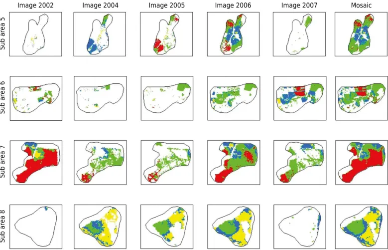
Figure 5. Coverage of the supervised classification image in each image by sub-areas (5, 6, 7, and 8) and mosaic of all the images. Yellow color is for clayey soils, blue for clayey loamy soils, green for sandy loamy soils, and red for sandy soils.
Image 2002 Image 2004 Image 2005 Image 2006 Image 2007 Mosaic
Sub area 8
Sub area 7
Sub area 6
Sub area 5
Table 4. Confusion matrix generated from the similarity between values determined by the
conventional method and by the supervised classification method (estimated values)
Texture classes
Supervised classification (% agreement with image)
Clayey Clayey loamy
Sandy
loamy Sandy
Clayey 86.7 11.1 2.2 0.0
Clayey Loamy 33.3 60.6 6.1 0.0
Sandy Loamy 11.3 28.3 56.6 3.8
Sandy 6.5 10.9 30.4 52.2
Overall accuracy (%) 63.8
Kappa index 0.52
Table 3. Descriptive analysis of database used to validate the method of determining the soil
texture class, at the surface, by supervised classification (204 samples in Area 2)
Class Criterion n(1)
Minimum Maximum Average Amplitude SE(2)
CV(3) g kg-1
%
Clayey >600 - - -
-Very clayey 351-600 53 353.0 554.0 418.0 201.0 53.3 12.7
Clayey loamy 251-350 39 259.0 350.0 308.5 91.0 25.5 8.3
Sandy loamy 151-250 63 151.0 249.0 201.9 98.0 26.5 13.2
Sandy ≤150 49 48.0 148.0 114.1 100.0 26.3 23.1
(1)
n: number of samples; (2)
values were higher than those found by Demattê et al. (2005) for a similar area. Some confusion was observed, such as 33.3 % of the clayey class was mixed with the clayey loamy class. The sandy loamy class with 56.6 % agreement had 28.3 % misclassified as the clayey loamy class. The confusion in supervised classification was mostly related to the correct texture class.
Topsoils of clayey texture were discriminated from soils of the sandy class in 100 % of the classification, that is, none of the clayey soils were classified as sandy texture. Okin et al. (2001) had considerable success in discriminating clayey from sandy soils, with approximately 90 % accuracy. However, the authors conducted the experiment with the high spectral resolution Airborne Visible and Infrared Imaging Spectrometer (AVIRIS) using the MESMA method. This sensor has 224 spectral bands and is considerably more powerful than the Landsat, which explains their better results. Coleman et al. (1993) started with 0.4 R² for clay using Landsat. Nanni and Demattê (2006) reached 67 % accuracy for the clayey class when evaluated an area with full exposure of non-vegetated areas (bare soils). Demattê et al. (2009) reached 90 % accuracy evaluating 224 pixels in a 300,000 ha area, but in this case, it was all done in a single image. The fact is that the present methodology reached a classification accuracy ranging from 60 to 86 % for some soil texture classes using multi-spectral Landsat images (only six bands) and fused images from several seasons. Moreover, the methodology used in this study generated continuous areas with bare soil that can provide more sustainable information to pedologists. Still, we have to keep in mind that the soil sample was collected in a single spot that corresponds to a 0.20 m2 (the
borehole) and the pixel of the image covers 30 m2. Moreover, the sensor is located
at a distance of 800 km from the target.
The overall accuracy (63.8 %) (Table 4) was lower than the minimum acceptable value (85 %) according to Guptill and Morrison (1995). Considering the classes individually, we observed that clayey texture was the only class whose value was higher than the minimum acceptable value, and the Kappa index obtained (0.52) was considered appropriate by the Landis and Koch (1977) classification, suggesting that the method can be used to indicate soil texture on the surface.
In situ evaluation
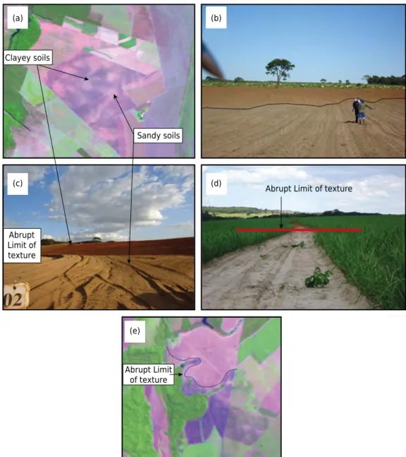
In areas located in the state of Goiás, we created a fused image of exposed soils, as mentioned in the methodology. We used a 543 RGB color composition based on the image and an unsupervised classification. We then went to the field using GPS, and with the image in a Palmtop, we went to spots already expecting to see the soil texture. This in situ approach was illustrated in figure 6. For each validation spot,
we went to the field and determined its texture (at 200 points). We determined that the different spectral information detected in the image enabled differentiation of soil texture. The soils of these areas are mostly Arenosols and Ferralsols, which have no texture variation with depth. Thus, determining surface texture represents most of the soil. Since these are very large areas, determining soil texture as “continuous” would be highly cost-effective. The OM content did not influence the results, because it was similar in all areas, ranging from 0.3 to 0.5 %. In many situations, we observed light colors in the 543 RGB image and expected to “see” sandy soils. In fact, upon reaching the spot, we made the borehole, and a sandy texture was detected. We observed that 90 % of the soil samples in situ were in the same texture classification as indicated
by the image. The image also indicated spatial variation (Figure 6). This information can assist farmers in making a texture map to assist agriculture practices, such as the use of herbicides.
The use of hyperspectral images is clearly the best choice because of the great number of bands. However, these data are still under development, and they are difficult to use and somewhat costly. AVIRIS, with its 224 bands, is a private sensor and is not available to users. Hyperion has low quality (high noise information) and does not have high temporal information. Thus, we need an easy and inexpensive method to assist users. In this context, Landsat has high temporal information and free access, achieving fairly good results, as presented in this study.
CONCLUSIONS
Using the fused image (FI) methodology of multi-temporal images of the same region, the bare soil area was increased from 36 to 75 %, representing a gain of more than 100 %. There is wide variation in the amount of bare soil in satellite images at the same site in different seasons, ranging from 1 to 65 %. This range indicates the importance of evaluating images in different years (time series). In our methodology, the use of images from different periods enabled us to map more than 75 % of the total area studied, an increase of up to 60 % when compared with the use of a single image.
Figure 6. Illustration of field work: (a) Landsat image indicating areas with bare soils, sandy and
clayey; (b) soil variability and sampling in the field; (c) Soil variability in an area with bare soil; (d) Soil
variability in an area with vegetation cover; and (e) Landsat image indicating variations in soil texture. Sandy soils
Clayey soils
Abrupt Limit of texture
Abrupt Limit of texture
Abrupt Limit of texture
(a) (b)
(c) (d)
The validation study indicated that clayey and clayey loamy texture classes had the best performance, with 86.7 and 60.6 % success, respectively. Discrimination of clayey from sandy soil was 100 % successful.
The in situ field approach and validation indicated 90 % agreement of surface soil texture
compared with the pixel information from the fused image in an unknown area.
The method achieved promising results considering that we used a multispectral sensor 800 km distant from the target and a 30 m2 pixel. This can assist users by means of an easy and inexpensive method since Landsat information is free on the Internet.
REFERENCES
Bistrichi CA, Carneiro CDR, Dantas ASL, Ponçano WL, Campanha GAC, Nagata N, Almeida MA, Stein DP, Melo MS, Cremonini OA. Mapa Geológico do Estado de São Paulo. 1981. [acesso: 10 Ago 2009]. Disponível em: http://geobank.sa.cprm.gov.br.
Brady NC, Weil RR. The nature and properties of soil. London: Pearson Prentice Hall; 2007. Camargo MN, Klant E, Kauffman JH. Classificação de solos usada em levantamentos pedológicos no Brasil. Bol Inf Soc Bras Cienc Solo. 1987;12:11-3.
Cohen JA. Coefficient of agreement for nominal scales. Educ Psychol Measur. 1960;20:37-46. doi:10.1177/001316446002000104
Coleman TL, Agbu PA, Montgomery OL. Spectral differentiation of surface soils and soil properties: is it possible from space platforms? Soil Sci. 1993;155:283-93. doi:10.1097/00010694-199304000-00007
Demattê JAM, Galdos MV, Guimarães RV, Gení AM, Nanni, MR, Zulu J. Quantification of tropical soil attributes from ETM+/Landsat-7. Int J Rem Sensing. 2007;24:257-75. doi:10.1080/01431160601121469
Demattê JAM, Huete A, Guimarães L, Nanni MR, Alves MC, Fiorio PR. Methodology for bare soil detection and discrimination by Landsat-TM image. Open Rem Sensing J. 2009;2:24-35. doi:10.2174/1875413900902010024
Demattê JAM, Moreti D, Vasconcelos ACF, Genú AM. Uso de imagens de satélite na
discriminação de solos desenvolvidos de basalto e arenito na região de Paraguaçu Paulista. Pesq Agropec Bras. 2005;40:697-706. doi:10.1590/S0100-204X2005000700011
Ghaemi M, Astaraei AR, Sanaeinejad SH, Zare H. Using satellite data for soil cation exchange capacity studies. Int Agrophys. 2013;27:409-17. doi:10.2478/intag-2013-0011
Guptill SC, Morrison JL. Elements of spatial data quality. New York: Elsevier; 1995. IUSS Working Group - WRB. World Reference Base for Soil Resources. International soil classification system for naming soils and creating legends for soil maps. Rome: FAO; 2014. (World Soil Resources Reports, 106).
Landis JR, Koch GG. The measurement of observer agreement for categorical data. Biometrics, 1977;33:159-74. doi:10.2307/2529310
Lima ZMC, Ribeiro MR, Lima ATO. Utilization of TM/LANDSAT-5 images as a tool in soil survey. Rev Bras Eng Agríc Amb. 2001;5:425-30. doi:10.1590/S1415-43662001000300010
Masoud AA. Predicting salt abundance in slightly saline soils from Landsat ETM+ imagery using Spectral Mixture Analysis and soil spectrometry. Geoderma. 2014;217-218:45-56. doi:10.1016/j.geoderma.2013.10.027
Nanni MR, Demattê JAM, Chicati ML, Fiorio PR, Cezar E, Oliveira RB. Soil surface spectral data from Landsat imagery for soil class discrimination. Acta Sci Agron. 2012;34:103-12. doi:10.4025/actasciagron.v34i1.12204
Okin GS, Murray B, Schlesinger WH. Degradation of sandy arid shrubland environments: observations, process modelling, and management implications. J Arid Environ. 2001;47:123-44. doi:10.1006/jare.2000.0711
Research Systems Inc. - RSI. The Environment for Visualizing Images – ENVI. Boulder: 2006. Santos HG, Jacomine PKT, Anjos LHC, Oliveira VA, Oliveira JB, Coelho MR, Lumbreras JF, Cunha TJF. Sistema brasileiro de classificação de solos. 3a ed. Rio de Janeiro: Embrapa Solos; 2013. Shimabukuro YE, Smith JA. The least-squares mixing models to generate fraction images derived from remote sensing multispectral data. IEEE Trans Geosci Rem Sensing. 1991;29:16-20. doi:10.1109/36.103288