DOCUMENTOS DE TRABALHO
WORKING PAPERS
ECONOMIA
ECONOMICS
Nº 15/2007
ASYMMETRIC COLLUSION AND MERGER POLICY
Mattias Ganslandt
Research Institute of Industrial Economics (IFN)
Lars Persson
Research Institute of Industrial Economics (IFN) and CEPR
Hélder Vasconcelos
Asymmetric Collusion and Merger Policy
Mattias Ganslandt
Research Institute of Industrial Economics (IFN)
Lars Persson
Research Institute of Industrial Economics (IFN) and CEPR
Helder Vasconcelos
Universidade Católica Portuguesa and CEPR
September 25, 2007
Abstract
In their merger control, EU and the US have considered symmet-ric size distribution (cost structure) of …rms to be a factor potentially leading to collusion. We show that forbidding mergers leading to sym-metric market structures can induce mergers leading to asymsym-metric market structures with higher risk of collusion, when …rms face in-divisible costs of collusion. In particular, we show that if the rule determining the collusive outcome has the property that the large (ef-…cient) …rm bene…ts su¢ ciently more from collusion when industry asymmetries increase, collusion can become more likely when …rms are moderately asymmetric.
Keywords: Collusion; Cost Asymmetries; Merger Policy JEL classi…cation: D43; L41
We have bene…tted from useful comments from Henrik Horn, Massimo Motta and Pehr-Johan Norbäck. Financial support from Tom Hedelius’and Jan Wallander’s Research Foundations is gratefully acknowledged. Email: [email protected].
1
Introduction
Symmetry of …rms in an industry is a factor that has attracted attention in merger reviews by antitrust authorities on both sides of the Atlantic. The EU Commission, for instance, notes in the Guidelines on the assessment of horizontal mergers that “[f]irms may …nd it easier to reach a common understanding on the terms of coordination if they are relatively symmetric”.1
Similarly, the US Horizontal Merger Guidelines state that “reaching terms of coordination may be facilitated by product or …rm homogeneity”.2 The
relevance is, for instance, illustrated by the Baby-food case, where the Federal Trade Commission argued that the proposed merger would make the two remaining suppliers’ cost structures more similar, which would allow these rivals to “arrive at a mutually advantageous detente”.3
The importance of size di¤erences between …rms as a factor in‡uencing collusion has mainly been motivated by two arguments. First, …rms with di¤erent size (costs) will prefer di¤erent collusive prices which will increase the problem of coordinating on the collusive price. Second, given that a collusive price is reached, it has been shown that small (more ine¢ cient) …rms gain less from the collusive agreement with respect to their optimal deviation strategies. Moreover, a large …rm is proportionally more penalized 1The Guidelines make an explicit reference to the Gencor-Lonrho merger (Case/M
619) and the Nestlé-Perrier merger (Comp/M 190). In the latter case, the Commission found that Nestlé/Perrier and BSN would be jointly dominant in the French market for bottled water and, more speci…cally, that “[a]fter the merger, there would remain two national suppliers on the market which would have similar capacities and similar market shares (symmetric duopoly) ... Given this equally important stake in the market and their high sales volumes, any aggressive competitive action by one would have a direct and signi…cant impact on the activity of the other supplier and most certainly provoke strong reactions with the result that such actions could considerably harm both suppliers in their pro…tability without improving their sales volumes. Their reciprocal dependency thus creates a strong common interest and incentive to maximize pro…ts by engaging in anti-competitive parallel behavior. This situation of common interests is further reinforced by the fact that Nestlé and BSN are similar in size and nature, are both active in the wider food industry and already cooperate in some sectors of that industry.”
2Horizontal Merger Guidelines, U.S. Department of Justice and
the Federal Trade Commission, Issued: April 2, 1992, Available at http://www.usdoj.gov/atr/public/guidelines/horiz_book/hmg1.html
3FTC ./. H.J. Heinz Company, Public Version of Commission Reply Brief, January 17,
2001, Downloaded from http://www.ftc.gov/os/2001/01/heinze.pdf. See also discussion in Dick (2003).
in the punishment phase, and therefore has a greater incentive to deviate.4
However, this reasoning disregards the possibility that sharing the costs associated with running a cartel is limited or costly. For instance, coordi-nation problems might prevent …rms from jointly initiating a price increase, thus leaving the burden on one …rm. Moreover, it is likely to be less costly to have only few …rms administering and monitoring the price behavior of the colluding …rms.5 Finally, the cost of buying out potential entrants (or
mavericks) typically falls on the acquiring …rm, permitting other incumbents to free-ride on the investment. In order to focus on this aspect, we assume there to be an indivisible cost associated with collusion, which cannot be shared and will be taken by the largest (most e¢ cient) …rm in the industry. Our …rst main result is to show that if the rule determining the collusive outcome is such that the large (e¢ cient) …rm’s gain from collusion increases with industry asymmetries, there are levels of indivisible cost of collusion such that: (i) …rms do not collude when asymmetries are minimal; (ii) …rms do collude when asymmetries are moderate; and (iii) …rms do not collude when asymmetries are large.6 For collusion to arise, …rms have to be asym-metric or else the largest (most e¢ cient) …rm would lack the incentive to cover the indivisible cost of collusion. On the other hand, …rms cannot be too asymmetric, since a large asymmetry gives the smallest …rm in the collu-sive agreement a strong incentive to deviate from the collucollu-sive conduct (the smallest …rm is the one with the highest potential of stealing the business of its rivals). Then, we show that this result holds in a di¤erentiated products Bertrand model (henceforth DPB model) for (i) a joint pro…t maximizing cartel, and (ii) an equal price increasing cartel.
We then show that if the rule determining the collusive outcome instead has the property that the large (e¢ cient) …rm’s bene…ts from collusion do not increase with industry asymmetries, asymmetries between …rms hurt col-lusion possibilities even more when an indivisible cost of colcol-lusion is present. For collusion to arise in this case, …rms cannot be too asymmetric since the large (e¢ cient) …rm will then have no incentives to cover the indivisible cost 4See Compte, Jenny and Rey (2002) and Vasconcelos (2005) and earlier contributions
by Verboven (1997) and Rothschild (1999).
5Harrington (2006, pp. 49-51) provides some evidence that in real world cartels, the
tasks of monitoring sales volumes and auditing sales volumes (to solve problems of misre-porting sales volumes) are usually carried out by a single cartel member.
6Levenstein and Suslow (2006, p 47) report in their survey article that cost-asymmetries
of collusion. This is shown to hold in a DPB model under a constant market share cartel.7
We then use an endogenous merger model, developed by Horn and Pers-son (2001a), to study the e¤ect of merger policy in this context.8 Our second
main result is that an “anti-symmetry”merger policy (i.e., blocking mergers leading to a symmetric industry structure) can induce …rms to choose merg-ers leading to asymmetric market structures with higher production costs and a lower aggregated producer and consumer surplus. The large (e¢ cient) …rm may not …nd it pro…table to bear the …xed cost of coordination after a merger resulting in symmetry and hence, collusion will not be feasible. How-ever, a policy that blocks a merger inducing a symmetric market structure will instead result in a merger that induces an industry structure where …rms are moderately asymmetric, creating the most favorable conditions for collu-sion to arise. Moreover, for some parameter values, the gains from successful collusion which are obtained in this asymmetric industry structure are so high that they will more than compensate for the fact that one of the collud-ing …rms has high production costs. Consequently, by forbiddcollud-ing a merger leading to a symmetric industry structure, competition authorities may end up with a merger that does not only create lower industry cost savings, but also facilitates collusion.
Finally, we endogenize the indivisible cost of collusion by introducing a potential entrant whose entry would lead to a cartel breakdown. When this is the case, a cartel member may prevent entry by conducting a buyout acquisition of the potential entrant. However, this buyout will be costly for the acquirer and could thus be viewed as an endogenous indivisible cost which must be incurred so as to protect the cartel. It follows that the cartel member undertaking this buyout needs to earn su¢ ciently high pro…ts in the subsequent cartel interaction and thus, the analysis and the mechanisms described above hold.
Strategic acquisitions by a ringleader to protect a cartel seem to have been important in several cases. One prominent example is the pre-insulated pipe cartel in Europe in the 1990s, subsequently referred to as the ABB case.9
7This rule has been used in several cartels in practice (see Harrington 2006).
8The Horn and Persson (2001a) model has, for instance, been applied to study how the
pattern of domestic and cross-border mergers depends on trade costs by Horn and Persson (2001b), and the incentive of domestic and cross-border mergers in unionized oligopoly by Lommerud, Sorgard and Straume (2006).
In 1987, just before the merger with ASEA creating ABB, Brown Boveri Company embarked on a strategic program for acquiring district heating pipe producers across Europe. According to the European Commission: “The organization of the cartel represented a strategic plan by ABB to control the district heating industry ... It is abundantly clear that ABB systematically used its economic power and resources as a major multinational company to reinforce the e¤ectiveness of the cartel and to ensure that other undertakings complied with its wishes ... The gravity of the infringement is aggravated in ABB’s case by the following factors: ABB’s role as the ringleader and instigator of the cartel and its bringing pressure on other undertakings to persuade them to enter the cartel.”10
Moreover, ABB took the bulk of the costs of running the cartel. For instance, in the situation where Powerpipe, a …rm outside the cartel, tried to expand its activities, ABB used large resources trying to eliminate the maverick from the market.11 This predatory activity was multi-dimensional
and costly as indicated by the following quote in §§91-92:
“Numerous passages in ABB strategy documents during this period cov-ered by this Decision refer to plans to force Powerpipe into bankruptcy ... In 1993 ABB embarked on a systematic campaign of luring away key employees of Powerpipe, including its then managing director, by o¤ering them salaries and conditions which were apparently exceptional in the industry.”
The paper continues as follows. The model is spelled out in Section 2. Section 2.1 studies the collusion pattern when …rms are asymmetric and one …rm faces an indivisible …xed cost of collusion, while Section 2.2 shows that an anti-symmetry merger policy can be counter productive. Section 3 provides an extension of the basic model where the indivisible cost of cartelization is endogenized. Finally, Section 4 concludes.
2
The model
We consider a market with initially three …rms, denoted 1; 2 and 3. Firms play an in…nitely repeated game. In period 0, there is a merger formation
Communities, L 24/1, 30.1.1999.
10§169 and §171 in the Decision.
11As pointed out by the Commission, “Its systematic orchestration of retaliatory
game where a two-…rm merger is possible.12 Then, from period 1 onwards, the
…rms resulting from the merger formation process play a standard repeated oligopoly game. The game is solved backwards.
2.1
Stage 2: The repeated oligopoly game
Pre-merger, …rms 1, 2 and 3’s constant variable costs are c1 = c > 0; c2 = 0;
and c3 = 0, respectively. Post merger, there will be two …rms active in
the market, where the merged …rm’s variable cost cm is equal to the lowest
variable cost of the participating …rms (i.e. min (ci; cj) = 0for i 6= j), and the
non-merged …rm’s variable cost is denoted cn. Firm i’s per-period pro…t is
denoted t
i xti; xti; ci; c i , where xti is …rm i’s price in period t. The partial
derivative of the pro…t with respect to the …rm’s own marginal cost is assumed to be negative, i.e. @
t
i(xti;xti;ci;c i)
@ci < 0; while the partial derivative with
respect to a competitor’s marginal cost is positive, i.e. @
t
i(xti;xti;ci;c i)
@c i > 0.
Time is denoted by t = 0; ::::; 1.
The present value of …rm i’s pro…t is
i = 1 X t=0 t t i x t i; x t i; ci; c i ; (1)
where 2 (0; 1) is the (common) discount factor.
Firms will try to collude, which may or may not be possible in the re-peated game. As argued in the introduction, there is some cost of collusion that is indivisible and not easily shared. To highlight this feature of collusion, we make the following assumption.
Assumption 1 The merged (e¢ cient) …rm must incur a …xed indivisible cost f per period of collusion.
We then assume that …rms employ standard grim-trigger strategies (Fried-man, 1971) to sustain the collusive agreement, i.e., whenever one …rm de-viates from the collusive norm, the other …rm will play non-cooperatively forever after.
Collusion is said to be sustainable if, for each …rm i (i = m; n), the po-tential short-run gains from cheating are no greater than the present value 12To explain why the merger opportunity arises now and not before is outside the scope
of expected future losses that are due to the subsequent punishment. This trade-o¤ is captured by the analysis of …rms’ incentive compatibility con-straints (ICC). The ICC for …rms m and n are given by:
1 X t=0 C m x C m; x C n; cm; cn f t m xm x C n ; x C n; cm; cn + 1 X t=1 m xBm; x B n; cm; cn t (2) and 1 X t=0 C n x C n; x C m; cn; cm t n xn x C m ; x C m; cn; cm + 1 X t=1 n xBn; x B m; cn; cm t; (3) respectively, where xi( ) represents …rm i’s reaction function, and xC
i and
xBi denote the value assumed by …rm i’s price at the collusive equilibrium and the Bertrand-Nash equilibrium of the one shot game, respectively.
Rewriting the ICC (2) of the merged entity (which bears the indivisible cost), we can solve for the critical indivisible cost f , which is the greatest indivisible cost that the larger …rm can incur and still …nd it pro…table to stay in the cartel:
f (cn; ) = Cm x C m; x C n; cm; cn (1 ) m xm x C n ; x C n; cm; cn m xBm; x B n; cm; cn (4) which is a continuous function in the marginal cost of the non-merged …rm (cn) and in the discount factor ( ).
To focus on the e¤ect of the indivisible cost of collusion on collusion possibilities, in the symmetric case we assume:
Assumption 2 Firms are su¢ ciently patient, i.e. is su¢ ciently high, for collusion to be sustainable when both …rms have zero production cost, cn= cm = 0, and the indivisible …xed cost of collusion is zero, f = 0.
To derive a simple graphical solution to the model, we also assume that: Assumption 3 There exists a unique value for cn (denoted c ) for which
In the following, we will use a Di¤erentiated Product Bertrand (DPB) model to derive speci…c results. The DPB model is presented in the Ap-pendix. Assumption 3 holds in the DPB model and in other asymmetric collusion models in the literature such as Vasconcelos (2005) and Compte et al. (2002).
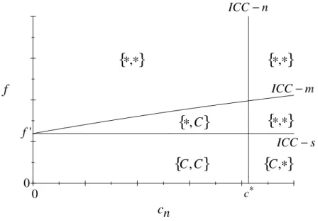
The equilibrium collusion pattern is illustrated in Figure 1, where the variable cost of the non-merged …rm cn is depicted on the x-axis and the
indivisible …xed cost of collusion f is depicted on the y-axis, and where is …xed.
The symmetric market structure. Let us …rst address the case where the non-merged …rm faces a zero variable production cost (recall that the merged …rm is assumed to have a zero variable production cost). ICC-s then depicts the indivisible …xed cost at which the merged …rm’s ICC (2) binds when the non-merged …rm also faces a zero production cost. We refer to this as f0, where f0 f (0; ). This curve is horizontal since in this case,
no …rm faces a positive variable production cost. It follows that collusion is sustainable in the symmetric market if f < f0.
The asymmetric market structure. Let us now turn to the case where the non-merged …rm faces a positive production cost, cn > 0. When
this is the case, ICC-n then depicts the production cost cn at which the
non-merged …rm’s ICC (3) binds. This curve is vertical since the non-non-merged …rm is assumed not to pay the per-period …xed indivisible cost. In addition, Assumptions 2 and 3 imply that ICC (3) holds only if cost asymmetries are su¢ ciently low, i.e., if cn< c .
Finally, ICC-m depicts the pairs (cn; f ) for which the merged …rm’s ICC
(2) binds. At cn = 0, this curve obviously coincides with the curve ICC-s.
The slope of the curve ICC-m is ambiguous, however.
In order to illustrate our …rst result, we make use of the following as-sumption, which implies that the ICC-m curve is upward sloping at cn = 0
and is never below ICC-s:
Assumption 4a f is weakly increasing in cn and @c@fn > 0 cn=0
.
Assumption 4a is shown to hold in the DPB model under several as-sumptions on how …rms share pro…ts in the collusive phase:13 (i) the joint
pro…t-maximizing (JPM) cartel, where …rms choose prices or quantities to 13See Appendices B and C.
0.0 0.1 0.2 0.3 0.4 0.5 0.0 0.1 0.2 0.3 0.4 n
c
f
' f 0 0 c∗ n ICC − m ICC− s ICC−{ }
∗,∗{ }
∗,∗{ }
∗,∗{ }
∗,C{ }
C,∗{ }
C,CFigure 1: Equilibrium Collusion Pattern: ICC-m upward sloping
maximize joint pro…ts, and (ii) the equal price increase cartel, where each …rm increases its price by an equal amount from the non-collusive equilibrium price.
Clearly, there will be collusion in this asymmetric market structure if and only if we are below the ICC-m curve and to the left of the ICC-n curve. So, we can now characterize the equilibrium collusion pattern under Assumptions 1-3 and 4a. This is done in Figure 1, where fC; g indicates that collusion can be sustained in the symmetric market structure but not in the asymmetric market structure, f ; Cg indicates that collusion cannot be sustained in the symmetric market structure but can be sustained in the asymmetric market structure, etc.
We speci…cally note that there exist parameter values in the DPB model under the joint pro…t-maximizing rule or the equal price increase rule such that Figure 1 is valid. We derive Figure 1 from the DPB model in Appendices B and C1. Now, using Figure 1 we have the following result:
Proposition 1 Under Assumptions 1-3 and 4a, and at a …xed indivisible cost so high that no collusion can be sustained in the symmetric case (f > f0),
there exists a …xed indivisible cost such that (i) …rms do not collude for low asymmetries; (ii) …rms collude for intermediate asymmetries; and (iii) …rms do not collude for large asymmetries.
Proof. Let f = f0 + (i.e. ICC-s does not hold), where is arbitrarily
small and positive and let c0 denote the value of c
n for which the ICC-m
binds with equality at f = f0 + . Then, there exist (i) ci < c0 such that
ICC-m does not hold; (ii) cii 2 (c0; c ) such that the ICC-m and the ICC-n
hold; and (iii) ciii > c such that ICC-n does not hold.
This result thus shows that there exist levels for the …xed indivisible cost of collusion such that (i) …rms do not collude when asymmetries are small; (ii) …rms do collude when asymmetries are moderate; and (iii) …rms do not collude when asymmetries are large. The intuition is simple. For collusion to arise, …rms cannot be too symmetric since the largest (most e¢ cient) …rm will then not have the incentive to cover the …xed indivisible cost of collusion.14. On the other hand, …rms cannot be too asymmetric either, for if there are strong asymmetries, the smallest …rm in the collusive agreement will have strong incentives to deviate from the collusive conduct and steal the business of its rival.
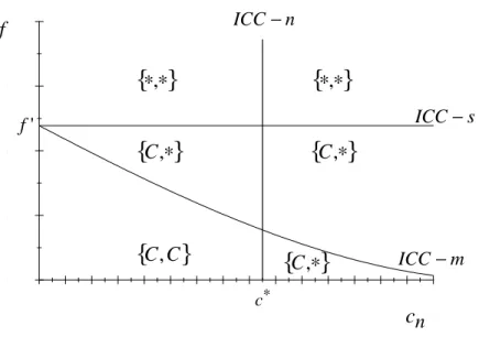
To illustrate our second result, we now make use of the following assump-tion, which implies that the ICC-m curve is downward sloping at cn= 0 and
is never above ICC-s:
Assumption 4b f is weakly decreasing in cn and @c@f
n < 0 c n=0
.
Assumption 4b is shown to hold in the DPB model under the constant market shares rule (see Appendix C2), where …rms reduce prices keeping market shares constant, i.e. equal to the market shares in the Bertrand-Nash equilibrium. We can now characterize the equilibrium collusion pattern under Assumptions 1-3 and 4b. Using Figure 2, we can then derive the following result:
Proposition 2 Under Assumptions 1-3 and 4b, and at such a low …xed in-divisible cost that collusion can be sustained in the symmetric case (f < f0), there exist levels for the …xed indivisible cost such that (i) …rms collude for small asymmetries; and (ii) …rms do not collude for large asymmetries.
14Remember that under the joint pro…t-maximizing or the equal price increase rule, this
0.0 0.1 0.2 0.3 0.4 0.5 0.6 0.7 0.8 0.9 1.0 1.1 1.2 1.3 1.4 1.5 0.000 0.005 0.010 0.015 0.020
f
nc
n ICC− m ICC− s ICC− ' f ∗ c{ }
∗,∗{ }
∗,∗{ }
C,∗{ }
C,∗{ }
C,C{ }
C,∗Figure 2: Equilibrium Collusion Pattern: ICC-m downward sloping
Proof. Let f = f0 ", where " is arbitrarily small and positive, and letec0
denote the value of cn for which the ICC-m binds with equality at f = f0 ".
Then, there exist (i)eci <ec0 such that ICC-m and ICC-n hold; and (ii)ecii >ec0
such that ICC-m does not hold.
This result thus shows that there exist levels for the …xed indivisible cost of collusion such that (i) …rms collude when asymmetries are minimal but do not collude when asymmetries are larger. For collusion to arise, …rms cannot be too asymmetric, otherwise the largest (most e¢ cient) …rm will not have the incentive to cover the …xed indivisible cost of collusion since it bene…ts less from the cartel being formed under the constant market share rule. Moreover, …rms cannot be too asymmetric for another reason. If there are strong asymmetries, the smallest …rm in the collusive agreement will have strong incentives to deviate from the collusive conduct and steal the business from its rival.15
15Note that it can be shown that the non-merged (ine¢ cient) …rms will have a lower
2.2
Stage 1: The merger model
In order to determine the merger pattern, we make use of an endogenous merger model developed by Horn and Persson (2001a) where the merger for-mation is treated as a cooperative game of coalition forfor-mation. The merger model has three basic components: (i) a speci…cation of the owners determin-ing whether one ownership structure Mi dominates another structure; (ii) a
criterion for determining when these owners prefer the former structure to the latter; and (iii) a stability (solution) criterion that selects the ownership structures seen as solutions to the merger formation game on basis of all pairwise dominance rankings.
The dominance relation is such that for some market structure Mj to
dominate or block another structure Mi, all owners involved in forming and
breaking up mergers between the two structures in some sense prefer the dominating structure to the other structure. Which owners are then able to in‡uence whether Mj dominates Mi? Owners belonging to identical
coali-tions in the two structures cannot a¤ect whether Mj will be formed instead of Mi, since payments between coalitions are not allowed. But all
remain-ing owners can in‡uence this choice. Owners who are linked this way in a dominance ranking between two structures Mi and Mj belong to the same decisive group of owners with respect to market structures Mi and Mj,
de-noted by Dij
g. The formal de…nition of a decisive group may appear somewhat
opaque.16 However, the concept itself is straightforward and, in “practice”, it is very easy to …nd the decisive groups. For instance, in a dominance rank-ing of MD =
f12; 3g and MT =
f1; 2; 3g; owner 3 belongs to identical …rms in both structures and hence, is not decisive. The only decisive group with respect to these two structures is hence DDT
1 = f1; 2g: Or, in a dominance
ranking of MD =
f12; 3g and MM =
f123g, owners 1, 2 and 3 belong to di¤erent …rms in the two structures. Hence, all three owners belong to a decisive group. The decisive groups are thus DDM
1 =f1; 2; 3g.
Mj dominates Mi via a decisive group if and only if the combined pro…t
of the decisive group is larger in Mj than in Mi. But, with more than one decisive group, these groups may dominate in opposite directions. It is therefore required that for Mj to dominate Mi, written Mj dom Mi,
domination holds for each decisive group with respect to Mi and Mj: The de…nition of decisive groups and the dom relation describes how to rank any pair of ownership structures. It remains to specify how these
rankings should be employed in order to predict the outcome of the merger formation. To this end, de…ne those structures that are undominated, i.e., that are in the core, as Equilibrium Ownership Structures (EOS).
To our knowledge, all papers on mergers and cartels have treated the merger decision as exogenous, not determining the equilibrium merger. The focus of this section will be to identify the equilibrium merger under two di¤erent merger policies. The …rst is a laissez-faire policy where all two-…rm mergers are allowed, but a merger to monopoly is forbidden. The second is an anti-symmetric merger policy, where no mergers leading to symmetric industry structures are allowed.
We can then derive the following Lemma:
Lemma 1 Under the laissez-faire policy, the equilibrium merger gives rise to the highest aggregate duopoly pro…t.
Proof. This follows from Proposition 2 in Horn and Persson (2001a) and from the fact that, in our model, the pro…t ‡ows both under collusion and non-collusion regimes are time invariant.
Recall that we have assumed c1 = c and c2 = c3 = 0: So, the marginal
costs associated with the possible merged entities are c12 = c13 = c23 = 0.
Let MA denote the market structure following a merger between …rm 1 and
…rm 3, referred to as a merger to symmetry, and MB denote the market structure following a merger between …rms 2 and 3, referred to as a merger to asymmetry. We can then state that a merger to symmetry will take place if and only if the following condition holds:
Ah= Ah m + Ah n > Bk m + Bk n = Bk; (5) where h; k = ; C.
Using condition (5), Figure 1 and the DPB model we can then derive the following result:
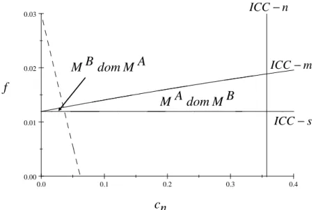
Proposition 3 An anti-symmetric merger policy (blocking mergers to a sym-metric market structure) can induce a merger without cost synergies (i.e. be-tween …rm 2 and …rm 3), yielding a higher average production cost and a lower aggregated producer and consumer surplus.
0.0 0.1 0.2 0.3 0.4 0.00 0.01 0.02 0.03
f
nc
n ICC− m ICC− s ICC−A
M
dom
B
M
B
M
dom
A
M
Figure 3: Equilibrium Mergers
This result can be illustrated in Figure 3, which builds on Figure 1 and where the merger condition (5) is included. In what follows, let us focus the attention on the region of Figure 1 where ICC-m and ICC-n hold but ICC-s does not. Then, consider the merger condition (5) which in this case becomes: Ah= A m = A n > BC m + BC n = Bh; (6)
since in this region, …rms will not collude in the symmetric market structure MA but will be able to collude in the asymmetric market structure MB (see
Figure 1). The downward sloping dashed line represents merger condition (6) when it is binding. This dashed line divides the region under consideration into two di¤erent subregions. In the right subregion, MA dominates MB,
whereas the opposite holds in the left subregion.
It is important to note at this point that in the whole region under analy-sis, …rms will not be able to collude in case a merger results in a perfectly symmetric market structure. Therefore, the reason why the symmetric mar-ket structure MA dominates the asymmetric market structure MB in the
to symmetry results in collusion amongst the remaining …rms in the mar-ket. Instead, what drives this result is that this merger will give rise to very signi…cant savings on industry costs.
So, by adopting an anti-symmetry merger policy, antitrust authorities force …rms to opt for the merger leading to the asymmetric market struc-ture, MB. This alternative merger will, in the region under analysis, create
the most favorable conditions for collusion to arise since asymmetries between the two remaining …rms are moderate after the merger (see Proposition 1 and Figure 1). In addition, for some parameter values, the gains from successful collusion which are obtained in this asymmetric industry structure are so high that they will more than compensate for the fact that one of the collud-ing …rms has high production costs. Consequently, by forbiddcollud-ing a merger leading to a symmetric industry structure, competition authorities may end up with a merger that does not only create lower industry cost savings, but also facilitates collusion.
3
Endogenous indivisible cost of cartelization
We here provide an example of an endogenous indivisible cost of creating and maintaining a cartel. As described in the Introduction, in 1987, Brown Boveri Company (later ABB) embarked on a strategic program for acquiring district heating pipe producers across Europe. However, this program was considered to be unfairly costly as indicated by the following quote from §28 of the EC Decision: “ABB for its part considers that it was unfairly having to bear all the cost of industry reorganization while other producers obtained a free ride.” Moreover, in reaction to the Powerpipe’s (the cartel outsider) aggressive behavior and entry into new geographical markets, ABB decided to use several predatory strategies to protect the cartel.
To capture this process of creating and maintaining the cartel, consider the following modi…ed model set-up, where we keep the repeated oligopoly game we had before but change period 1’s interaction in the following way. Now, …rm 3 is outside the cartel market and contemplates entering it. The cartel might prevent this entry by buying out the potential entrant. To this end, we assume that the e¢ cient …rm, …rm 2, makes a take-it-or-leave-it o¤er to …rm 3.
There are two scenarios to consider, one with an acquisition and one without an acquisition:
Case 1: No buyout. In this case, …rm 3 enters the market facing a variable cost c3. It is assumed that if entry occurs, collusion is not
sus-tainable and …rms compete à la Bertrand in each period, generating pro…ts
B
1 (c1; c2; c3), B2 (c1; c2; c3), and B3 (c1; c2; c3), respectively. This assumption
of one-shot Bertrand competition could be supported by the fact that collu-sion is not sustainable with three …rms in the market or by …rm 3 deciding to denounce the existence of the collusive agreement to the antitrust authorities about the illegal behavior upon entering the market.17
Case 2: A buyout takes place. To focus on the buyout as an in-divisible collusion cost, we assume that a buyout would not be pro…table if collusion did not occur post buyout. We can then use the above set-up to determine whether there will be collusion, taking the indivisible buyout cost A into account. It immediately follows that if a buyout takes place in equilibrium, …rm 2 will make an o¤er equal to …rm 3’s reservation price, i.e. its pro…t if it enters. The ICC for …rm 2 is then given by:
1 X t=0 C 2 p C 2; p C 1; c1; c2 A t> 2 p2 p C 1 ; p C 1; c1; c2 + 1 X t=1 2 pB2; p B 1; c1; c2 t; (7) where the indivisible acquisition cost A = B3 (c1; c2; c3) is the reservation
price of …rm 3. The ICC for …rm 1 is given by
1 X t=0 C 1 p C 1; p C 2; c1; c2 t> 1 p1 p C 2 ; p C 2; c1; c2 + 1 X t=1 1 pB1; p B 2; c1; c2 t: (8) To simplify the presentation, we assume the buyout price A to be inde-pendent of the level of asymmetry, i.e. A = B
3 (c1; c2; c3) = A. Consequently,
it is assumed that if c1 decreases, c2 will increase in such a way that the
ac-quisition price will not change. Then, using assumptions A1, A2, A3, and A4a, it directly follows that we can make use of the graphical solution in Figure 1 to describe the equilibrium, where in the horizontal axis we have c1
(the marginal cost of the outsider to the merger) and in the vertical axis we now represent A (instead of f ).
What will then happen if we relax the assumption that the acquisition price is independent of the cost asymmetry? If the buyout price (reservation
price) decreases in asymmetries, collusion becomes relatively more likely un-der asymmetry, whereas the opposite is true if the buyout price increases in asymmetries.
We then make use of the DPB model to show the existence of an equi-librium where the buyout of a collusion breaking potential entrant will be undertaken if and only if the market structure is medium asymmetric. Thus, we can show that:
Proposition 4 There exist parameter values in the DPB model under the joint pro…t-maximizing rule such that …rm 2 buys out …rm 3 if and only if collusion occurs post-buyout, which is the case if and only if the market structure is medium asymmetric.
Proof. See Appendix D.
4
Conclusion
In the existing literature, mergers leading to symmetric size distribution (cost structure) of …rms have been shown to increase the risk of collusion, since the asymmetry between …rms creates incentives to deviate both in the collusive phase and the punishment phase. Allowing for indivisible costs of collusion, which one …rm must bear, we show that forbidding mergers leading to sym-metric market structures can induce mergers leading to asymsym-metric market structures with higher production costs and a higher risk of collusion. In particular, we show that if the rule determining the collusive outcome has the property that the large (e¢ cient) …rm bene…ts su¢ ciently more from col-lusion when industry asymmetries increase, colcol-lusion can become more likely when …rms are asymmetric.
These results thus suggest the importance of studying the environment for post merger collusion in detail, taking into account the role played by a potential ring-leader in the collusion process.
The key to our result is the chosen rule for determining the collusive outcome. If the cartel behavior rule has the property that the gains of the large (e¢ cient) …rm from collusion increase with industry asymmetries, our main results are valid. Basically, what is important is that the “advantages” of the large (e¢ cient) …rm in the non-cooperative interaction (e.g. its larger market share, lower production costs, larger capital stock, or higher quality products) are used to give leverage in capturing more of the surplus created
in the collusive outcome. This will be the case for some particular rules of how to determine the cartel outcome. As shown above, a rule with this characteristic is the joint pro…t maximization rule in the DPB model. But this rule has some problematic features, as discussed in Harrington (2004). In particular, it could allocate the gains from collusion very unevenly.
Notice, however, that the constant market share rule, which is one of the most frequently used allocation rules, also has some odd features in our setting: the small (ine¢ cient) …rm gains more from collusion than the large (e¢ cient) …rm. The reason is that under the constant market share rule, the large (e¢ cient) …rm is forced to reduce output much more than the small (ine¢ cient) …rm which implies that the “cost” due to the output reduction to a larger extent falls on this large (e¢ cient) …rm.18 This rule is evidently
used in practice, but this property suggests that other rules should be used in practice where the large (e¢ cient) …rm gains most from collusion. For example, we show that the large (e¢ cient) …rm gains most from collusion under an equal price increase rule. However, more research is needed to better understand which rules are used in what context and what are their implications for mergers and cartel policies.
References
[1] Compte, O., Jenny, F. and Rey, P. (2002), “Capacity Constraints, Merg-ers and Collusion”, European Economic Review, Vol. 46, 1-29.
[2] Dick, A. R., 2003, Coordinated interaction: pre-merger constraints and post-merger e¤ects”, Geo.MasonL.Rev, Vol. 12:1.
[3] Friedman, J. W. (1971), “A Non-cooperative Equilibrium for Su-pergames”, Review of Economic Studies 28, 1-12.
[4] Harrington, J. (2004), Encore Lectures on the
Eco-nomics of Collusion, available for download at:
http://www.econ.jhu.edu/People/Harrington/ENCORELectures.pdf. [5] Harrington, J. (2006), “How do Cartels Operate?”, Foundations and
Trends in Microeconomics, Vol. 2(1), pp. 1-105.
[6] Horn, H and Persson, L., 2001a, ”Endogenous Mergers in Concentrated markets”, International Journal Industrial Organization, vol 19, NO. 8, 1213-1244.
[7] Horn, H and Persson, L., 2001b, “The Equilibrium Ownership of an International Oligopoly,” Journal of International Economics, Vol. 53, No. 2.
[8] Leveinstein, M. C., and Suslow, V. S., 2006, ”What determines cartel success?”, Journal of Economic Literature, Vol. XLIV, pp. 43-95. [9] Lommerud, K.E., Straume O.R. and Sorgard, L., 2006, ”National versus
international mergers in unionized oligopoly,” RAND Journal of Eco-nomics, 37, 212-233.
[10] Motta, M. (2004) Competition Policy. Theory and Practice. Cambridge University Press.
[11] Norback, P.-J. and Persson, L. (2006), “Entrepreneurial Innovations, Competition and Competition Policy”, Working Paper No. 670, Re-search Institute of Industrial Economics.
[12] Rothschild, R. (1999) "Cartel stability when costs are heterogeneous", International Journal of Industrial Organization,Volume 17, Issue 5, July, 717-734
[13] Singh, N. and Vives, X. (1984), “Price and Quantity competition in a Di¤erentiated Duopoly”, RAND Journal of Economics, Vol. 15 No. 4, 546-554.
[14] Vasconcelos, H. (2005) “Tacit Collusion, Cost Asymmetries, and Merg-ers”, RAND Journal of Economics, Vol. 36 No. 1, 39-62.
[15] Verboven, F (1997) “Collusive Behavior with Heterogeneous Firms,” Journal of Economic Behavior and Organization, 33(1), 21-36.
A
The DPB model
Consider an in…nitely repeated game with two …rms, denoted with sub-scripts i = 1; 2. Each …rm produces a single variety of a good X and the quantity of variety i is denoted qi. The …xed costs of production are taken
to be zero and …rm i’s constant marginal cost is given by ci. Let c1 = 0 and
c2 = c > 0:
Following Singh and Vives (1984), we assume that a representative con-sumer maximizes the following utility function:
U (q1; q2) = a1q1+ a2q2
1 2 b1q
2
1 + b2q22+ 2 q1q2 + y; (9)
where y is a numeraire ‘outside’ good. This utility function gives rise to a linear demand structure, where direct demands can be written as:
q1(p1; p2) = 1 1p1+ p2 (10)
q2(p1; p2) = 2 2p2+ p1; (11)
where d b1b2 2 ; i (aibj aj ) =d; i bj=d for i 6= j, i = 1; 2, and
=d.
Firms compete in prices. Every period of time can be divided into the following stages: …rms …rst set prices, consumers then determine the demand for the two varieties of the good and, …nally, markets clear.
The pro…t of …rm i is i = P1t=0 t ti(pt1; pt2), where pti is the price
charged by …rm i in period t and …rm i’s individual pro…t in period t is
i pt1; p t 2 = qi pt1; p t 2 p t i ci : (12)
A.1
Non-cooperative behavior and joint pro…t
maxi-mization
Consider a single period game. If the …rms play noncooperatively, each …rm solves the following optimization problem
max
pi
qi(p1; p2) (pi ci) : (13)
From the …rst-order conditions (FOCs) of the previous maximization prob-lem, it can be concluded that the (positively sloped) reaction functions of …rms 1 and 2 are, respectively, given by:
p1(p2) =
1+ p2
p2(p1) =
2+ 2c + p1
2 2 : (15)
Now, some algebra shows that in the unique Bertrand-Nash equilibrium of the one-shot game, …rms’prices and individual pro…ts are:
pB1 = 2 1 2+ 2 + 2 c 4 1 2 2 ; (16) pB2 = 2 2 1+ 1 + 2 1 2c 4 1 2 2 ; (17) 1 pB1; pB2 = 1(pB1)2; (18) 2 pB1; p B 2 = 2 2 2 1+ 1 + c ( 2 2 1 2) 4 1 2 2 2 : (19)
If …rms instead decide to maximize their joint pro…t in the one-shot game, their equilibrium prices result from the following optimization problem:
max p1;p2 2 X i=1 qi(p1; p2) (pi ci) : (20)
From the FOCs of the previous maximization problem, and after some re-arranging, it is concluded that the cooperative prices of …rms 1 and 2 are, respectively, given by:
pC1 = 2 + 1 2
2 ( 1 2 2); (21)
pC2 = 2 1+ 1 + c ( 1 2
2)
2 ( 1 2 2) : (22)
In addition, …rms’collusive equilibrium pro…ts are:
1 pC1; p C 2 = ( 1+ c ) ( 2 + 1 2) 4 ( 1 2 2) ; (23) 2 pC1; p C 2 = ( 2 c 2) ( 2 1+ 1 + c ( 2 1 2)) 4 ( 1 2 2) : (24)
A.2
Deviation pro…ts
If a given …rm is considering deviating in period t, when …rms are supposed to set prices (21) and (22) then, making use of …rms’reaction functions (14) and (15), it may be concluded that each …rm’s optimal deviation price is given by: p1 pC2 = 1(2 1 2 2) + 2 1 c ( 2 1 2) 4 1( 1 2 2) ; (25) and p2 pC1 = 2(2 1 2 2) + 1 2 2c 2( 2 1 2) 4 2( 1 2 2) : (26)
Hence, the corresponding deviation pro…ts for …rms 1 and 2 are, respec-tively, given by:
1 p1 p C 2 ; p C 2 = 1 p1 p C 2 2 ; (27) 2 pC1; p2 p C 1 = ( 2(2 1 2 2) + 1 2+ 2 2c ( 2 1 2)) 2 16 2( 2 1 2) 2 : (28)
B
Generating Figures 1 and 3 and proving
Propositions 1 and 3
In what follows, let 1 = 2 = 1 = 2 = 1 and = 1=3.
B.1
Deriving Figure 1
B.1.1 Curve ICC-s
Making use of eqs. (4), (18), (23), (27), some algebra shows that: f0 = f (0; ) = 3 8 (1 ) 25 64 9 25: (29)
For a given (and su¢ ciently high) value of the discount factor , the previous equation is represented by the horizontal line ICC-s in Figure 1.
B.1.2 Curve ICC-n
Making use of eqs. (3), (19), (24) and (28), and after some rearranging, it may be concluded that condition (3) becomes:
(1 cn) (3 2cn) 8 1 1 > (5 4cn)2 64 + (21 17cn)2 1225 1 : (30)
Now, for a given value of , the value of cn for which the previous condition
binds is represented by the vertical line ICC-n in Figure 1.
B.1.3 Curve ICC-m
Combining the results in eqs. (4), (18), (23), (27), it may be concluded that: f (cn; ) = 1 8(cn+ 3) (1 ) (2cn+ 15)2 576 9 (cn+ 7)2 1225 : (31)
For a given , the previous condition is represented by the ICC-m curve in Figure 1.
So, this section proves that there exist parameter values in the DPB model such that Figure 1 is valid, as claimed in Proposition 1.
B.2
Deriving Figure 3
In Figure 3, we assume that = 0:9. This being the case and making use of eqs. (29), it is straightforward to show that the equations representing the ICC-s, the ICC-n and the ICC-m curves are, respectively, given by:
f0 = f (0; 0:9) = 0:011938; (32) c = 0:35742; (33) f (cn; 0:9) = 1 8(cn+ 3) 0:1 (2cn+ 15) 2 576 8:1 (cn+ 7) 2 1225 : (34)
Consider now the region in Figure 1 where ICC-m and ICC-n hold, but ICC-s does not. In this region, …rms will not collude in the symmetric market structure MA. Hence, making use of eqs. (18)-(19), it can easily be concluded
that in this symmetric market structure, the present discounted value of individual …rms’pro…ts and the industry pro…t is, respectively, given by:
A m = A n = 9 25 1 1 ; (35)
A = 18
25 1
1 : (36)
On the other hand, and restricting the attention to the same region of para-meter values, it is shown that …rms will be able to collude in the asymmetric market structure MB. Therefore, making use of eqs. (23)-(24), it is concluded
that in the asymmetric market structure, the present discounted value of in-dividual …rms’pro…ts and the industry pro…t is, respectively, given by:
BC m = 1 8(cn+ 3) f 1 1 ; (37) BC n = 1 8(1 cn) (3 2cn) 1 1 ; (38) BC = c2n 2cn+ 3 4 f 1 1 : (39)
Now, making use of eqs. (36) and (39), it may be concluded that the merger condition A > BC (see eq. (5)) boils down to:
f > c 2 n 2cn+ 3 4 18 25: (40)
The previous eq. is represented by the dashed line in Figure 3.
Finally, we need to check whether the prices charged by the merged entity and the non-merged …rm are higher in market structure MB than in market
structure MA. Regarding the merged entity (…rm m), making use of eqs.
(16) and (21), it is easy to check that it will charge higher prices in case the ex-post merger market structure is MB, since:
pAm = 3 5 < p BC m = 3 4: (41)
As for the non merged entity (…rm n), making use of eqs. (17) and (22), it is simple to check that it will also set a higher price in market structure MB
than in market structure MA, since:
pAn = 3 5 < p BC n = 1 4(2cn+ 3) ; (42)
which is true for any cn > 0. Hence, a merger leading to an asymmetric
market structure MB will, in the region under consideration, give rise to a
lower consumer surplus than a merger leading to a completely symmetric industry structure, MA. This completes the proof of Proposition 3.
C
Alternative cartel behavior rules
In Appendices A and B, joint pro…t maximization was used as a criterion for selecting the collusive outcome. This section studies the properties of two other alternative cartel behavior rules which have been used in practice: the equal price increase rule and the constant market shares rule.
As before, we focus the attention on a speci…c parametrization of the DPB model where 1 = 2 = 1 = 2 = 1 and = 1=3. This being the case,
from eqs. (16), (18) and (19), it may be concluded that the Bertrand-Nash equilibrium pro…ts are given by:
1 pB1; p B 2; c = 9 (7 + c)2 1225 ; (43) 2 pB1; p B 2; c = (21 17c)2 1225 : (44)
C.1
The equal price increase rule
Suppose that along the collusive path, each …rm reduces its output by the same amount > 0 (leading to an equal price increase). Notice that …rm i’s optimal value of results from the following maximization problem:19
max 3 2 9 8 q B i 3 8 q B j ci qiB ; (45) where qB
i denotes …rm i’s quantity in the Bertrand-Nash equilibrium, i; j =
1; 2; i 6= j. It can easily be checked that the optimal values of for …rms 1 and 2 are, respectively, given by:
1 = 1 10+ 1 70c; (46) 2 = 1 10 17 210c: (47)
So, the two …rms in the cartel will have to bargain over the value of 2 [ 2; 1]. Assume that the chosen level of will be ( 2+ 1) =2. The
19Making use of eqs. (10)-(11), it is straightforward to conclude that, for the
spe-ci…c parameter values we have chosen, …rm i’s inverse demand function is given by pi= 3=2 9=8qi 3=8qj:
corresponding cooperative prices and pro…ts are then given by: b pC1 = 3 4 + 1 28c; (48) b pC2 = 3 4 + 13 28c; (49) bC1 = (21 + c) (21 + 5c) 1176 ; (50) bC2 = (7 5c) (21 19c) 392 : (51)
Now, making use of eqs. (14), (15), (48) and (49), it is shown that the optimal deviation prices for …rms 1 and 2 are, respectively, given by:
p1 pbC2 = 5 8+ 13 168c; (52) p2 pbC1 = 5 8+ 85 168c: (53)
The corresponding optimal deviation pro…ts are: bD1 = (105 + 13c)2 28 224 ; (54) bD2 = (105 83c)2 28 224 : (55)
So, combining eqs. (4), (43), (50) and (54), it may be concluded that
f (cn; ) = (21 + cn) (21 + 5cn) 1176 (1 ) (105 + 13cn) 2 28 224 9 (7 + cn) 2 1225 : (56) Now, it can easily be checked that, for a given value of (say = 0:9), f (cn; ) increases in cn in the relevant region of parameter values. So, the
previous condition can be represented by such an upward sloping ICC-m curve as that presented in Figure 1.
C.2
The constant market shares rule
Suppose that along the collusive path, …rm i’s output is qC
i = qiB, where qBi
denotes …rm i’s quantity in the Bertrand-Nash equilibrium, i; j = 1; 2; i 6= j, and 2 (0; 1). When this is the case, each …rm’s market share along the collusive path coincides with its market share at the Bertrand Nash equilibrium. The problem, however, is to identify the value of chosen by the cartel.
Notice that …rm i’s optimal value of results from the following maxi-mization problem: max 3 2 9 8 q B i 3 8 q B j ci qiB: (57)
It can easily be checked that the optimal values of for …rms 1 and 2 are, respectively, given by:
1 = 35 2 (21 2c); (58) 2 = 35 18 3 2c 7 4c: (59)
So, the two …rms in the cartel will have to bargain over the value of 2 [ 2; 1]. Let the chosen level of bee1.20 The corresponding cooperative
prices and pro…ts are then given by: e pC1 = 3 4; (60) e pC2 = 3 4 21 + 8c 21 2c; (61) eC1 = 9 8 7 + c 21 2c; (62) eC2 = 1 8 (21 17c) (8c2 60c + 63) (21 2c)2 : (63)
Now, making use of eqs. (14), (15), (60) and (61), it is shown that optimal deviation prices for …rms 1 and 2 are, respectively, given by:
p1 peC2 = 105
8 (21 2c); (64)
20Since we have assumed the most e¢ cient …rm to be the one which must cover
indi-visible per-period coordination …xed costs, it may be natural to assume that it has all the bargaining power in the choice of .
p2(p1) =
5 8 +
1
2c: (65)
The corresponding optimal deviation pro…ts are: eD1 = 11 025 64 (21 2c)2; (66) eD 2 = (5 4c)2 64 : (67) C.2.1 Deriving Figure 2
Curve ICC-s Making use of eqs. (4), (43), (62) and (66), some algebra shows that: f0 = f (0; ) = 9 8 7 21 (1 ) 11 025 64 (21)2 9 (7)2 1225: (68)
For a given (and su¢ ciently high) value of , the previous equation is repre-sented by the horizontal line ICC-s in Figure 2.
Curve ICC-n Making use of eqs. (44), (63) and (67), it may be concluded that condition (3) can be rewritten as:
1 1 1 8 (21 17cn) (8c2n 60cn+ 63) (21 2cn) 2 > (5 4cn)2 64 + (21 17cn)2 1225 1 : (69) For a given value of , the value of cn for which the previous constraint
is binding is represented by the vertical line ICC-n in Figure 2.
Curve ICC-m Combining the results in eqs. (4), (43), (62) and (66), it may be concluded that:
f (cn; ) = 9 8 7 + cn 21 2cn (1 ) 11 025 64 (21 2cn)2 9 (7 + cn) 2 1225 : (70)
It can easily be checked that for a given su¢ ciently high value of the discount factor , f (cn; ) decreases in cn. So, the previous condition is represented
D
Proof of Proposition 4
Take the speci…c parametrization of the DPB model used above, where 1 = 2 = 1 = 2 = 1 and = 1=3.
If the two …rms, whose constant marginal costs are c1 and c2; play
non-cooperatively, then it is easily shown that their Bertrand-Nash equilibrium pro…ts are given by:
B 1 (c1; c2) = 1 1225(21 17c1+ 3c2) 2 ; (71) B 2 (c1; c2) = 1 1225(21 + 3c1 17c2) 2 : (72)
If …rms instead decide to maximize their joint pro…t in the one-shot game, their equilibrium pro…ts will be as follows:21
C 1 (c1; c2) = 1 24(3c1 c2 3) (2c1 3) ; (73) C 2 (c1; c2) = 1 24(3c2 c1 3) (2c2 3) : (74)
Some algebra also shows that …rms’deviation pro…ts are equal to:
D 1 (c1; c2) = 1 576(12c1 2c2 15) 2 ; (75) D 2 (c1; c2) = 1 576(12c2 2c1 15) 2 : (76)
Now, making use of eq. (7), it may be concluded that the maximum acquisition cost eA that …rm 2 would be willing to pay is the one for which the ICC (7) is binding, i.e.,
e A = C2 pC2; pC1; c1; c2 (1 ) 2 p2 p C 1 ; p C 1; c1; c2 2 pB2; p B 1; c1; c2 ; (77) which, making use of eqs. (71)-(76), can, for the speci…c parametrization of the DPB model we have been using throughout the paper, be rewritten as:
e A (c1; c2; ) = 1 24(3c2 c1 3) (2c2 3) (1 ) 1 576(12c2 2c1 15) 2 (78) 1 1225(21 + 3c1 17c2) 2 : 21If c
Now, while the previous equation puts forward the threshold value for the acquisition price, the actual acquisition price is A = B3 (c1; c2; c3). For
the speci…c parametrization of the DPB model we are using, it is straightfor-ward to show that …rm 3’s individual (triopoly) pro…ts in a Bertrand-Nash equilibrium are given by:
B
3 (c1; c2; c3) =
(13c3 3c1 3c2 21)2
784 F3 A(c1; c2; c3); (79) where F3 0 denotes …rm 3’s …xed costs of production.
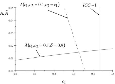
Consider now an example where = 0:9, c2 = 0:1, c3 = c1 and F3 = 0:4.
Figure 4 then presents the threshold acquisition price eA (c1; c2 = 0:1; = 0:9)
(solid upward sloping curve) and the actual acquisition price A(c1; c2 =
0:1; c3 = c1) (dashed downward sloping curve). So, …rm 2 will decide to
buy out …rm 3 and collude after this buyout in the region where the dashed decreasing curve is below the solid upward sloping curve (so that the actual price paid to acquire …rm 3 is lower than the maximum threshold price eA identi…ed above). In addition, Figure 4 also presents a vertical line which represents …rm 1’s ICC (eq. (8)), which making use of eqs. (71), (73) and (79) and for the speci…c parametrization of the model we are using in this example, implies that …rm 1 will decide to collude if c1 0:43360.
So, clearly, …rm 2 will decide to buy out …rm 3 and collusion between …rms 1 and 2 will take place in the market structure induced by this buyout if costs are medium asymmetric. This completes the proof of Proposition 4.
0.0 0.1 0.2 0.3 0.4 0.5 0.00 0.01 0.02 0.03 0.04 0.05 1