Are people aware of the Taylor rule?

(1)

Are People Aware of the Taylor Rule?

Carlos Carvalho

FRBNY

Fernanda Nechio

FRBSF

May 2011

The views expressed in this paper are those of the authors and do not necessarily re‡ect the position of the FRBNY, the FRBSF, or the Federal Reserve System.

(2)

Motivation

Most questions of interest to macroeconomists have a dynamic dimension

Main reason why issue of expectations formation is important

In particular, agents’understanding of policy is key (e.g. Taylor Principle)

Extense empirical literature on how monetary policy is conducted

(3)

This paper

“Are people aware of the Taylor rule?”

Idea: combine questions from the Michigan Survey about the future path of

t

(p

t

), i

t

, u

t

, and check for “consistency with Taylor rule”

– Example: P (i " j

"; u #) > P (i " j

#; u ")

Perform same analysis with

– Survey of Professional Forecasters

– Arti…cial surveys …lled in by VAR

(4)

What we …nd

Answers broadly consistent with awareness of Taylor rule

Degree of awareness not uniform across income and education levels

– Evidence that Fed’s dual mandate is:

understood by highest-income and college-degree households

not properly understood by lowest-income-quartile and

no-high-school-degree households

Break in (i

_t

;

_t

; u

_t

)

Taylor rule around 1987

– detected by highest-income and college-degree households

– undetected by lowest-income and no-high-school-degree households

(5)

Michigan Survey questions

About interest rates: “No one can say for sure, but what do you think will

happen to interest rates for borrowing money during the next 12 months–

will they go up, stay the same, or go down? ”

About unemployment: “How about people out of work during the coming

12 months–do you think that there will be more unemployment than now,

about the same, or less? ”

About prices

– “During the next 12 months, do you think that prices in general will go

up, or go down, or stay where they are now? ”, and

– “By about what percent do you expect prices to go (up/down) on the

average, during the next 12 months? ”

(6)

Assumptions

About interest rates:

– answers to an analogous question about direction of 3-month Treasury Bill

rate in 12 months would be the same

About unemployment

– pertains to civilian unemployment rate

About prices

– pertains to headline Consumer Price Index

– assume people know 12-month CPI in‡ation

– calculate predicted change in 12-month CPI in‡ation

– convert to “up/down/same”

(7)

Organizing framework

Start from

(8)

Organizing framework

Start from

i

_t

= r +

e _t _12;t

+

e_y

(y

_t

y

_tn

) + "

_t

Replace (y

_t

y

_tn

)

with

(u

_t

u

n_t

)

(with

<

0)

(9)

Organizing framework

Start from

i

_t

= r +

e _t _12;t

+

e_y

(y

_t

y

_tn

) + "

_t

Replace (y

_t

y

_tn

)

with

(u

_t

u

n_t

)

(with

<

0)

i

_t

= r +

_t _12;t

+

_u

(u

_t

u

n_t

) + "

_t

Subtract from E

_t

of 12-month lead, and assume var (u

n_t

) << var (u

_t

)

E

_t

i

_t+12

i

_t h

E

_{t t;t+12} _t _12;ti

+

_u

[E

_t

u

_t+12

u

_t

] +

e

"

_t

(10)

Taylor rule orderings

P (i " j

#; u ") <

(

P (i " j

#; u $)

P (i " j

$; u ")

)

< P (i ")

<

(

P (i " j

"; u $)

P (i " j

$; u #)

)

< P (i " j

"; u #) ;

(11)

Taylor rule orderings

P (i " j

#; u ") <

(

P (i " j

#; u $)

P (i " j

$; u ")

)

< P (i ")

<

(

P (i " j

"; u $)

P (i " j

$; u #)

)

< P (i " j

"; u #) ;

and

P (i # j

"; u #) <

(

P (i # j

"; u $)

P (i # j

$; u #)

)

< P (i #)

<

(

P (i # j

#; u $)

P (i # j

$; u ")

)

< P (i # j

#; u ") :

(12)

Partial e¤ects

Of in‡ation

P (i " j

#; u) < P (i " j

$; u) < P (i " j

"; u) ;

P (i # j

"; u) < P (i # j

$; u) < P (i # j

#; u) ;

(13)

Partial e¤ects

Of in‡ation

P (i " j

#; u) < P (i " j

$; u) < P (i " j

"; u) ;

P (i # j

"; u) < P (i # j

$; u) < P (i # j

#; u) ;

Of unemployment

P (i " j ; u ") < P (i " j ; u $) < P (i " j ; u #) ;

P (i # j ; u #) < P (i # j ; u $) < P (i # j ; u ") :

(14)

Estimated Taylor rule

OLS

IR

_t

=

₀

+

₁

Inf lation

_t

+

₂

U nemp

_t

+ u

_t

;

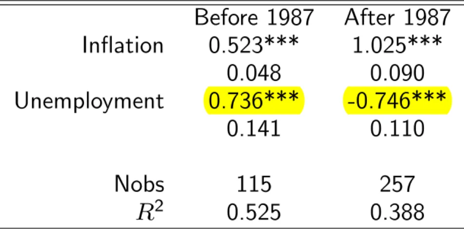
Table 1: Split-sample estimation

Before 1987 After 1987 In‡ation 0.523*** 1.025*** 0.048 0.090 Unemployment 0.736*** -0.746*** 0.141 0.110 Nobs 115 257 R2 0.525 0.388

(15)

Realized data

Table 2: Unconditional distributions

(%) – data

# $ " P (i) 56.03 - 43.94 P ( ) 45.53 - 54.47 P (u) 62.26 3.11 34.63

Table 3: Conditional distributions of i j ; u

(%) – data

# $ " Nobs P (i j "; u #) 19.78 - 80.22 91 P (i j "; u $) 100.00 - 0.00 3 P (i j "; u ") 100.00 - 0.00 46 P (i j #; u #) 43.48 - 56.52 69 P (i j #; u $) 80.00 - 20.00 5 P (i j #; u ") 100.00 - 0.00 43

(16)

Realized data

Table 4: Kolmogorov-Smirnov tests – data

Test statistic p-value (1) _{P (i) = P (i j} _{"; u #)} 0.363 0.000 (2) _{P (i) = P (i j} _{"; u ")} 0.440 0.000 (3) _{P (i) = P (i j} _{#; u #)} 0.126 0.300 (4) _{P (i) = P (i j} _{#; u ")} 0.440 0.000

(17)

Realized data

Table 5: Taylor rule orderings – data

Null Hypothesis t-stat p-value (1) _{P (i " j #; u ")} _{P (i ")} 14.17 0.00 (2) _{P (i ")} _{P (i " j "; u #)} 6.94 0.00 (3) _{P (i # j "; u #)} _{P (i #)} 6.94 0.00 (4) _{P (i #)} _{P (i # j #; u ")} 14.17 0.00

(18)

Realized data

Table 6: Partial e¤ects of in‡ation – data

Null Hypothesis mean di¤erence t-stat p-value P (i " j #; u #) P (i " j "; u #) 0.24 3.23 0.00 P (i " j #; u ") P (i " j "; u ") - - -P (i # j #; u #) P (i # j "; u #) 0.24 3.23 0.00 P (i # j #; u ") P (i # j "; u ") - -

-Table 7: Partial e¤ects of unemployment – data

Null Hypothesis mean di¤erence t-stat p-value P (i " j #; u ") P (i " j #; u #) 0.57 9.40 0.00 P (i " j "; u ") P (i " j "; u #) 0.80 19.10 0.00 P (i # j #; u #) P (i # j #; u ") 0.57 9.40 0.00 P (i # j "; u #) P (i # j "; u ") 0.80 19.10 0.00

(19)

Realized data

Table 8: Ordered probit – data

Estimates In‡ation 0.311***

0.104 Unemployment -1.829***

0.383

Table 9: Conditional distributions of i j ; u

(%) , ordered probit – data

# $ " (1) _{P (i j} _{"; u #)} 20.53 0.00 79.47 (2) _{P (i j} _{"; u $)} 84.29 0.00 15.71 (3) _{P (i j} _{"; u ")} 99.77 0.00 0.23 (4) _{P (i j} _{#; u #)} 42.07 0.00 57.93 (5) _{P (i j} _{#; u $)} 94.84 0.00 5.16 (6) _{P (i j} _{#; u ")} 99.97 0.00 0.03

(20)

Michigan Survey

Table 10: Unconditional distributions

(%) – Michigan Survey

# $ " P (i) 15.11 28.64 56.25 P ( ) 46.13 - 53.87 P (u) 13.84 50.69 35.48

Table 11: Conditional distributions of i j ; u

(%) , – Michigan Survey

# $ " Nobs (1) _{P (i j} _{"; u #)} 13.06 26.46 60.48 7,458 (2) _{P (i j} _{"; u $)} 11.16 28.90 59.94 28,465 (3) _{P (i j} _{"; u ")} 16.45 22.99 60.56 23,444 (4) _{P (i j} _{#; u #)} 15.46 33.01 51.53 7,852 (5) _{P (i j} _{#; u $)} 14.75 33.78 51.47 27,848 (6) _{P (i j} _{#; u ")} 21.74 26.49 51.77 15,772

(21)

Michigan Survey

Table 12: Kolmogorov-Smirnov tests – Michigan Survey

Test statistic p-value (1) _{P (i) = P (i j} _{"; u #)} 0.043 0.000 (2) _{P (i) = P (i j} _{"; u $)} 0.040 0.000 (3) _{P (i) = P (i j} _{"; u ")} 0.042 0.000 (4) _{P (i) = P (i j} _{#; u #)} 0.052 0.000 (5) _{P (i) = P (i j} _{#; u $)} 0.048 0.000 (6) _{P (i) = P (i j} _{#; u ")} 0.064 0.000

(22)

Michigan Survey

Table 13: Taylor rule orderings – Michigan Survey

Null Hypothesis mean di¤erence t-stat p-value (1) _{P (i " j #; u ")} _{P (i ")} 0.04 9.60 0.00 (2) _{P (i ")} _{P (i " j "; u #)} 0.04 6.57 0.00 (3) _{P (i # j "; u #)} _{P (i #)} 0.02 4.62 0.00 (4) _{P (i #)} _{P (i # j #; u ")} 0.07 17.48 0.00

(23)

Michigan Survey

Table 14: Partial e¤ects of in‡ation dropping i j ; u $ – Michigan Survey

Null Hypothesis mean di¤erence t-stat p-value P (i " j #; u #) P (i " j "; u #) 0.10 11.94 0.00 P (i " j #; u ") P (i " j "; u ") 0.09 16.81 0.00 P (i # j #; u #) P (i # j "; u #) 0.03 4.63 0.00 P (i # j #; u ") P (i # j "; u ") 0.05 12.39 0.00

Table 15: Partial e¤ects of unemployment dropping i j ; u $ – Michigan Survey

Null Hypothesis mean di¤erence t-stat p-value P (i " j #; u ") P (i " j #; u #) -0.01 -1.29 0.90 P (i " j "; u ") P (i " j "; u #) 0.00 0.07 0.47 P (i # j #; u #) P (i # j #; u ") 0.06 10.93 0.00 P (i # j "; u #) P (i # j "; u ") 0.03 7.24 0.00

(24)

SPF

Table 16: Unconditional distributions

(%) – SPF

# $ " P (i) 33.66 - 66.34 P ( ) 50.15 - 49.85 P (u) 44.06 0.15 55.79

Table 17: Unconditional distributions

(%) – SPF

# $ " Nobs P (i j "; u #) 16.06 - 83.94 654 P (i j "; u $) - - - 0 P (i j "; u ") 43.68 - 56.32 673 P (i j #; u #) 18.11 - 81.89 519 P (i j #; u $) 25.00 - 75.00 4 P (i j #; u ") 49.51 - 50.49 812

(25)

SPF

Table 18: Kolmogorov-Smirnov tests – SPF

Test statistic p-value (1) _{P (i) = P (i j} _{"; u #)} 0.176 0.000 (2) _{P (i) = P (i j} _{"; u ")} 0.100 0.000 (3) _{P (i) = P (i j} _{#; u #)} 0.155 0.000 (4) _{P (i) = P (i j} _{#; u ")} 0.158 0.000

(26)

SPF

Table 19: Partial e¤ects of in‡ation dropping i j ; u $ – SPF

Table 20: Partial e¤ects of unemployment dropping i j ; u $ – SPF

(27)

SPF

Table 21: Partial e¤ects of core in‡ation dropping i j ; u $ – SPF

(28)

VAR

Table 22: Unconditional distributions

(%) – VAR

# $ " P (i) 15.03 29.02 55.96 P ( ) 52.33 - 47.67 P (u) 13.47 50.78 35.75

Table 23: Conditional distributions of i j ; u

(%) , – VAR

# $ " Nobs (1) _{P (i j} _{"; u #)} 0.00 0.00 100.00 22 (2) _{P (i j} _{"; u $)} 0.00 13.16 86.84 38 (3) _{P (i j} _{"; u ")} 28.13 15.63 56.25 32 (4) _{P (i j} _{#; u #)} 0.00 0.00 100.00 4 (5) _{P (i j} _{#; u $)} 3.33 53.33 43.33 60 (6) _{P (i j} _{#; u ")} 48.65 37.84 13.51 37

(29)

VAR

Table 24: Kolmogorov-Smirnov tests – VAR

Test statistic p-value (1) _{P (i) = P (i j} _{"; u #)} 0.440 0.000 (2) _{P (i) = P (i j} _{"; u $)} 0.309 0.003 (3) _{P (i) = P (i j} _{"; u ")} 0.131 0.659 (4) _{P (i) = P (i j} _{#; u #)} 0.440 0.281 (5) _{P (i) = P (i j} _{#; u $)} 0.126 0.392 (6) _{P (i) = P (i j} _{#; u ")} 0.424 0.000

(30)

VAR

Table 25: Taylor rule orderings – VAR

Null Hypothesis mean di¤erence t-stat p-value (1) _{P (i " j #; u ")} _{P (i ")} 0.14 6.31 0.00 (2) _{P (i ")} _{P (i " j "; u #)} 1.00 12.29 0.00 (3) _{P (i # j "; u #)} _{P (i #)} 0.00 5.83 0.00 (4) _{P (i #)} _{P (i # j #; u ")} 0.49 3.86 0.00

(31)

Michigan Survey - demographics

Table 26: Partial e¤ects of in‡ation - lowest income quartile

Table 27: Partial e¤ects of in‡ation - highest income quartile

(32)

Michigan Survey - demographics

Table 28: Partial e¤ects of in‡ation - no high school

Table 29: Partial e¤ects of in‡ation - college

(33)

Michigan Survey - demographics

Table 30: Partial e¤ects of unemployment - lowest income quartile

Null Hypothesis mean di¤erence t-stat p-value P (i " j #; u ") P (i " j #; u #) -0.07 -3.77 1.00 P (i " j "; u ") P (i " j "; u #) -0.04 -2.32 0.99 P (i # j #; u #) P (i # j #; u ") 0.02 1.54 0.06 P (i # j "; u #) P (i # j "; u ") 0.01 0.86 0.19

Table 31: Partial e¤ects of unemployment - highest income quartile

(34)

Michigan Survey - demographics

Table 32: Partial e¤ects of unemployment - no high school

Null Hypothesis mean di¤erence t-stat p-value P (i " j #; u ") P (i " j #; u #) -0.03 -1.06 0.86 P (i " j "; u ") P (i " j "; u #) -0.03 -1.30 0.90 P (i # j #; u #) P (i # j #; u ") 0.03 1.40 0.08 P (i # j "; u #) P (i # j "; u ") 0.01 0.37 0.35

Table 33: Partial e¤ects of unemployment - college

(35)

"Structural break"

Table 34: Ordered probit – Michigan Survey

Before 1987 After 1987 In‡ation 0.136*** 0.101***

0.005 0.004 Unemployment 0.194*** -0.042***

0.007 0.006

Table 35: Ordered probit – SPF

Before 1987 After 1987 In‡ation 0.177** 0.071***

0.057 0.026 Unemployment 0.076 -0.423***

(36)

"Structural break"

Table 36: Ordered probit – Michigan Survey, by demographics

Before 1987

Income Education

Low Income High Income No High School College In‡ation 0.08** 0.098*** 0.154*** 0.155*** 0.033 0.027 0.013 0.01 Unemployment 0.085* 0.13*** 0.18*** 0.193*** 0.051 0.041 0.018 0.013 After 1987 Income Education

Low Income High Income No High School College In‡ation 0.114*** 0.101*** 0.119*** 0.097***

0.009 0.007 0.014 0.006 Unemployment 0.02 -0.113*** 0.003 -0.09***

(37)