Spin-Anticrossing Effects in Co – SiO2 – Fe and ZnO – SiO2 –
CuO Three-Nanolayer Devices
Igor Khmelinskii(1), Vladimir I. Makarov,(2)
(1)Universidade do Algarve, FCT, DQF, and CIQA, 8005-139 Faro, Portugal
(2)Department of Physics, University of Puerto Rico, Rio Piedras, PO Box 23343, San Juan, PR
00931-3343, USA
Corresponding author: Dr. Vladimir Makarov Contact information: Department of Physics University of Puert Rico, Rio Piedras Campus, PO Box 23343, San Juan PR 00931-3343, USA Phone: 1(787)529-2010
Fax: 1(787)756-7717
E-mail: [email protected]
© 2015. This manuscript version is made available under the Elsevier user license
Graphical abstract
Abstract
Presently we report measurements of the spin-anticrossing spectra in the Co – SiO2 – Fe and
ZnO – SiO2 – CuO three-nanolayer sandwich structures. The spin-anticrossing spectra in these
systems are quite specific, differing from those observed earlier in other similar structures built of different materials. The theoretical model developed earlier is extended and used to interpret the available experimental results. A detailed ab initio analysis of the magnetic-field dependence of the output magnetic moment is also performed. The model predicts a spin-anticrossing spectrum comprising a series of peaks, with the spectral structure determined by several factors, discussed in the paper.
KEYWORDS: A. Interfaces B. magnetic materials C. semiconductor D. magnetic properties E. spin-density waves
I.
Introduction
Various resonance phenomena are induced in a range of materials by continuous external microwave or radiofrequency electromagnetic fields in the presence of tunable magnetic fields and detected by either the steady-state resonance techniques or by pulsed microwave or radiofrequency fields in the presence of constant magnetic fields [1]. All of these resonance effects are strongly dependent on relaxation properties of spin states. The spin-lattice relaxation mechanisms have been studied earlier in detail for metals and metal particles of different size [2-9]. Spin-lattice relaxation in metals may be caused by (i) interaction of spin polarized states with electromagnetic fields induced by fluctuations of electric charge density, (ii) phonon density, (iii) orbit (SO) interactions and (iv) higher-order interactions involving nuclear spin. The spin-spin relaxation processes also affect the spin-spin state dynamics. Therefore, it is very important to develop new methods of theoretical and experimental studies of spin state dynamics in solids. The analysis of spin-polarized state dynamics using novel experimental and theoretical approaches is an important fundamental problem. The spin-anticrossing (SA) effects created in multi-nanolayer systems may be considered as resulting from the spin-polarized state filtration and have potential applications in quantum spin-polarized state filters (QSPSF). Such a device, described earlier and based upon metal – dielectric – iron and metal – dielectric – semiconductor structures [10-12] allows transferring spin-polarized states between nanolayers of different nature and chemical composition, measuring the values of the g-factor difference between the device nanolayers and estimating the respective relaxation parameters of the spin-polarized states. Recently, we analyzed several theoretic approaches to the formation of the spin-polarized states in ferromagnetic, conductors and semiconductors, proposing a phenomenological model for the spin-polarized state transfer. This modeling approach assumes transfer of spin-polarized states between different nanolayers [10-12]. Experimental measurements of the SA-resonance spectra in four-layer sandwich structures were also carried out [10]. The presently discussed Co – SiO2 – Fe (Co/Fe) and ZnO – SiO2 – CuO (ZnO/CuO) structures produce distinct spectra,
differing from those obtained earlier for other nanolayer sandwich structures [10-12]. These spectra are analyzed and interpreted using the earlier and presently developed theoretical models.
II. Experimental
a) Device Description
The experimental setup used in the current studies has already been described in detail earlier [10-12]. It was built around the home-made nanosandwich structure. This setup used a ferrite needle (1) (Murata), with the needle tip 50 m in diameter made of a stainless-steel capillary filled with ferrite powder suspended in glycerol, and the body 1 mm in diameter. The saturation field and the frequency band for the ferrite are 11 – 13 kG and H,0 = (1 – 1.5)10
8
Hz, respectively. The transmission of the ferrite at frequencies H H,0 is described by
,0 0 , 0 , H H H e H H (1)A spiral coil of copper wire (0.3 mm wire diameter, 10 turns) was wound on the needle body. The needle tip touched the surface of a Si substrate at the (100) plane. The opposite surface of the Si substrate, equally (100), was covered by a sandwich structure, prepared as described separately. A second ferrite item (Murata), with the input surface 10 mm in diameter and the body 1 mm in diameter, contacted the output metal surface by way of a magnetic contact provided by ferrite powder suspended in glycerol (1:1 w/w) (Murata, 25 m average particle diameter). Copper wire, 0.3 mm in diameter, was wound on the body of the item (10 turns). Note that the same high-frequency ferrite material was used everywhere, rated for up to 100 MHz applications. The entire assembly with the nanosandwich sample was placed into a liquid nitrogen bath (T 77 K), to reduce noise.
The home-built current generator was controlled via an I/O data acquisition board (PCI- 6034E DAQ, National Instruments), which was programmed in the LABVIEW environment that ran on a Dell PC. The generator fed pulsed currents of up to 10 A into the input coil. The pulse shape was programmed to reproduce the linear function:
t t t t t t t I t t t I 0 0 0 0 0 0 2 , 0 , 0 , 0 (2)where I0, t0 and (pulse amplitude, start time and duration) were chosen to obtain the required
magnetic field sweep rate. The output coil was connected to a digital oscilloscope (LeCroy; WaveSurfer 432), which collected and averaged the output signal. The I/O DAQ board generated an analog signal that controlled the current generator, and a rectangular TTL pulse 100 ns in duration that triggered the oscilloscope with its rising edge, 100 ns before the start of the analog control signal sweep.
b) Multilayer Sandwich Structure Preparation
A detailed description of the device preparation procedure and multilayer sample characterization has been presented earlier [10]. Charge sputtering, vacuum evaporation and laser vapor deposition were used to deposit the metal, oxide and SiO2 layers, respectively. The
nanolayer deposition procedure has been described earlier [10-14]. The layer thickness was controlled by transmission electron microscopy (TEM) on cross-cut samples, prepared using heavy-ion milling. The nanolayer devices were used in the present series of experiments, with the measurements mostly conducted at LN2 temperature (77 K), unless expressly specified
otherwise. The spin-anticrossing resonance spectra and their amplitude dependence on the magnetic field sweep rates were recorded using the same data acquisition system as earlier [10], briefly described above.
III. Results and Discussion
We studied the exchange-resonance spectra for a series of nanolayer sandwich devices, with Co/Fe and ZnO/CuO structures. These Co/Fe and ZnO/CuO devices used the Co (hCo = 7.6; 8.1;
8.7; 9.4; 9.9; 10.3; 10.8; 11.2; 11.7 and 12.6 nm), SiO2 (hd = 7.9 nm), Fe (hFe = 7.9 nm); ZnO
= 7.7 nm); and ZnO (hZnO = 7.6 nm), SiO2 (hd = 7.8 nm), CuO (hCuO = 7.6, 8.0, 8.5, 9.1, 9.8, 10.3,
10.9, 11.6, 12.1 and 13.2 nm) layers, with hi denoting the respective layer thickness. All of these
devices were tested at LN2 temperatures, using a 50 m diameter needle tip. The magnetic field
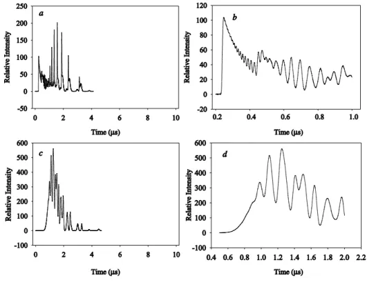
sweep rate was 0.684 kG/s, with the maximum magnetic field of 6.84 kG generated at 10 s sweep duration. Figure 1 shows typical experimental exchange resonance spectra obtained presently.
Figure 1a demonstrates the complete SA resonance spectrum for the Co (hCo = 7.6 nm), SiO2 (hd
= 7.9 nm), Fe (hFe = 7.9 nm) system, recorded within the total sweep range of 0 to 10 s, while
Figure 1b shows only the lower-field part of the same spectrum recorded at shorter sweep times. Figure 1c demonstrates the complete SA resonance spectrum for the ZnO (hZnO = 7.4 nm), SiO2
(hd = 7.6 nm), CuO (hCuO = 7.7 nm) system, recorded within the total sweep range of 0 to 10 s,
while Figure 1d shows only the lower-field part of the same spectrum recorded at shorter sweep times. Detailed analysis suggests that the spectra may be represented by a superposition of several independent spectral components, shown in Figure 2 and 3 respectively for the Co (hCo =
7.6 nm), SiO2 (hd = 7.9 nm), Fe (hFe = 7.9 nm) and ZnO (hZnO = 7.4 nm), SiO2 (hd = 7.6 nm),
CuO (hCuO = 7.7 nm) systems. These spectral components were extracted as described below.
Note that the experimental spectra contain discrete lines, some of these containing several superimposed individual contributions. Such composite lines were fitted by a sum of 2 or 3 Lorentz components:
3 , 2 , 1 2 , 1 ; 1 2 or i t B A t I i i i (3)where Ai, Bi, i are fitting parameters, while simple lines were represented by a single Lorenz
component (3) each. The entire set of the fitting parameters Ai, Bi and i was analyzed to
manually identify sequences of interrelated peaks, which resulted in 4 complete spectral sequences identified. The results are presented in Figures 2 and 3, with the line shapes always described by the function (3).
The structure of the spectral components shown in Fig. 2a-e in different from those of Figures 2d,f and will be discussed later. The structure of the spectral components shown in Figures 3a-c has the same nature as that of the components shown in Figures 2d,f and will be also discussed later. For now, we shall only note that we number the spectral lines in each of the components starting from the line located in the highest fields (later in the sweep) and continuing to those appearing in lower fields (earlier in the sweep). We interpret these line numbers MS as
projections of the total system spin on the external field direction [10-12]. Note also that the spectral components of Figure 2a-e may be assigned to the low-spin states (the exchange interaction is stronger than the spin-spin interaction), while the spectral components of Figures 2d,f and 3a-c may be assigned to high-spin states (the exchange interaction is weaker than the spin-spin interaction) [10-12].
We also found that the linewidths in the SA resonance spectra are significantly dependent of the nanolayer thickness. As an illustration, Figures 4, 5 and 6, show plots of the linewidth for the line number 3 in the spectral components of different samples in function of the thickness of the respective Co, ZnO and CuO layers.
The plots of Figures 4,5 and 6 may be fitted with good accuracy by the function
h hS e t t 2 1 0 (4)
used earlier [14], where t0 and h are empirical parameters, with the respective values
presented in Table 1. In Figures 4, 5 and 6, the plots marked by (a) – (e) correspond to the individual spectral components presented in Figures 2 and 3.
The comparison of the exchange resonance spectra obtained in the present study with those reported earlier for the ferromagnetic – dielectric – metal (FDM) three-layer sandwich device shows significant differences: the earlier recorded FDM spectra [10-14] have a regular peak structure – (a) the peak with the maximum intensity is located in the lowest field (the smallest time); (b) the peak intensity decreases with the magnetic field strength; (c) the gaps between the
peak maxima increase with the magnetic field strength; (d) the exchange resonance spectra can be described by a single spectral component. However, the presently recorded spectra are more complex, and will be interpreted using the theoretical models developed for such devices.
A detailed theory of the electronic gas and magnon waves in metals has been developed earlier, and presented elsewhere [15-17]; however, no detailed treatment had been proposed for the nanosandwich systems. Therefore, presently we shall limit our interpretation of the experimental data to the previously proposed empirical model [10-12]. We will also discuss the mechanisms explaining the results shown in Figures 4 – 6.
Note that the SA resonance effects disappear with the increased thickness of the Co, ZnO or CuO layers, becoming unobservable at thicknesses exceeding 1 m. Therefore, we conclude that such quantum effects are only observable in nanostructured systems.
Models and Discussion
a) Qualitative Interpretation of the Spectra
The observed effects have been explained qualitatively earlier [12]. Namely, a metal or a semiconductor nanolayer may be described as a 3D system, with a low-density discrete series of electronic states quantized in the z direction normal to the layer, and a high-density quasicontinuum of states quantized in the xy plane (of the layer). We assume that the states located in different isolated nanolayers interact by the exchange mechanism. Note that interactions between the quasicontinuum spectra of different nanolayers are irrelevant for our present purposes, resulting in classical magnetic momentum transport between nanolayers in presence of an external magnetic field. However, the interactions between the discrete spectra of different nanolayers may generate spin anticrossing effects in external magnetic fields, due to differing electron g-factors in the two interacting layers. Noting that the energies of the Fermi levels are also different in different nanolayers, we should expect strongly nonequilibrium populations in pairs of spin-polarized states coupled by the exchange interaction. The changes in the electron populations resulting from the equilibration will be observable via spin anticrossing effects, generated by the resonant transport of the spin polarization between different nanolayers.
Next, we shall briefly outline the earlier developed phenomenological theory describing the spin anticrossing spectra [10-12].
Co/Fe and ZnO/CuO sandwich systems
b) The phenomenological model
A detailed analysis of the phenomenological model has been presented earlier for the three-nanolayer systems [10-12]. The exchange resonance spin-anticrossing spectra shown in Figure 1 were considered in the framework of two coupled spin states. In the presently discussed structures, the second state is located in either the Fe or CuO nano-layer, each in direct contact with its respective SiO2 layer. The calculated values of the model parameters are presented in
Table 2, including 0 (cm-1), the zero-field energy gap between the coupled spin-states; f, the
relative weight of each of the components of Figure 2 and 3 in the original spectrum of Figure 1;
12
g
, the g-factor difference between the Co and Fe or ZnO and CuO layers; V12 , the matrix
element of the exchange interaction coupling the spin-states of interest; and 1 and 2, the widths of the coupled spin-states, dependent on the spin-lattice relaxation rates. Note that typical spin-lattice relaxation times are in the range of 0.1 – 1.0 s [18]. This two-coupled-spin-states model corresponds to a single exchange-interaction anticrossing peak with the selection rules SS1
= SS2 = S; MS = 0.
Table 2 shows that the g-factor differences between the Co and Fe and the ZnO and CuO layers are ca. 1.470 and 1.738, respectively. Note that that the g-factor values for the respective bulk materials are close to 2, therefore their respective differences as evaluated between bulk materials should be very small. However, we already noted [10-12] that significant deviations from the bulk g-factor values are possible in nanostructures, qualitatively explaining the results obtained. This conclusion is supported by the ab initio analysis of the nanolayer sandwich devices presented below.
c) Ab initio analysis
To carry out the ab initio analysis of the spectra obtained for the Co/Fe and ZnO/CuO three-nanolayer systems we used the earlier developed approaches [12-14]. The exchange interaction and the SO momentum coupling are the quantum phenomena directly responsible for the magnetic properties. Thus, the magnetocrystalline anisotropy can be explained using simple quantum statistical models, known as the Callen-Callen or Akulov law, as well as the T3/2 temperature dependence of the magnetization deviation from its 0K value (the Bloch law). However, the analytical models are unable to treat complex systems, therefore, numerical calculations are required. The full-Hamiltonian eigenvalue problem may only be solved in a few special cases, therefore, extra approximations are needed. Numerical analysis of a three-layer sandwich system may be performed using the coupled-cluster theory (CCT) with the magnetic phenomena included. Other approximations may also be used in the analysis of the system considered.
Presently we used the CCT and the local electron density approximation (LEDA), LEDA(GGA)+U and local spin density approximations (LSDA), adding the spin-orbit coupling to the functional in order to calculate the magnetic properties of the nanolayers. Note that LEDA and LEDA(GGA)+U approximations produce very similar results. Therefore, we carried out all of the calculations usung the LEDA approximation. The effective system Hamiltonian included only the magnetic-moment degrees of freedom in each of the nanolayers, and boundary conditions at the layer interfaces. Thus, we used the Hamiltonian in each of the nanolayers in the form [19-22]:
i z X i B X i j i z X j z X i X ij i z X i X i j i X j X i X ij X H m g m m d m d m m J H , 0 , , , 2 , 2 , 0 , ˆ ˆ (5)
where X = Co, SiO2, Fe, ZnO, or CuO layer, diX,0 is the single-ion anisotropy, dijX,2 is the
ion-pair anisotropy and Jˆij X is the effective exchange interaction parameter. Here mi X are sublattice elementary cell total spin-orbital angular momenta of the i-th electron, H is the
external magnetic field strength, and giX,0 is the electron g-factor determined below. Ideally,
the input data should include the crystal structure of the Si crystal (the substrate surface), and then the lattice structure of the Co nanolayer deposited on the Si substrate, that of the SiO2
nanolayer deposited on Co nanolayer, and those of the Fe nanolayer deposited on the SiO2
nanolayer for the first system, and the structure of the ZnO nanolayer deposited on the Si substrate, that of the SiO2 nanolayer deposited on Co nanolayer, and that of the CuO nanolayer
deposited on the SiO2 nanolayer, for the second system [23-28]. To simplify the calculations, we
considered the Co/vacuum/Fe and ZnO/vacuum/CuO structures, neglecting the effects of the substrate and the dielectric. The boundary conditions at the layer interfaces were set to minimize the system energy. Note that in the last step of the calculations, the elementary cell parameters were fixed. This approximation produced interface “stress” of ca. 0.1 – 0.3 eV, decreasing exponentially away from the interface. The average magnetic moments of ZnO and CuO are zero in bulk crystals but not in nanolayers, due to strong coupling between the ground state and the excited states with nonzero multiplicity.
d) Computational Methods
We used two independent ab initio approaches, as outlined below.
The first approach used commercial Gaussian – 2000 software package to calculate the wavefunctions. CCT, LEDA and LSDA methods were used with the 6-31G(d) basis set. The total number of atoms (216) in the 3D model of the sandwich structure was distributed between the Co layer (663 atoms) and the Fe layer (663 atoms), or the ZnO layer (663 atoms), and the CuO layer (663 atoms). The SiO2 layer was represented by a structureless vacuum
space with the thickness of
2
SiO d
d h
n SiO2 molecule diameters, where hd is the real thickness of
the dielectric nanolayer,
2
SiO
d being the average diameter of the SiO2 molecule. We also analyzed
a pseudo-1D model containing 108 molecules/atoms located as shown in Figure 7, with all of the chemical species represented by spheres with the respective average diameter: the 36 Co atoms that are in contact with each other and separated by an empty space from the 36 Fe atoms, which also are in contact with each other, etc. The number of atoms in the pseudo-1D model approximately corresponds to the double of the layer thickness divided by the respective atom
diameter, while the empty space width was chosen to produce the correct 2 SiO d d h n , with 2 SiO d being the SiO2 molecule diameter. Note that all of the calculations discussed above were
additionally repeated using the ROCK CLUSTER software package [29].
The results of the first step were used as input data for our home-made Fortran code that calculates the magnetic moment in function of the external magnetic field strength using the Hamiltonian (5), where the giX,0 values were calculated in the j-j coupling scheme as follows
[18,30]:
2
, 2 , 2 , 0 , , 2 , 2 , 2 , 0 , , 2 , 0 , , 2 1 X s i X l i X j i X s i X s i X l i X j i X l i X j i X j i s l j g s l j g j g (6)Here, gi,Xj,0 is the g-factor operator, gi,Xl,0 the orbital angular momentum g-factor, gi,Xs,0 is the
spin angular momentum g-factor, ji ,Xj is the total angular momentum,
X l i
l, is the orbital angular
momentum, and finally si ,Xs is the spin angular momentum, all of the i-th electron in the
nanolayer X.
The discussed approach gives the magnetic field strength dependences of the magnetic moment averaged over the output surface for the Co/vacuum/Fe and ZnO/vacuum/CuO three-nanolayer sandwich devices, producing a set of resonances in the same range of the magnetic field values as the experimental exchange resonance spectra. Our home-made FORTRAN code was used in the numerical analysis of both Equations (5) and (6).
The analysis started with the sets of eigenvalues
0 kE and eigenvectors
0 k obtained using the Gaussian-2000 or the ROCK CLUSTER software, used to calculate the average
X i z X i B X i m H g H V , , 0 ,
j i z X j z X i X ij i z X i X i j i X j X i X ij X m m d m d m m J Hˆ ˆ ,0 , 2 ,2 , , (7)These calculations were repeated for different values of the magnetic field strength, testing the
derivative
dH H V d
in order to find the extremum values Hext of V
H . The magnetic momentvalues corresponding to these extrema were calculated using
ext ext ext H H V H The results are shown in Table 3, where the positions of the resonances and the values of the output magnetic moments (proportional to the line intensity) are listed for both devices of interest and for both 3D- and pseudo-1D models. We see that the calculated peaks are in the same range as the experimentally observed anticrossing resonances, although no quantitative agreement could be achieved. Note that 0.684 kG/s sweep rate should be used to transform the sweep time scale into the magnetic field scale.
Note that we are considering quantum phenomena due to spin-state anticrossing effects induced by the exchange interaction between different layers. This interaction only exists when the total spin angular momentum and its projection on the magnetic field direction are the same for the two coupled states. The data of the Table 3 are also shown in Figure 8.
We also applied the second theoretical approach that was developed earlier [10-12] and uses the first-principles pseudopotential method within the spin density functional theory. The ultrasoft atomic pseudopotentials [31] and the generalized gradient approximation (GGA) [31] for the exchange and correlation potentials were used within the Quantum-ESPRESSO package [32]. We analyzed the same 4-layer structure, where the Si substrate was neglected. Namely, a -centered 669 k mesh was used to sample the irreducible Brilouin zone in the Monkhorst-Pack
scheme [33]. To improve the analysis accuracy so that neighboring exchange anticrossing peaks become resolved, the Methfessel-Paxton technique was adopted with a smearing width of 0.001 Ry [34,35]. The smearing procedure was used because of the Co and Fe nanolayers present in the first device. Convergence better than 510-6 eV was achieved for the total energy. We used published bulk crystal-lattice parameters for Co, Fe, ZnO and CuO [24-28]. The average value of the magnetic moment was calculated for the non-relaxed system at T = 77 K, assuming that the Fermi-state population distribution in the zero field is conserved in presence of a finite magnetic field. Note that in comparison with the first approach, the second approach reproduces the same resonance peaks shown in Figure 8, albeit with a different intensity distribution. Typical SA spectra obtained by the second approach are shown in Figure 9.
The calculations presented in Figures 8 and 9 only produce the line intensity and position; the line widths were not calculated, as the spin relaxation was disregarded. However, the spectrum of Figures 8 and 9 has finite line widths, introduced as phenomenological parameters for better presentation. The calculated spectrum qualitatively reproduces the positions of the experimental lines. Once more we note the insufficient accuracy of the present numerical approach, excluding quantitative agreement with the experimental spectra.
The magnetic properties of different materials have been extensively studied earlier using the ab initio approach [31-35]. However, there are no publications discussing systems similar to those presently studied. In the present study, we used the previously proposed numerical methods [10-12] that we modified by adding the Zeeman interaction term. The state anticrossing effect was created by the exchange interaction between the Zeeman substates with coincident MS and S
values, where S is the total system spin angular momentum and MS its projection on the field
direction. Note that the spectra calculated in both the 3D and 1D models reproduce the experimental spectrum with a similar level of accuracy. Recalling that the experimental device used the needle tip 50 m in diameter, a better model should consider interactions between three disks 50 m in diameter and 8 nm thick. Presently, it is not possible to do ab initio calculations for such a large system. An alternative approach that we shall pursue involves representing the nanolayers as continuous media, with the electrons moving within certain potentials. We also
disregarded hyperfine interactions, which result in the quantization of the total angular momentum F = S + L + I, as the accuracy of our experimental and calculation methods was insufficient for the hyperfine structure to be resolved. This issue will be addressed in a future study.
Let us now discuss the data shown in Figures 4 to 6. The data were fitted using an empirical relationship (4), with the values of the parameters listed in Table 1. The line width in the SA spectrum is determined by the relaxation of the spin states of interest, the zero-field energy gap between the interacting spin states, the difference of the g factors of the coupled spin states and the projection of the total spin angular momentum on the field direction [10-12]. In the frameworks of the developed theory, we can not calculate the relaxation properties of the spin states of interest; however, we can analyze the dependence of the zero-field energy gap between the interacting spin states as well as the difference of the g factors of the coupled spin states. Both these dependences were calculated using the second approach (see above) applied to the Pseudo-1D model (see above). We analyzed the respective dependences in function of the number of the Co “atoms” in the model shown schematically in Figure 7, plotted in relative units as a function of the Co atom effective radius, as adding one atom to the chain, its length increases by one atomic radius. The respective plots are shown in Figures 10a,b.
As it it follows from the Figure 10 that the E value decreases slower than g. Thus, the g-factor contribution that increases the line width is more significant than that of the respective energy gap that decreases the line width. Using the phenomenological model developed earlier [10-12] and the data presented in Figure 10, we calculated the dependence of the linewidth on the Co nanolayer thickness for the line number 3 in the SA spectrum, with the results shown in Figure 10b. Note that the latter dependence was calculated for fixed values of the relaxation parameters describing the relaxation properties of the coupled spin states. These results qualitatively describe the experimental data of the Figures 4 to 6. Note also that the SA resonance spectrum disappears if the active material thickness exceeds 1 m.
Conclusions
The proposed novel spintronic device operates on magnetic moments of the electronic spin states in different nanolayers. Our phenomenological model assumes that the spin state gets transferred from one layer to another, detached from the respective electrons, which can't be transported through the relatively thick dielectric layer. The strength of the interaction inducing spin-polarized state transport is controlled by the thickness of the dielectric layer. We predict that oscillations (the observed exchange-resonance peaks) of the magnetic field strength may be created in the device, provided a sufficiently fast external magnetic field pulse is applied. The spin-polarized spectrum generated by the device consists of S discrete bands, where S is the total spin angular momentum in one of the conductive/semiconductive layers coupled by the exchange interaction to another layer. The proposed model was partially verified by the experiments [10-12]. Presently, we tested new devices with Co/Fe and ZnO/CuO structures, using Co and ZnO as the first of the two conductive/semiconductive nanolayers, respectively. The output signals of the Co/Fe and ZnO/CuO devices are different from those of the previously studied devices [10-12]. Our phenomenological model was used to fit the experimental spectra, achieving good agreement with the experimental results. The fitting procedure produced estimates of the model parameters; their physical interpretation and possible mechanisms involved have been discussed earlier [10-12]. Ab initio analysis of the three-nanolayer devices demonstrated that magnetic field dependence of the output signal averaged over the surface has resonant structure. Presently, such methods are unable to provide the accuracy needed to reproduce the detailed structure of the experimental spectrum, producing only a qualitative agreement. We expect that increasing of number of atoms in modeling system will increase accuracy and provide better agreement between experimental and ab initio theoretical spectra.
Acknowledgement: V.M. is very grateful for the financial support from the DoE Grant
References
[1] C. Kittel, Introduction to Solid State Physics (WSE, Wiley, New York, 1973). [2] R.A. Serota, arXiv:cond-mat/0007297v1, 18 Jul 2000.
[3] V. A. Koziy and M. A. Skvortsov, arXiv:1106.3863v1, 20 Jun 2011. [4] E. Hofstetter, M. Schreiber, arXiv:cond-mat/9408040v1, 12 Aug 1994.. [5] K. R. Barqawi, Z. Murtaza, T. J. Meyer, J. Phys. Chem., 95, 47 (1991). [6] X-F.F. Wang, Z. Wang, G. Kotliar, Phys. Rev. Lett., 68, 2504 (1992)
[7] W. Hubner and K. H. Bennemann, arXiv:cond-mat/9508120v1, 25Aug1995.
[8] R. E. George, W. Witzel, H. Riemann, N.V. Abrosimov, N. Notzel, M. L.W. Thewalt, J. J. L. Morton, Phys. Rev. Lett. 105, 067601 (2010)
[9] V. P. Zhukov, E. V. Chulkov, P. M. Echenique,, Phys. Stat. Sol., (A) 205, 1296 (2008).
[10] V.I. Makarov, S. A. Kochubei, I. Khmelinskii, J Appl. Phys. 110 (2011) 063717. [11] V.I. Makarov, Khmelinskii I., Material Research Bulletin., 50, 2014, 514-523. [12] V. I. Makarov, I.V. Khmelinskii. J. Appl. Phys., 2013, 113, 084304 (+9 pp.); [13] V. I. Makarov, I. Khmelinskii, arXiv: 1405.5243, 13 May 2014,
http://arxiv.org/ftp/arxiv/papers/1405/1405.5243.pdf, visited: September 2014. [14] V. I. Makarov, I. Khmelinskii, arXiv: 1405.4889, 13 May 2014,
http://arxiv.org/ftp/arxiv/papers/1405/1405.4889.pdf, visited: September 2014.
[15] R.P. Feynman, “Statistical Mechanics.” California Institute of Technology, W.A. Benjamin Inc., Advanced Book Program Reading, Massachusets 1972.
[16] E.M. Lifshic, L.P. Pitaevskii, Physical Kinetics, Butterworth Heinemann, Oxford, Boston, Johannesburg, 9th Edition, 1997.
[17] C. Kittel, “Quantum Theory of Solids” Department of Physics, University of Berkley, California, John Wiley & Sons Inc., New York – London, p.p. 64 – 92, 1963.
[18] A. Carrington, A.D. McLachlan, Introduction to Magnetic Resonance., Harper&Row Publisher, 1967.
[19] Dan Li, Yousong Gu, Zuoren Nie, Bo Wang, Hui Yan, J. Mater. Sci. Technology., 22, 2006, 833.
[20] M.F. Islam, C.M. Canali, Phys. Rev., 85, 2012, 155306.
[21] X. Qian, F. Wagner, M. Peterson, W. Hubner, J. Magnetism & Magnetic Materials 213, 2000, 12.
[22] Ya. Kouji; S. Kunio, O. Toru. Metallurgical and Materials Transactions B 42: (2010) 37. [23] R. Hull,.Properties of crystalline silicon.,. p. 421 (1999). ISBN 978-0-85296-933-5
[24] M. Riordan, The Silicon Dioxide Solution: How physicist Jean Hoerni built the bridge from the transistor to the integrated circuit., IEEE Spectrum, (2007).
[25] R. Doering, Yo. Nishi, Handbook of Semiconductor Manufacturing Technology. CRC Press. ISBN 1-57444-675-4 (2007)..
[27] A.B.D. Nandiyanto, S.G. Kim, E. Iskandar, K. Okuyama, Microporous and Mesoporous Materials 120 (3): 447 (2009)..
[28] H. W. Richardson "Copper Compounds in Ullmann's Encyclopedia of Industrial Chemistry 2002, Wiley-VCH, Weinheim. doi:10.1002/14356007.a07_567
[29] E. Wiberg, A.F. Holleman, Inorganic Chemistry. Elsevier. ISBN 0-12-352651-5 (2001). [30] A. Gonzalez-Garcia, W. Lopez-Perez, R. Gonzalez-Hernandez, Computational Material Science, 55 (2012) 171.
[31] M. Černý, J. Pokluda, M. Šob, M. Friák, P. Šandera, Phys. Rev. B 67 (2003) 035116.
[32] J Wang, J-M Albina, Y Umeno, Journal of Physics: Condensed Matter, 24 (2012) 245501; J Wang et al, J. Phys.: Condens. Matter 24 (2012) 245501
[33] G. Lopez Laurrabaqio, M. Perez Alvarez, J.M. Montejano-Carrizales, F. Aguilera-Grania, J.L. Moran-Lopez, Revista Mexicana de Fisica, 52 (2006), 329.
[34] M. Werwinski, A. Szajek, P. Lesniak, W.L. Malinowski, M. Stasiak, Proceeding of the European Conference Physics of Magnetism, 2011 (PM11) Poznan, June 27 – July 1, 2011. [35] M. Ekholm, A. Abrikosov, Phys. Rev., B 84 (2011), 104423.
Figure 1. The experimental spin-anticrossing resonance spectra (a, b) Co (7.6 nm) – SiO2 (7.9
nm) – Fe (7.9 nm) sandwich structure; (c, d) ZnO (7.4 nm) – SiO2 (7.6 nm) – CuO (7.7 nm)
sandwich structure, all recorded at 77 K (LN2).
Figure 2. The spectral components extracted from the experimental spectrum of Fig. 1 (a).
Figure 3. The spectral components extracted from the experimental spectrum of Fig. 1 (c).
Figure 4. The Co layer thickness dependences of the linewidths in the Co – SiO2 (7.9 nm) – Fe
(7.9 nm) three-layer sandwich structure; (a) to (f) refer to the respective spectral components of Fig. 2.
Figure 5. The ZnO layer thickness dependences of the linewidths in the ZnO – SiO2 (7.6 nm) –
CuO (7.7 nm) three-layer sandwich structure; (a) to (c) refer to the respective spectral components of Fig. 3.
Figure 6. The CuO layer thickness dependences of the linewidths in the ZnO (7.4 nm) – SiO2
(7.6 nm) – CuO three-layer sandwich structure; (a) to (c) refer to the respective spectral components of Fig. 3.
Figure 7. The atomic chain used in the pseudo-1D model.
Figure 8. The ab initio spectra obtained using the first approach for the 3D- and Pseudo-1D models for the Co/vacuum/Fe and ZnO/vacuum/CuO systems.
Figure 9. The ab initio spectra obtained using the second approach for the 3D- model for the Co/vacuum/Fe and ZnO/vacuum/CuO systems.
Figure 10. (a) the ab initio Co layer thickness dependences of g and E parameters of the phenomenological model [10-12] for the Co/vacuum/Fe system using the second approach for the pseudo-1D model; (b) the dependence of the linewidth (line number three) on the Co layer thickness calculated using the phenomenological model.
Fig. 1
Fig. 3
Fig. 5
Fig. 6
Table 1. The values of the phenomenological parameters t0 and h for the components of the
exchange-resonance spin-anticrossing spectra of Fig. 2.
Figure 4 t0 (s) h (nm) (a) 21.9 5.1 (b) 19.7 5.9 (c) 23.9 6.3 (d) 9.2 4.1 (e) 20.3 4.7 (f) 7.1 3.2 Figure 5 t0 (s) h h (nm) (a) 11.6 4.7 (b) 12.3 3.3 (c) 10.6 4.9 Figure 6 t0 (s) h h (nm) (a) 13.1 3.1 (b) 14.2 4.2 (c) 12.7 6.5 TABLES
Table 2. Values of the phenomenological model parameters. S 0, cm -1 Relative contribution 12 g V12 , cm-1 1 , cm-1 2 , cm-1 Co – Fe (a) 21 0.0612 0.15 1.673 1.5110-4 1.0210-4 1.1110-4 (b) 35/2 0.0514 0.17 1.525 1.5810-4 1.1710-4 1.3210-4 (c) 19 0.0697 0.21 1.763 1.6210-4 1.3610-4 1.2110-4 (d) 25/2 0.0711 0.23 1.712 1.7310-4 1.1510-4 1.3210-4 (e) 17/2 0.0741 0.15 1.576 1.4710-4 1.2510-4 1.1210-4 (f) 16 0.0642 0.09 1.738 1.7810-4 1.1110-4 1.3510-4 ZnO – CuO (a) 13/2 0.0675 0.38 1.684 1.6310-4 1.2110-4 1.3310-4 (b) 21/2 0.0719 0.34 1.470 1.9110-4 1.1610-4 1.4210-4 (c) 15 0.0786 0.28 1.731 1.4510-4 1.1010-4 1.2610-4
Table 3. The locations and the line intensities of the calculated resonance peaks for the Co/vacuum/Fe and ZnO/vacuum/CuO structures for both 3D- and pseudo-1D models. Co/vacuum/Fe 2D Model Position, kG Magnetic moment, B 2D Model Position, kG Magnetic moment, B P-1D Model Position, kG Magnetic moment, B P-1D Model Position, kG Magnetic moment, B 6.72 1.11 3.12 1.42 6.57 0.81 3.02 1.47 6.61 1.02 2.69 1.65 6.54 0.72 2.51 1.59 6.53 0.95 2.24 1.98 6.52 0.82 2.22 1.91 6.51 0.92 1.93 2.29 6.50 0.79 1.89 2.31 6.32 0.84 1.72 2.57 6.31 0.84 1.65 2.53 6.09 0.92 0.89 4.97 6.15 0.98 0.97 4.87 5.71 1.21 0.69 6.42 5.73 1.01 0.61 6.41 5.33 1.10 0.41 10.80 5.28 1.08 0.45 10.79 5.01 1.15 0.40 11.07 4.93 1.05 0.41 11.11 4.53 1.13 0.39 11.35 4.38 1.13 0.33 11.39 4.02 1.20 0,36 11.48 4.01 1.21 0,31 11.53 ZnO/vacuum/CuO 2D Model Position, kG Magnetic moment, B 2D Model Position, kG Magnetic moment, B P-1D Model Position, kG Magnetic moment, B P-1D Model Position, kG Magnetic moment, B 6.23 0.82 3.11 1.22 6.47 0.94 3.01 1.27 5.75 0.73 2.57 1.45 5.79 0.98 2.47 1.67 5.25 0.86 2.21 1.79 5.31 0.81 2.31 1.85 4.68 0.84 1.82 2.37 4.61 0.93 1.89 2.39 4.33 0.91 1.52 2.58 4.39 0.99 1.57 2.78 4.06 1.09 0.77 4.90 4.14 1.16 0.67 4.93 3.27 1.07 0.52 6.48 3.59 1.23 0.59 6.57